Synthesis of Vegetation Indices Using Genetic Programming for Soil Erosion Estimation

Abstract

Vegetation Indices (VIs) represent a useful method for extracting vegetation information from satellite images. Erosion models like the Revised Universal Soil Loss Equation (RUSLE), employ VIs as an input to determine the RUSLE soil Cover factor (C). From the standpoint of soil conservation planning, the C factor is one of the most important RUSLE parameters because it measures the combined effect of all interrelated cover and management variables. Despite its importance, the results are generally incomplete because most indices recognize healthy or green vegetation, but not senescent, dry or dead vegetation, which can also be an important contributor to C. The aim of this research is to propose a novel approach for calculating new VIs that are better correlated with C, using field and satellite information. The approach followed by this research is to state the generation of new VIs in terms of a computer optimization problem and then applying a machine learning technique, named Genetic Programming (GP), which builds new indices by iteratively recombining a set of numerical operators and spectral channels until the best composite operator is found. Experimental results illustrate the efficiency and reliability of this approach to estimate the C factor and the erosion rates for two watersheds in Baja California, Mexico, and Zaragoza, Spain. The synthetic indices calculated using this methodology produce better approximation to the C factor from field data, when compared with state-of-the-art indices, like NDVI and EVI.

1. Introduction

Soil erosion is a natural process that detaches and transports soil material through the action of an erosive agent like water, wind, gravity, or anthropogenic perturbations [1]. In most arid areas, irregular and intense precipitation is the main cause of erosion. This phenomenon is aggravated in terrains that have either pronounced slopes, soft or non-consolidated lithology, or sparse vegetation. An important factor that increases erosion is inappropriate land management, mostly by overexploitation of the soil or deficiently-planned engineering projects [2]. Soil erosion by water is the most important land degradation problem at a global scale, since it produces a strong environment impact and high economic cost due to its effects on agricultural production, civil infrastructure, and water quality [3]. Therefore, in order to improve soil conservation measures, it is necessary to monitor areas that are vulnerable to the effects of erosion.

Studies about soil conservation and its main contributing factors have produced predictive erosion models. Some of them are empirical (based on the evaluation of statistical-based coefficients that were derived from field observations in several areas of the world) like the Revised Universal Soil Loss Equation (RUSLE), and some of them are physical (determine certain parameters that represent the mechanisms that control erosion) like the Water Erosion Prediction Project (WEPP) [4,5,6,7]. These models allow predicting soil erosion and its impact in small regions. However, it is difficult to estimate erosion precisely at a large scale due to the significant number of parameters involved and the complexity of determining each one of them. Therefore, there is a need to develop new methods to determine erosion parameters and their effects on soil loss.

The USLE model [8] included the following parameters: specific soil type, rain patterns, and the region’s topographic properties. The revision to the USLE model (RUSLE) [7] improved measurement methods for the original parameters and eased the use of computers for faster data processing, which has caused this model to be frequently employed to predict annual average soil loss. The equation for the RUSLE model includes six factors that numerically express the physical characteristics of erosion:

$$A=R\times C\times S\times L\times K\times P,$$

(1)

R is the rainfall erosivity, which is the erosive energy produced by precipitation and drainage; this parameter is measured as the product of the storm’s total energy, E, by the maximum intensity in a 30-min period. Crepresents the cover factor. It measures the combined effect of all interrelated cover and management variables. In the case of forest basins, such as those presented in this work, the C factor is dominated by vegetative cover. According to the RUSLE model [7], $C=1$ represents bare recently-plowed soil, $C=0.45$ is used for unaltered bare soil, and $C=0$ is employed for soil that is completely covered. S and L determine the topographic conditions of the area, where L is the slope’s length factor, which is scaled to a standard length of 22.13 m; and S is the slope’s steepness, which is normalized to a standard $5.1{}^{\circ }$. K is the soil erodibility and is based on the soils’s texture and structure. P is the support practice factor and is used to represent soil management and conservation activities, where a value of $P=1$ represents a zone with no soil management practices.

From the ecological point of view, vegetation cover is defined as the different coverings that protect soil from the direct action of precipitation. The vegetation cover factor can be easily measured at a local scale in agricultural fields because it is generally homogeneous and the dimensions of the area are well defined. However, it is difficult to quantify this factor at a regional scale because it requires a large amount of time to take individual samples. Nevertheless, recent works have proven that erosion can be estimated at the global scale with an innovative methodology for the C-factor [9]. This article is one more step in that trend by proposing a new methodology that allows one to better determine the vegetation cover factor, C, at a regional scale.

Current technology has made it possible to obtain satellite images easily and to develop computational tools to extract and process the information needed to calculate some biophysical properties at the Earth’s surface; for example, the Absorbed Photosynthetically Active Radiation (APAR), the net CO${}_2$ exchange in a local ecosystem ($NE{E}_{C{O}_2}$) [10], or the primary net production [11]. In particular, many methodologies have been developed to identify vegetation coverings, for example: spectral classification methods [12,13,14], fractional vegetation cover methods [15], and vegetation indices [16,17,18,19,20,21,22]. However, most of these methods have been designed to focus mainly on green vegetation, and not on dry or dead vegetation, which are required by erosion models to assess the vegetation cover factor [4].

This paper proposes a novel methodology based on a machine learning technique named Genetic Programming (GP) to obtain accurate estimation of one of the main factors for the RUSLE model: the vegetation Cover (C) factor. In this methodology, the problem of calculating the cover factor is stated as an optimization problem, where the objective is to find the vegetation index that shows a better correlation with the C factor from field data. In this way, the GP-based algorithm synthesizes new vegetation indices by means of an iterative combination of arithmetic operators and spectral bands from satellite images. This paper is organized as follows: Section 2 presents a literature review of machine learning-based methodologies for estimation of the cover factor for soil erosion assessment. Section 3 describes the proposed methodology. Section 4 presents the results of the applied methodology in two semi-arid climate watersheds, and Section 5 presents the conclusions.

2. Related Work

In general, machine learning techniques allow one to analyze a set of data exhaustively and generate results that might not be evident to the eyes of an expert. Therefore, these techniques have been employed to derive new equations and mathematical models to represent complex systems and interactions [23,24,25]. The following is an analysis of previous research that has employed machine learning techniques to extract the C factor from satellite images. This paper classifies this research into three different approaches: The spectral classification approach consists of obtaining a thematic map by any classification method (maximum likelihood, ISODATA, K-means, object-oriented classification, etc.), and once this map has been obtained, a C factor value is assigned to the map’s regions that have similar surface coverage characteristics. The fractional vegetation cover approach is based on the assumption that the spectral signature of a pixel is the linear combination of the elements that the sensor records on the surface [26]. This technique is able to estimate the fractional abundance of ground vegetation and bare soil simultaneously in one pixel. Finally, the vegetation index approach applies arithmetic formulas to the spectral bands of a satellite image in order to enhance the signal representing the vegetation cover. Then, the obtained indices are correlated with the C factor using regression analysis (mainly linear regression).

An example of a spectral classification method was reported in [27], where a Land Transformation model (LTM) and the USLE model were employed to derive land cover dynamics and predict soil erosion. This study tried to identify and forecast future Land Cover (LC) using the LTM. The proposed LTM applies artificial neural networks algorithms for predicting LC, by considering pixel variations from the past and using spatial features. The researchers found that this approach is suitable for forecasting LC and predicting the variability of the C map, at the expense of recording several years of satellite images for the study area. A general limitation of spectral classification studies is that the thematic map usually defines homogeneous regions that lack the variability needed to measure the C factor precisely. Therefore, thematic maps are not an appropriate tool to reflect the natural spatial variability of the C factor.

A predictive RUSLE model and the fractional vegetation cover method were used to estimate the hillslope erosion hazard due to water erosion across New South Wales (NSW), Australia [28]. Values for the C factor were obtained from the emerging time-series fractional cover products derived from the Moderate Resolution Imaging Spectroradiometer (MODIS). Time-series C factor and hillslope erosion maps were produced for NSW on monthly and annual bases for a 13-year period using automated computer programs in a geographic information system. Although this study did not employ proper machine learning techniques, the estimated C factor values had better consistency in spatial and temporal contexts, compared with previous studies and field measurements in NSW.

Fractional vegetation cover methods have shown good performance in the classification at the subpixel level because they provide more variability to the C factor maps. However, the main weakness of these methods is the need to perform an efficient unmixing process in order to avoid misclassification; thereby, it is necessary to know a priori the components being measured within a pixel.

In the literature reviewed for this article, it was found that the only machine learning studies that have tried to use the synthesis of vegetation indices for the C factor are the works by Puente et al. [29] and Trabucchi et al. [30]. In [29], a first approximation to the synthesis of vegetation indices using Genetic Programming (GP) for the Todos Santos basin was reported with positive results; while [30] showed how synthesized vegetation indices are able to identify areas prone to erosion in the Rio Martin basin. Vegetation indices and specifically NDVI have been widely used in studies dealing with landslide [31], susceptibility to soil erosion [32,33], and gully erosion [34].

There are two main reasons for applying GP for synthesizing the C factor. The first one originates because traditional vegetation indices are designed to measure the state of green vegetation; however, erosion can be prevented even by dead and brown vegetation. This causes an imperfect correlation between the traditional indices and the C factor; therefore, GP could be used as an attempt to generate new indices that are more suitable for predicting the C factor. The second reason is that other machine learning techniques provide positive results, but do not show how these results were derived. GP is a technique that shows the combinations and operations that produced the resulting model [35].

This research proposes a new methodology based on GP with the objective of producing a precise estimate for the RUSLE’s vegetation cover factor. In this methodology, the estimation is treated as an optimization problem where the objective is to find the VIs with the strongest correlation to the C factor obtained from field samples. The GP algorithm is applied to find new vegetation indices based in the iterative combination of a set of numerical operations and spectral bands from satellite images. A standardized method that would allow automating the derivation of the C factor could be an important step towards improving the erosion estimation, as well as providing a significant reduction in costs, thus allowing regional- and global-scale application [1,4].

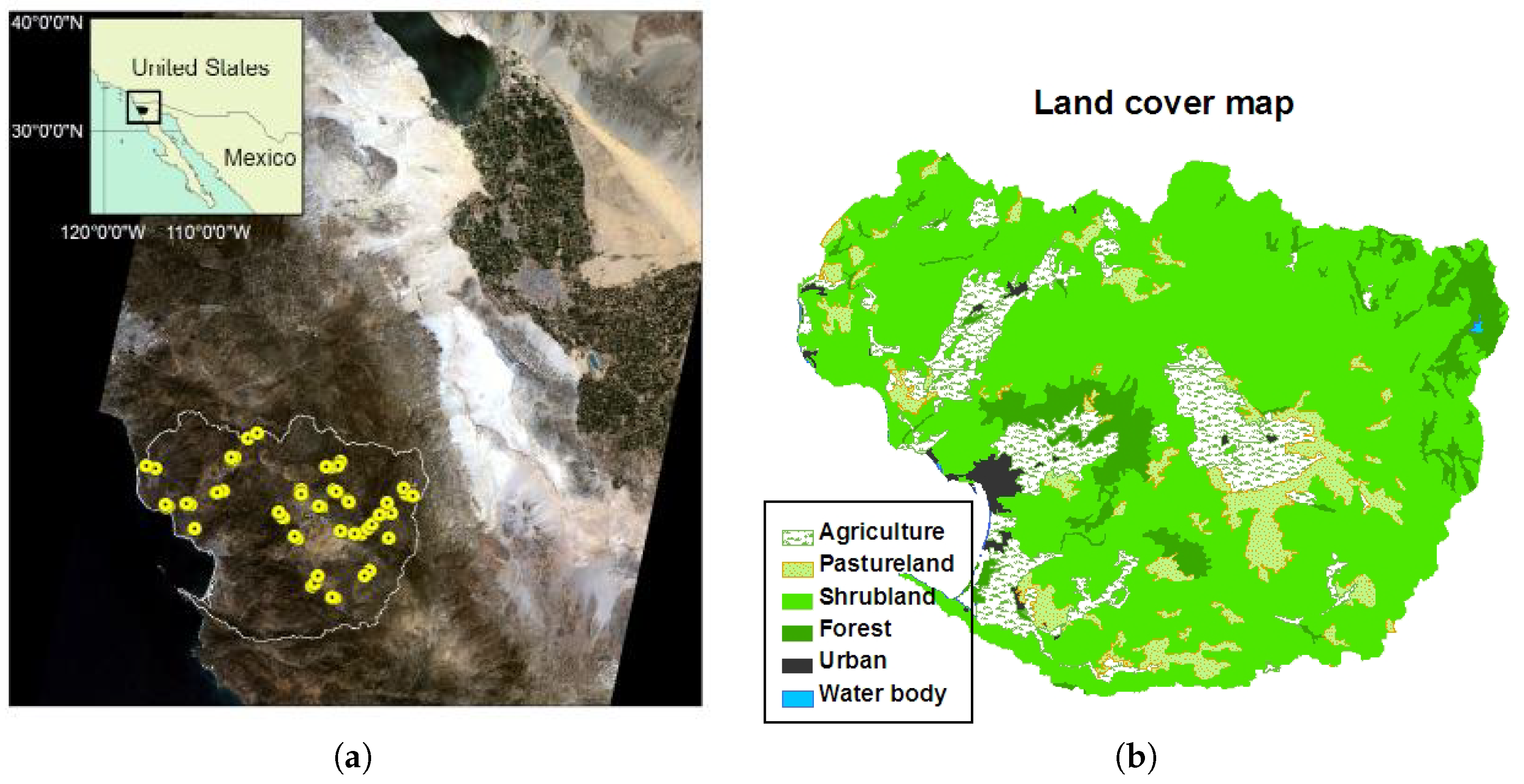
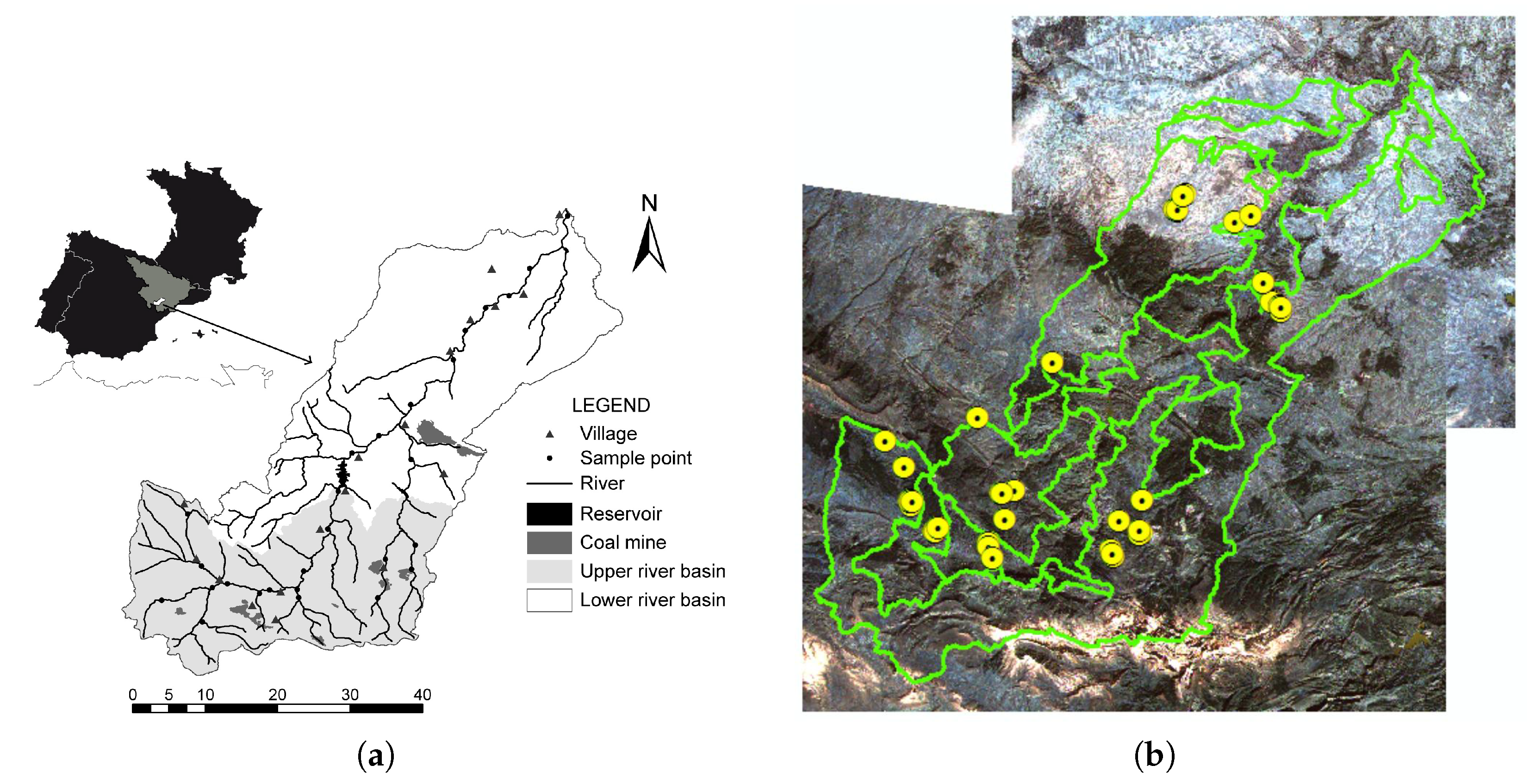
3. Study Area

This study was performed using two different watersheds or basins with semi-arid climate (BSh and BSk, according to the Köppen climate classification [36]): the Todos Santos watershed in Baja California, Mexico, and the Rio Martin watershed in Spain. Both areas were divided into two sections: one section provided samples for the training stage of the GP algorithm, while the other’s samples were employed for the validation stage.

The Todos Santos watershed (Figure 1) is located in the northwest part of the Baja California peninsula in Mexico [32]. It covers an area of 4900 km², and its elevation varies between 0 and 1876 m a.s.l. This watershed has two large alluvial valleys at 300 m a.s.l.: Guadalupe and Ojos Negros; and the city of Ensenada is located in a coastal plain at an average of 50 m a.s.l.

The climate is Mediterranean with mild wet winters and warm dry summers. The annual mean temperature is $16{}^{\circ }$C $\pm 6{}^{\circ }$C, and the mean annual rainfall is 315 mm; 85% of it falls in November and April [38]. As can be observed in Figure 1b, the native vegetation is mostly shrubs, which includes chaparral and coastal scrubs [37]. This type of vegetation covers 69% of the total area; agricultural land occupies 22% of the total area; while other covers, including permanent green woods and urban zones, occupy the remaining 9%. Areas that have slopes with less than $2^{\circ }$ are usually occupied by agricultural land and shrubs, while areas with steeper slopes are mostly covered by shrubs [32].

The Rio Martin watershed (Figure 2) is part of a larger watershed, the Ebro River, in southeastern Spain. It covers an area of 2111 km${}^2$, and its elevation varies between 143 and 1620 m above sea level. This watershed is divided into two pluvial zones: the high zone has 764 km${}^2$, while the low zone has 1347 km${}^2$. Each one has a dam, Escuriza and Cueva Foradada, respectively, which interrupts the water’s natural flow and establishes an environment that has been altered by human activity [30].

The climate is Mediterranean with dry summers and winters. The annual mean temperature varies between $13{}^{\circ }$C and $16{}^{\circ }$C, and the average annual rainfall is 360 mm; most of it falls in November and April. The natural vegetation has been heavily modified by human activity, although it is still characteristically Mediterranean. In the south, vegetation is dominated by low, dry weather-resistant bushes, which have replaced woods degraded by farming and fires for over 5000 years. Towards the north, bushes are substituted by oaks, thickets, and scrub. The highlands are 68% covered by native thickets and bushes, as well as pine woods that have been recently reforested. The lower watershed is mostly used for agricultural activities.

This paper describes how to calculate the vegetation cover factor C using satellite images’ data from both watersheds. The analysis for Todos Santos will be discussed in Section 5.3, while the one for Rio Martin has been already reported in [30], which used this information to propose restoration activities in this watershed.

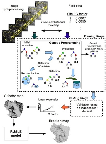
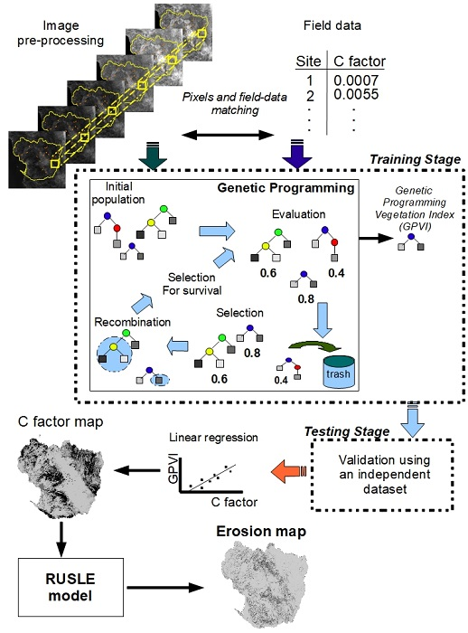
4. Methodology

Figure 3 shows a flowchart of the methodology followed in this paper. Its main objective is to develop an automated process to define a Vegetation Index (VI) that is strongly correlated with RUSLE’s C factor. This methodology may be divided into seven steps: (1) collecting field samples, (2) acquisition and correction of the satellite images, (3) associating satellite images with field data, (4) applying conventional VIs, (5) applying the GP algorithm, (6) the results’ evaluation, and (7) C factor map and erosion map generation. The following subsections explain each of these steps.

4.1. Collecting Field Samples

The procedure described in the RUSLE Manual [39,40] was employed to sample the field parameters that determine the C factor; namely, canopy cover, surface cover, surface roughness, prior land use, and soil moisture. This method was intended to be used in agricultural land with homogeneous covering conditions; not in semi-arid natural fields, which is the case for the watersheds in this study. However, in [41], the authors stated that for semi-arid watersheds with a low presence of arable lands, prior land use and soil moisture contribute little weight to the final C value. Hence, This paper decided to estimate the C factor by employing just three sub-factors that compose it [8]: superficial cover percentage, aerial vegetation cover, and residual underground factor. The superficial cover percentage may be obtained through the percentage and the height of aerial cover, while the residual underground factor can be calculated through the roughness and the underground biomass parameters.

Before the field data collection started, an analysis of both study areas was performed using satellite images and topographical maps, to define representative sampling zones. Each of these zones is called a sampling region, and they were selected to be areas of $100\times 100$ m with a high homogeneous distribution for the vegetation cover, altitude, and slope. The field data collection process for Todos Santos was performed between February and May 2007. In total, samples from 106 sites [41,42] were taken; while for Rio Martin, 40 sampling regions [30] were sampled in January and February 2009. The same procedure was employed for sampling both areas, the linear transect method [43,44]. In order to assign a single value to a complete transect, the average value of its 20 sampled points was used. The following parameters were determined using this method:

• Superficial cover percentage (g). This was visually determined from 10 cm around a dropped weight, otherwise known as the micro-plot. Each micro-plot was labeled with one of five different classifications according to the percentage of ground covered by vegetation or rocks: 0 = 0–1%, 1 = 1–25%, 2 = 25–50%, 3 = 50–75%, and 4 = 75–100%.
• Percentage (p) and height (h) of aerial vegetation cover. The percentage, p, is obtained using a similar method as for the superficial cover percentage: labeling a micro-plot according to the same five classifications. However, the center of the micro-plot is not defined by a dropped weight, but by the wire from which it hangs. The height, h, of the aerial cover for the sampling point is defined by the plant or its ramifications that are closest to the ground (without touching it) and touch the wire.
• Roughness (r) and underground biomass (b). Roughness, r, is evaluated according to the empirical method proposed by [41] and Tables 5-5 and 5-6 from the RUSLE manual [7]. Underground biomass, b, is inferred using the primary productivity method defined by [45]. For this study, b was assumed to be uniform.

Using these parameters, the C factor for each sampling point was defined using Equation (2). That equation was proposed by [41], which shows a good approximation to the values in Table 10 of the USLE manual [8] for semi-arid climates:

$$C=0.45(e^{[-0.012·b]})·(1-p·e^{[-0.328·h]})·e^{(-0.039·g·{[\frac{0.24}{r}]}^{0.08})}.$$

(2)

4.2. Satellite Image Acquisition and Correction

The images used to perform the field analysis came from the Landsat 5 satellite. Each image covers a square area, where each side measures approximately 185 km, and includes the seven frequency bands shown in

Table 1. Satellite frequency bands.

Band	Name	Wavelength
1	Blue light (B)	0.45–0.52 $\mathsf{\mu }$m
2	Green light (G)	0.53–0.60 $\mathsf{\mu }$m
3	Red light (R)	0.63–0.69 $\mathsf{\mu }$m
4	Near-Infrared (NIR)	0.76–0.90 $\mathsf{\mu }$m
5	Shortwave Infrared Channel 1 (SWIR1)	1.55–1.75 $\mathsf{\mu }$m
6	Thermal Infrared (TIR)	10.4–12.5 $\mathsf{\mu }$m
7	Shortwave Infrared Channel 2 (SWIR2)	2.08–2.35 $\mathsf{\mu }$m

. These cover the visible and infrared electromagnetic spectrums and have a resolution of $30\times 30$ m per pixel. Band 6, thermal infrared, is not considered relevant for this type of study [15,26,28,29,30,32]. Therefore, we decided not to use it.

The image taken when the Landsat 5 flies over the Todos Santos watershed is identified as “Path 39, Row 037” [46]. A section of the Rio Martin watershed is included in “Path 199, Row 031” and another in “Path 199, Row 032” [47]. It is necessary to correct these images to eliminate distortions, which modify the information. These distortions and the process employed to correct them are described below:

• Atmospheric correction corrects image distortions caused by humidity and other gases in the atmosphere. This research employed the Dark Pixel Correction (DPC) method [48]. Figure 4a,b shows the atmospheric correction for the Rio Martin watershed.
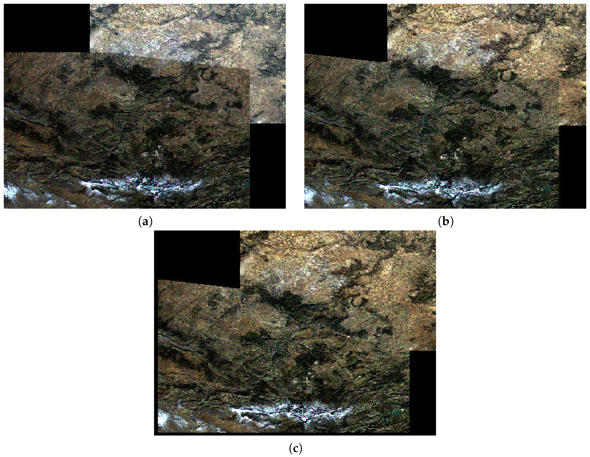
• Radiometric correction diminishes the effects of sensor miscalibration. It also corrects the distortions caused by the angle between the Sun and the satellite over the study area. In order to correct the images produced by the satellite, researchers employ the parameters and methodology published by NASA for instrument recalibration and pixel reflectance values [49]. Figure 4a shows two non-corrected images that were taken at different times; by applying the radiometric correction (Figure 4c), the pixel values are normalized, and the results are comparable.
• Geometric correction adjusts the satellite images to the geographic coordinate system. To perform this adjustment, Ground Control Points (GCP) located in the study area were obtained from the U.S. Geological Survey (USGS) website [46].

4.3. Associating Satellite Images and Field Data

The next step is to associate the field data with their corresponding pixels in the satellite image for each frequency band. A $3\times 3$ pixel window was employed to match each of the $100\times 100$ m sampling regions defined in Section 4.1. The 9 pixel windows’ median value was used as a representative value for each sampling site. This means that 106 + 40 median values were obtained for each band ($146\times 6$). These values were then divided into two sets: the training dataset includes 75 sampling regions from Todos Santos and 27 from Rio Martin; while the test dataset includes 31 sampling regions from Todos Santos and 13 from Rio Martin. The objective of defining these two sets is explained in Section 4.5.

4.4. Applying Conventional VIs

The 30 most-employed Vegetation Indices (VIs) in the literature were selected to perform a correlation with data from the satellite images (

Table 2. The 30 most-employed VIs in the literature.

Indices	Equation	Ref.
RVI1	$\frac{NIR}{R}$	[50]
RVI2	$\frac{NIR}{G}$	based on [50]
RVI3	$\frac{NIR}{SWIR1}$	based on [50]
RVI4	$\frac{SWIR1}{SWIR2}$	based on [50]
RVI5	$\frac{SWIR1}{R}$	based on [50]
RVI6	$\frac{NIR}{SWIR2}$	based on [50]
NDVI	$\frac{NIR-R}{NIR+R}$	[51]
IPVI	$\frac{NIR}{NIR+R}$	[52]
DVI	$NIR-R$	[53]
SAVI	$(1+L)\frac{NIR-R}{NIR+R+L}$ where L is a correction factor between 0 and 1	[54]
SAVI2	$\frac{NIR}{R+b/m}$ where m and bare the slope and intercept of the soil line. These parameters are used in the next six indices as well	[55]
MSAVI	same that SAVI, but $L=1-2m·NDVI·WDVI$	[56]
MSAVI2	$0.5[(2NIR+1)-\sqrt{{(2NIR+1)}^2-8(NIR-R)}]$	[56]
TSAVI	$\frac{m(NIR-m·R-b)}{R-m·NIR-m·b+X(1+m^2)}$	[57]
OSAVI	$\frac{NIR-R}{NIR+R+\gamma }$	[58]
WDVI	$NIR-m·R$	[59]
PVI	$\frac{NIR-m·R-b}{\sqrt{m^2+1}}$	[60]
GEMI	$\eta (1-0.25\eta )-(R-0.125)/(1-R)$ where $\eta =[2(NI{R}^2-R^2)+1.5NIR+0.5R]/(NIR+R+0.5)$	[61]
ARVI	$(NIR-rb)/(NIR+rb)$; where $rb=R-(B-R)$	[62]
EVI	$G[(NIR-R)/(NIR+C1·R-C2·B+L)]$ where $G=2.5;C1=6;C2=7.5;L=1$.	[63]
GVI1	$-0.2848B-0.2435G-0.5436R+0.7243NIR+0.0840SWIR1-0.1800SWIR2$	[64]
GVI2	$-0.2778B-0.2174G-0.5508R+0.7220NIR+0.0733SWIR1-0.1648SWIR2-0.7310$	[64]
GVI3	$-0.3344B-0.3544G-0.4556R+0.6966NIR+0.0242SWIR1-0.2630SWIR2$	[64]
NDWI	$\frac{NIR-SWIR1}{NIR+SWIR1}$	[65]
NDII	$\frac{SWIR1-SWIR2}{SWIR1+SWIR2}$	[66]
SIWSI	$\frac{NIR-SWIR2}{NIR+SWIR2}$	[67]
ANIR	${\beta }_{NIR}=co{s}^{-1}(\frac{a^2+b^2-c^2}{2ab})$ where a, b, and c are Euclidean distances between R, NIR and SWIR	[68]
SASI	${\beta }_{SWIR1}·(SWIR2-NIR)$ where ${\beta }_{SWIR1}$ is defined like ${\beta }_{NIR}$, but a, b, and c are Euclidean distances between NIR, SWIR1 and SWIR2	[68]
SANI	${\beta }_{SWIR1}·\frac{SWIR2-NIR}{SWIR2+NIR}$ ${\beta }_{SWIR1}$ is defined like in SASI	[68]

). First, it was necessary to calculate the values of the thirty indices for each sampling site in the training dataset. This generated 30 matrices of $102\times 2$, where rows represent the 102 training sites and columns represent the VI value and its respective C factor value. Then, the correlation coefficient, $r_{x,y}$, between the two columns was calculated for the 30 matrices to obtain the correlation between the C factor and each VI. Since positive or negative correlations are not important, only absolute correlation coefficient values $|r_{x,y}|$ were employed.

4.5. Applying the Genetic Programming Algorithm

This section describes how the information required by the GP algorithm is defined and organized. First, the terminal and function sets are defined. Then, the fitness function is generated. Finally, the algorithm’s control parameters and stop criteria are determined. An advantage of the GP is their white box property. This means that solutions generated by GP can be analyzed, simplified, and interpreted by an expert in the application area [69]. When a black box approach is employed, as in neural networks or fuzzy logic, it becomes very difficult to identify the input primitives that are relevant to the solution and how to employ them to estimate other indices. These three steps are further described below:

4.5.1. Definition of the Terminal and Function Sets

The possible solutions for the GP process are codified as syntactic trees, which represent the mathematical formula that defines a VI. For example, a syntactic tree for the NDVI is shown in Figure 5. Reflectance values for the NIR and red bands are the tree leaves or terminals; while the arithmetic operators (+, − and ÷), which are internal tree nodes, are called functions. The set of allowed terminals and functions is the primitives’ set of a GP system, which in turn represents the problem’s search space.

The primitives’ set for this research is shown in

Table 3. Primitives’ set elements for the Experiments Section. NDSI, Normalized Difference Spectral Index; RSI, Ratio Spectral Index.

Elements	Description
Terminals
B, G, R NIR, SWIR1, SWIR2	Satellite image’s spectral bands
${\beta }_G,{\beta }_R,{\beta }_{NIR},{\beta }_{SWIR1}$	Calculated spectral angles from the available bands
RVI1, RVI2, RVI4, RVI5 GEMI, NDVI, EVI	Best-performing conventional indices
a, b	Slope and the intersect of the soil line
Functions
+, −, ×	Arithmetic operators
NDSI, RSI	Compound operators

. The components for this set were established using the following criteria:

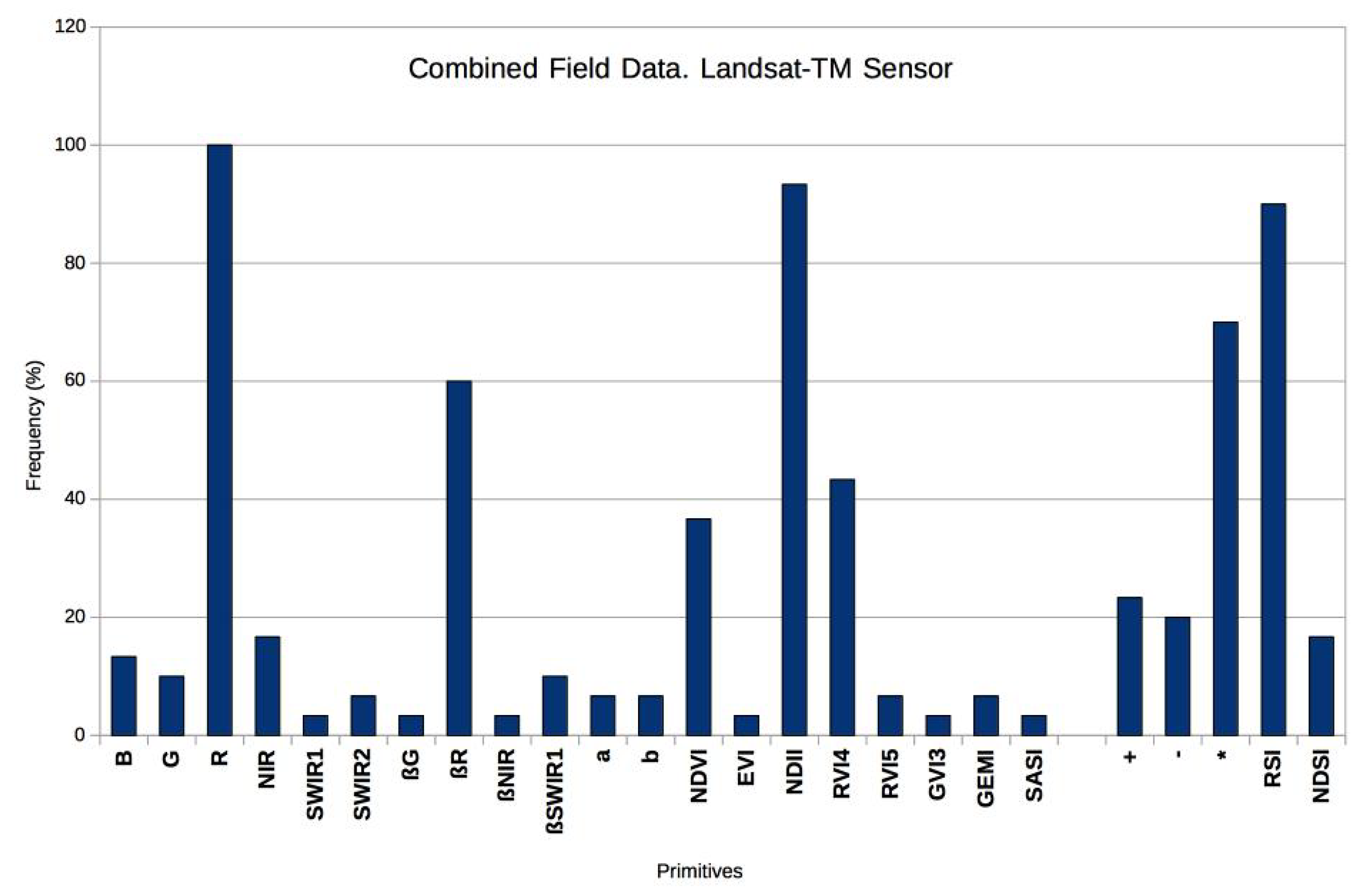
• Spectral bands represent the median value of the $3\times 3$ pixel window defined in Section 4.3, which was extracted from each satellite image band: Blue (B), Green (G), Red (R), Near-Infrared (NIR), Shortwave Infrared 1 (SWIR1), and Shortwave Infrared 2 (SWIR2).
• Spectral angles are the angles formed by each vertex in the electromagnetic spectrum for the satellite image [68]. For example, ${\beta }_G$ corresponds to the combination of pixels from the B, G, and R bands. The formula for this angle is:

  $${\beta }_G=co{s}^{-1}(\frac{a^2+b^2-c^2}{2ab})radians,$$

  (3)

  where a, b, and c are the Euclidean distances between the vertices of the angle formed by B, G, and R, respectively. Formula (3) is applied for each angle.
• Soil line parameters: This is the relationship between the R and NIR bands [70]. When these bands are graphed in a dispersion graph, they tend to group pixels above a numeric threshold, which is called the soil line. For this study, the slope and the intersect of the soil line are included in the primitives’ set as a and b in Table 3.
• Best-performing conventional VIs: The five better performing conventional VIs in Section 4.4 were selected. This performance is based in statistical significance [71], which is the probability that an index has a random correlation value $|r_{x,y}|$. For scientific research, the most common statistical significance value is 5%, which means that $|r_{x,y}|$ is significant if there is a 5% or less probability that the index has happened by chance. The statistical significance, $SS$, for the correlation coefficient, r, of a sample with N data is [71]:

  $$SS=\frac{r}{\sqrt{\frac{1-r^2}{N-2}}}$$

  (4)
  The field samples from both watersheds were used in this research, so the sample size for the training dataset was $N=102$. Therefore, correlation coefficients greater than 0.39 will be statistically significant for this experiment.
  Besides the five indices, it was decided to include the $NDVI$ and $EVI$ indices since these are the most used for scientific applications.
• Arithmetic operators: The function set is formed by the basic arithmetic operators (+, −, and ×) since these are the operators usually employed for VIs. For this work, division (/) is substituted by the compound operator Ratio Spectral Index (RSI) (see below).
• Compound operators: These represent complete arithmetic structures that have been previously defined. This research includes two of the most-employed indices, NDVI and RVI. The first structure is the Normalized Difference Spectral Index (NDSI) [72], which corresponds to NDVI; while the second structure is the Ratio Spectral Index (RSI), which corresponds to RVI. The definitions for these structures are:

  $$NDS{I}_{[i,j]}=\frac{R_i-R_j}{R_i+R_j},$$

  (5)

  $$RS{I}_{[i,j]}=\frac{R_i}{R_j},$$

  (6)

  where $R_k$ is the pixel reflectance value in band k.

4.5.2. Fitness Function

The GP algorithm defines a fitness function to determine how close a solution is to achieving the overall specification. For this study, it is based on the correlation coefficient $r_{x,y}$ between the C factor and each index. The absolute value of the correlation coefficient is employed because this application is looking for stronger correlations and not the direction. Therefore, the fitness function is defined as the maximum of the correlation coefficients:

$$Q=max(|r_{x,y}|),suchthat{r}_{x,y}=\frac{cov(x,y)}{var(x)var(y)}=\frac{E((x-{\mu }_x)(y-{\mu }_y))}{{\sigma }_x{\sigma }_y},$$

(7)

where E is the mathematical expectancy, $cov$ is the covariance, and $var$ is the variance. x represents the RUSLE’s C factor, while y is the VI generated by the GP algorithm.

4.5.3. Control Parameters and Stop Criteria

The control parameters for the GP algorithm will be described in Section 5.1.

Figure 3 shows the flow diagram of the methodology developed to generate the VIs that determine the RUSLE’s C factor. After processing the images, an initial population is randomly generated by combining the elements in the terminal and function sets. Then, each population individual is evaluated using the fitness function. The indices are then ordered according to the results of this function, where the best results are expected to survive and the worst will get discarded. At this point, the genetic recombination takes place, where the best syntactic trees, which represent an index, are combined using crossover and mutation operators. Finally, the next generation is formed by the best indices between the parents and children. These steps are successively executed until the maximum number of iterations is reached. The index with the greatest correlation value is considered the best one and is the new synthetic index. This new index is called the Genetic Programming for Vegetation Index, $GPV{I}_j$, where j is the iteration number that generated the index.

4.6. Results’ Evaluation

The results’ evaluation was performed according to the two stages used in machine learning theory: training and testing. Therefore, to evaluate the performance of each GPVI, the absolute difference between the correlation coefficients from the training stage and from the test stage was employed.

$$D=|r_{train}-r_{test}|$$

(8)

Besides evaluating each GPVI, each element that forms the primitive set was evaluated. This evaluation was done by using the Frequency Of Use (FOU) unit, which measures the capacity of a GP function to recognize patterns [25]. Counting the frequency of use of each element in the primitives’ set can be considered as an impact index to reflect the relative importance of the element. Thus, it was possible to determine the important components to measure the RUSLE’s C factor from satellite images.

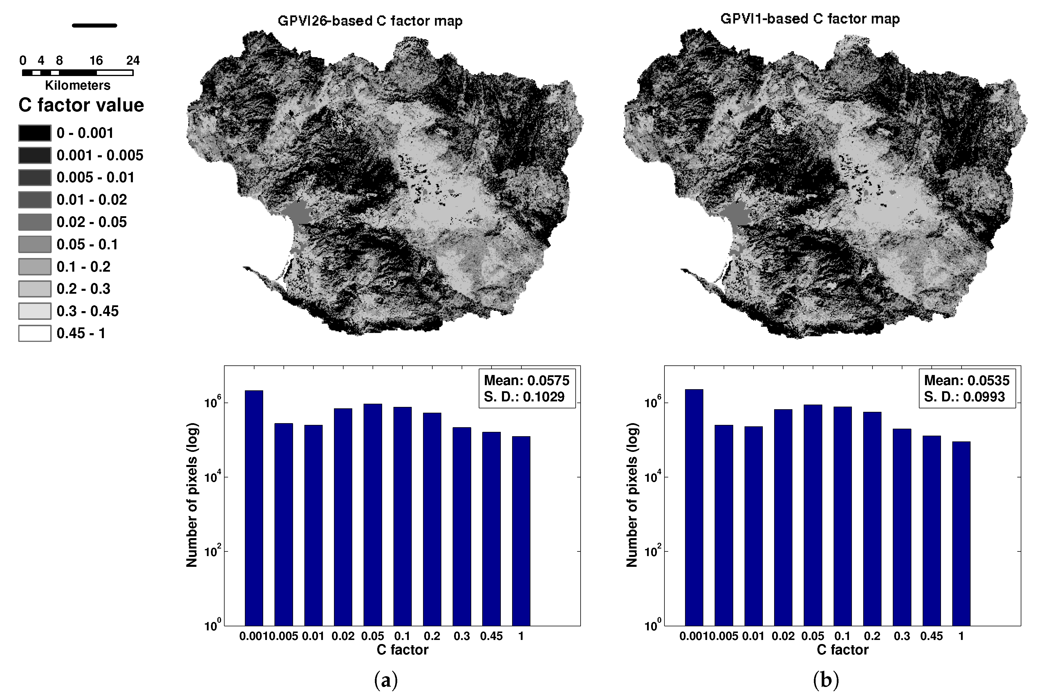
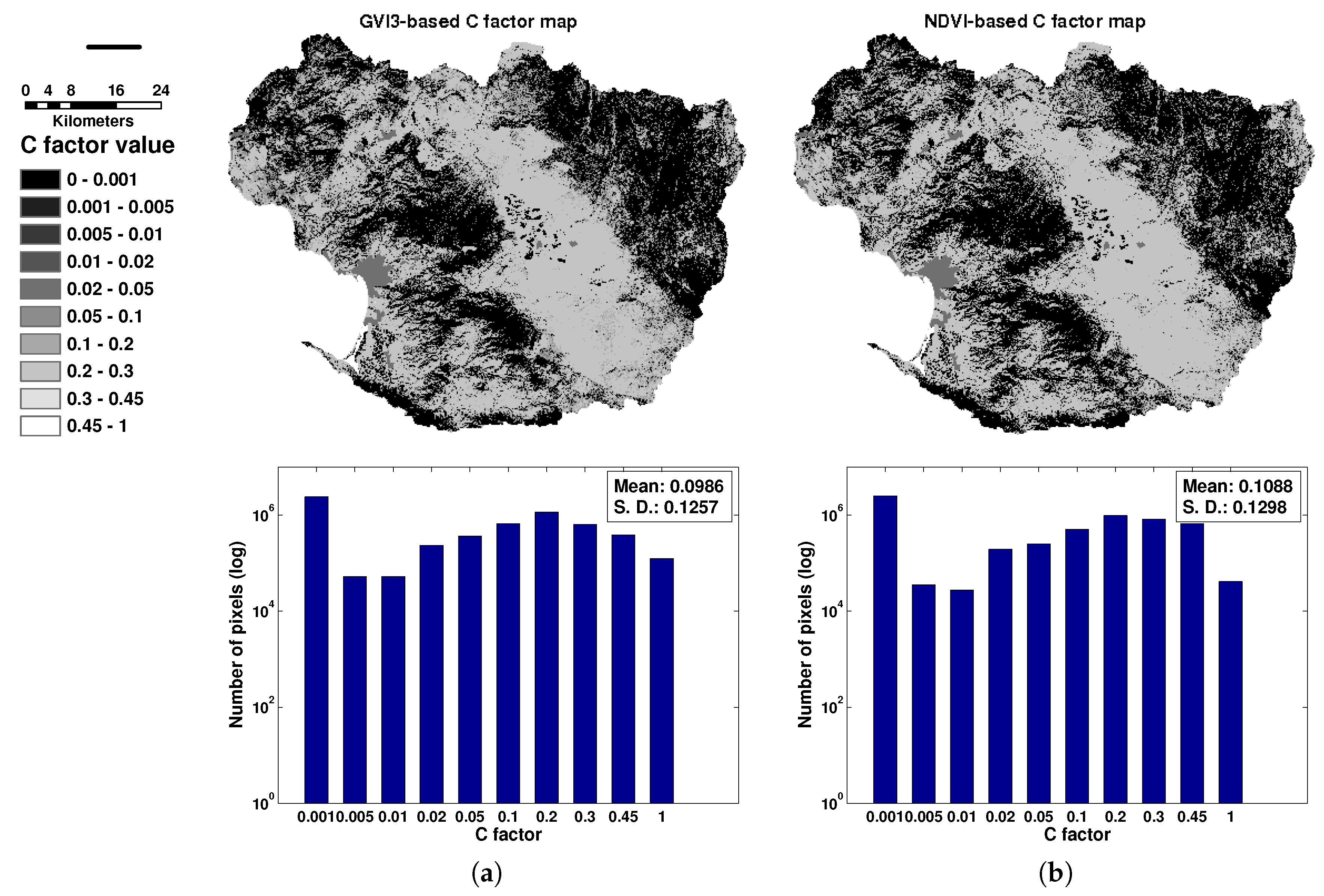
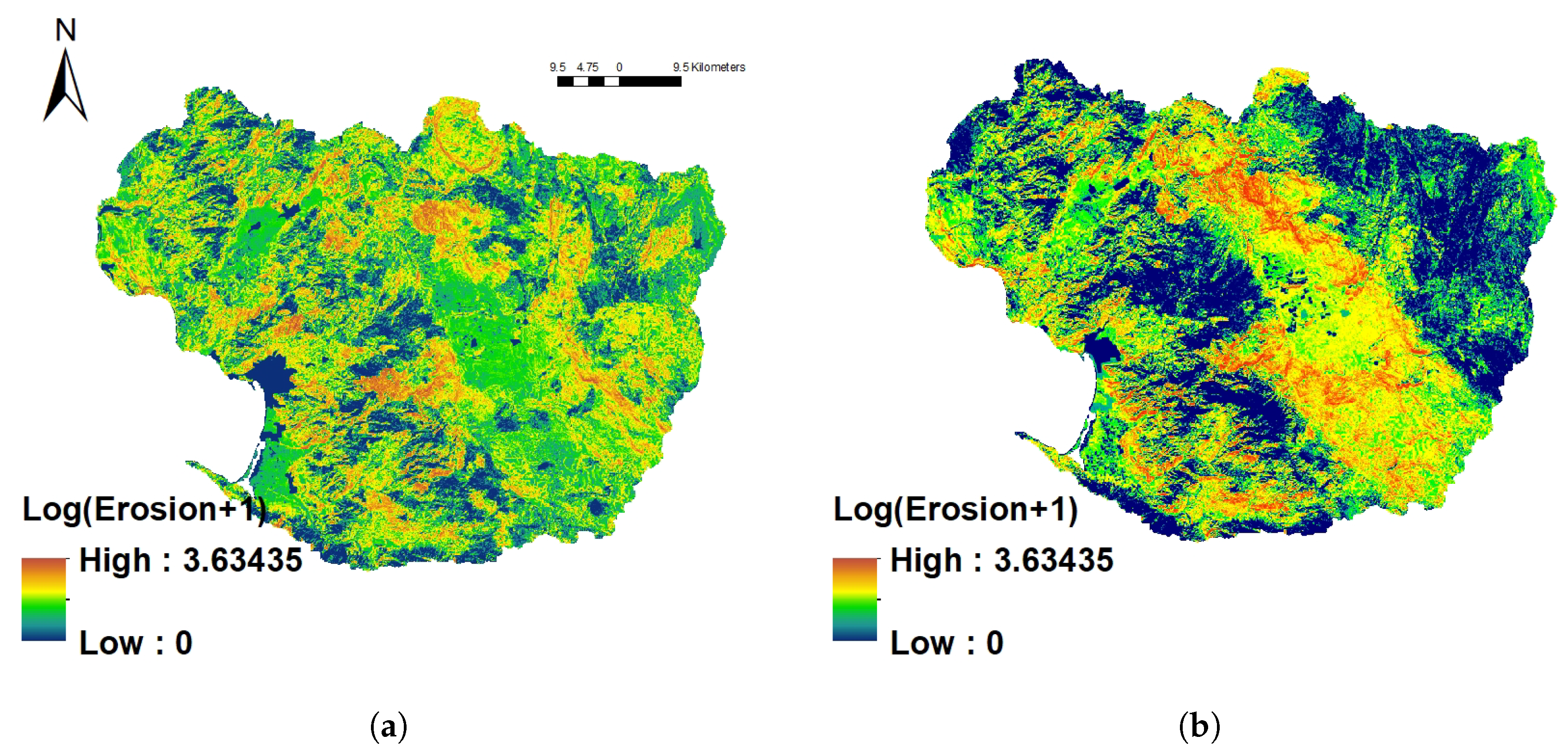
4.7. Generating the C Factor Map and the Erosion Map

Finally, a linear transformation was performed to convert each GPVI’s numerical scale to the C factor’s numerical scale. Thus, it is possible to produce a C factor map. Once the C factor map is generated, it can be used to feed the RUSLE’s model formula to obtain the erosion estimation (Equation (1)). Since the principal contribution of this research was the C factor methodology, the other RUSLE factors (R, K, L, S, and P) were determined by using the methodology proposed by [32] and the ArcGIS ©geographical information system (R, K, LS, and P calculations were performed based on Appendix A of [32], which is publicly available at http://www.esapubs.org/archive/appl/A017/052/appendix-A.htm). All the factors of the RUSLE model, except for C, remained unchanged throughout the experiments carried out in the next section. The numerical values used for each factor are reported in Section 5.3.

5. Experiments and Results

This section describes the experiments and results that measure the efficiency of the GP method developed for synthesizing VIs. In order to prove this efficiency, the GP algorithm needs to perform the following tasks correctly: (1) identify the satellite images’ spectral bands that predict the C factor; (2) generate C factor maps that match the field data; (3) generate erosion maps that approximate the erosion calculated from the C factor field data.

5.1. Implementing the GP Algorithm

The methodology described in Section 4.5 was implemented using MATLAB’s GPLab genetic programming toolbox [73]. GPLab has three main sections: initial population, new generation criteria, and population management. For each section, the toolbox requires the user to provide parameters to define the behavior of the algorithm. These parameters are described below.

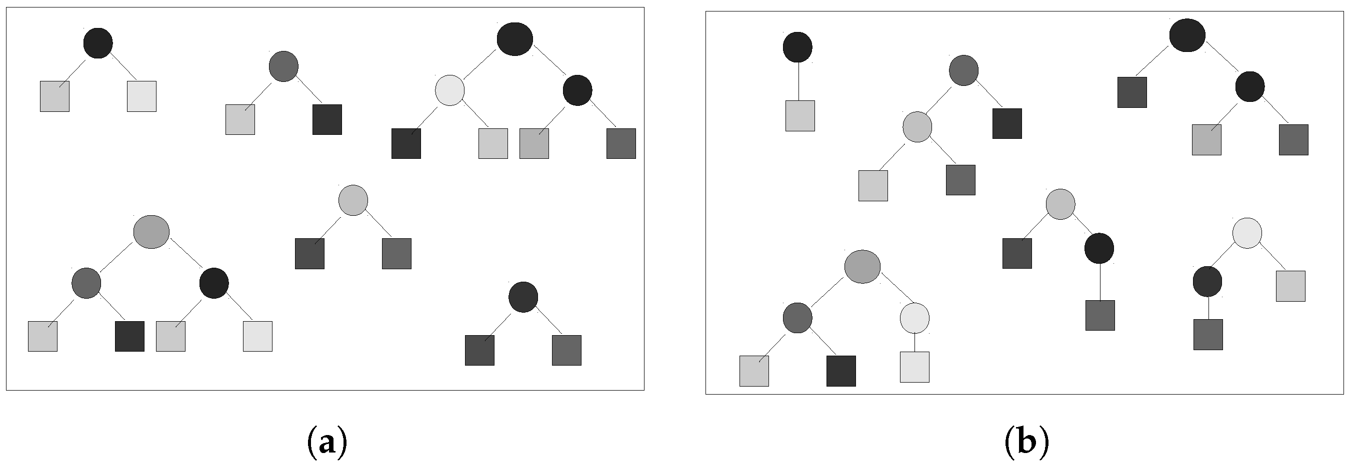
• Initial population: This section generates the initial population and evaluates it according to the fitness function (correlation coefficient) defined in Section 4.5. Population individuals may be generated according to one of three methods: full, grow, and ramped half-and-half. For the full method, the syntactic tree will include all possible nodes at each level (Figure 6a). The grow method generates a random number of nodes at each level, which may generate unbalanced trees (Figure 6b). The ramped Half-and-half method generates half of the tree using the full method and the other half using the grow method. This research employs this last method because it generates trees with a wide variety of sizes and shapes.
• New generation criteria: This section creates a new generation of individuals (children) by either applying genetic mutation operators or crossover (genetic reproduction) to the individuals of the previous population (parents). The following methods may be used to select the next generation’s parents: roulette, stochastic universal sampling, tournament, and lexicographic parsimony pressure tournament [35]. This last method is a special case of the tournament method where competing individuals with the same performance, following the fitness function, are selected according to the one that has the least complexity or the fewer number of nodes. This gives the advantage to simpler VIs that compete against conventional indices and is the reason why lexicographic parsimony pressure tournament was selected as the new generation method.
  Once the parents have been selected, either mutation or crossover is applied depending on a user-defined probability parameter. Usually, the mutation’s probability is lower than the crossover’s. For this experiment, the crossover probability was 0.7, while the mutation probability was 0.3. The new individuals were evaluated according to the fitness function, and then, these individuals and the best parents became the parents for the next generation. For this research, only the best individual in each generation was preserved for the next generation; this is called the elitist parameter. This procedure was repeated until a stop criteria was met, which for this research was when 50 generations had been produced. This number was employed because the algorithm stopped producing better individuals after 35 iterations.
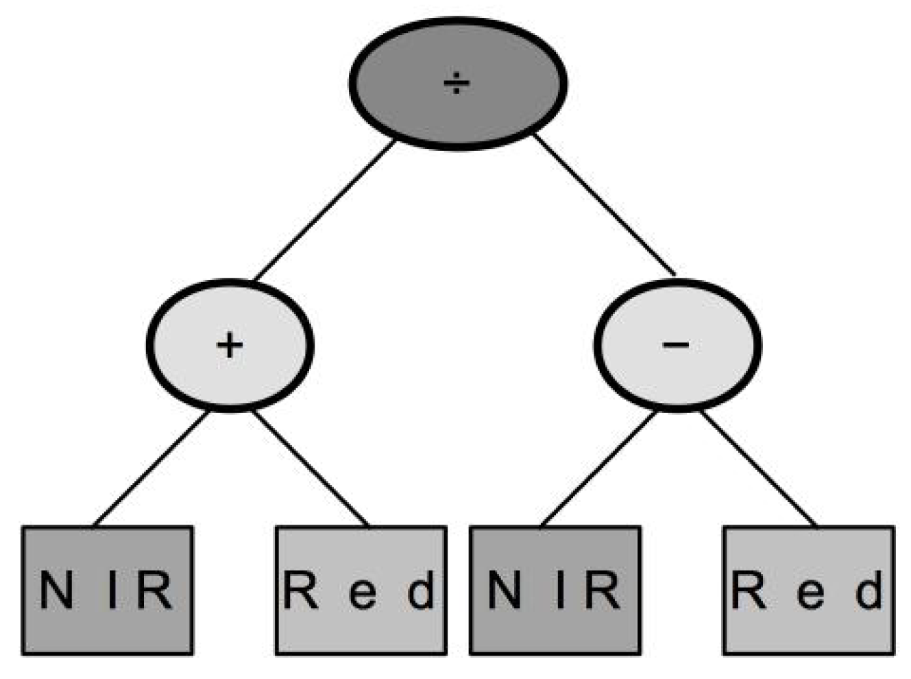
• Population management: Also called a code bloat in GP parlance, it limits the complexity of individuals. Three parameters are used to define this section: tree depth, maximum dynamic depth, and real maximum depth. If a new individual has a depth greater than the one defined at the beginning, the individual is automatically discarded regardless of the performance provided by the fitness function. This avoids an uncontrolled growth of the syntactic trees that generate the population. The tree depth has two possible values: strict means that the previous rule always applies, while dynamic allows one to preserve individuals that have a better performance than any other previous individual. The dynamic approach verifies that the new individual’s depth is greater than the maximum dynamic depth, but smaller than the real maximum depth. In such a case, the algorithm allows the new individual to survive and sets the maximum dynamic depth to the new individual’s depth value. If later on, there is a better individual with a smaller depth, the previous individual is discarded, and the maximum dynamic depth moves down to the new individual’s depth. In this research, individuals represent a VI in a syntactic tree. Figure 5 shows that the depth of the NDVI syntactic tree was three. The greater the depth of the tree, the greater the complexity; therefore, it is desirable that the GP-synthesized indices have a similar complexity to the conventional indices. Thus, the maximum dynamic depth was set to three, and the real maximum depth to four.

Multiple experiments were performed to determine some of the parameters employed in this study, while others used values that have been reported to provide good performance for different applications [35,74].

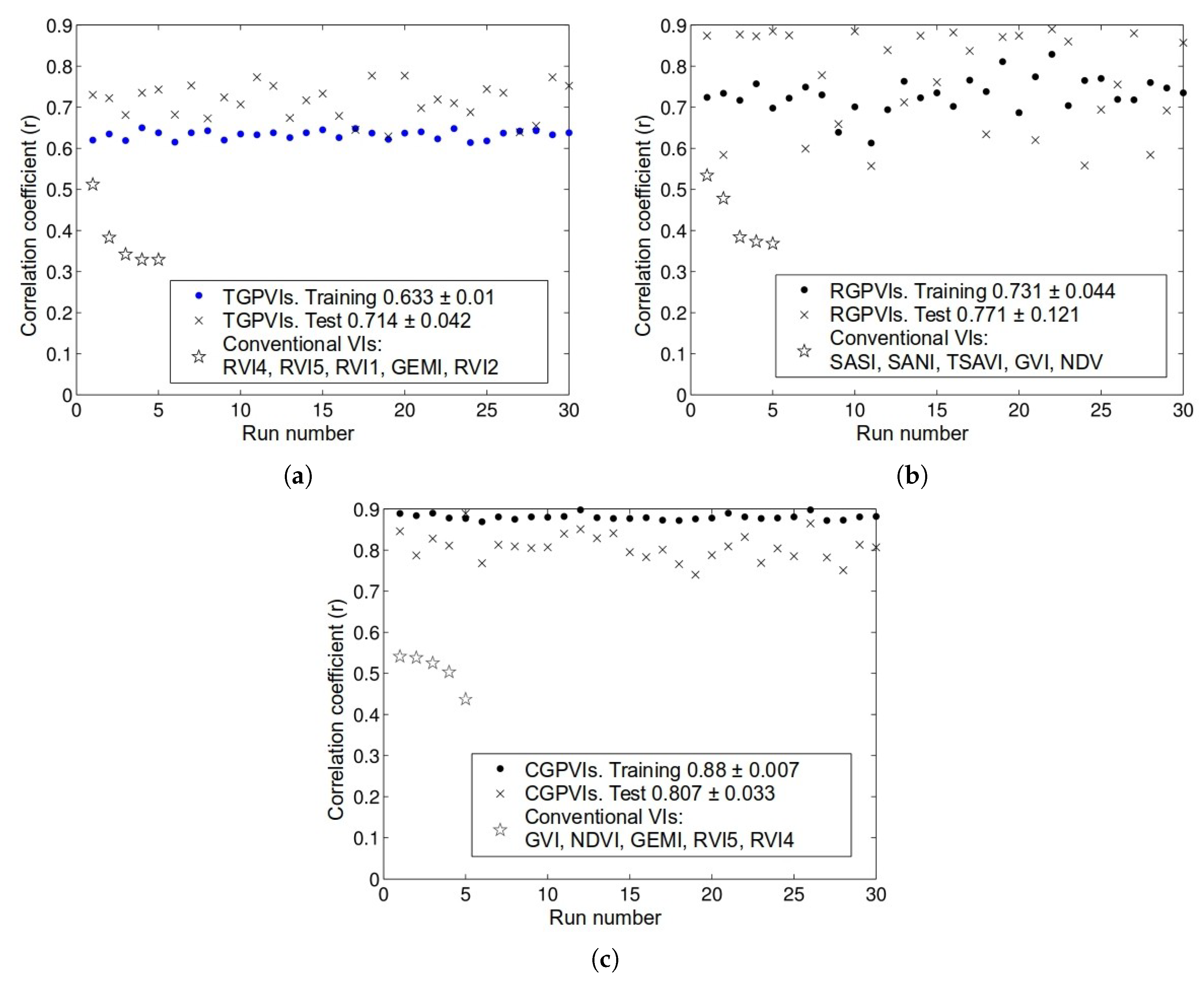
5.2. Methodology Performance Analysis

The current study proposes a methodology for synthesizing VIs that could be used in both watersheds. Two different hypothesis have been proposed to achieve this objective:

• The synthesized indices from one watershed produce a good approximation when applied to the other watershed.
• The combined synthesized indices from both watersheds produce a good approximation when they are later applied to each watershed.

5.2.1. First Hypothesis

The first hypothesis was tested using the procedure described in Section 4 to obtain 30 synthesized indices for each watershed, which have been reported in [29,30]. Figure 7a–c shows the correlation coefficient for the five best conventional indices for each watershed and their combined data, against their best-performing synthetic index in the training and test phases.

The 30 indices generated for Todos Santos were correlated with the field data from Rio Martin. Conversely, 30 indices generated for Rio Martin were correlated with data from Todos Santos.

Table 4. Confusion matrix showing the measured (correlation) performance $|r_{x,y}|$ when applying the Todos Santos synthesized indices to the Rio Martin watershed, and vice versa.

	Todos Santos	Rio Martin
Todos Santos	0.633 ± 0.01	0.323 ± 0.010
	Max. 0.65	Max. 0.363
	Min. 0.614	Min. 0.290
Rio Martin	0.329 ± 0.11	0.731 ± 0.044
	Max. 0.401	Max. 0.829
	Min. 0.137	Min. 0.613

shows the confusion matrix generated by the data from both watersheds. The matrix’s main diagonal contains the performance of the indices generated using the original field data from each dataset. The other elements show the performance of the Todos Santos’ index in Rio Martin (Row 1, Column 2) or the performance of the Rio Martin’s index in Todos Santos (Row 2, Column 1). These correlation values are low and suggest that the first hypothesis is false. Therefore, it is possible to conclude that indices generated from one of these watersheds may produce low performance (correlation) when applied to the other watershed.

5.2.2. Second Hypothesis

This hypothesis was tested using the methodology introduced in Section 4. The training phase employed 102 sample points: 75 from Todos Santos and 27 from Rio Martin. While the testing phase used 44 sample points: 31 from Todos Santos and 13 from Rio Martin.

The satellite image corrections described in Section 4.2 were performed, and these images were associated with the corresponding sample points (Section 4.3). Then, the 30 conventional indices from Table 2 were correlated to the field data from each watershed, as described in Section 4.4. The 10 best-performing indices are included in

Table 5. Conventional vegetation indices (Table 2) with the best performance for the combined data from both watersheds. Performance was measured by using the correlation factor ($|r_{x,y}|$).

Index	GVI3	NDVI	GEMI	RVI5	RVI4	SASI	NDII	OSAVI	RVI1	TSAVI
$|r_{x,y}|$	0.541	0.538	0.525	0.503	0.437	0.349	0.341	0.328	0.309	0.302

. $GVI3$ had the best performance, followed by $NDVI$, $GEMI$, and the two indices derived from $RVI$: $RVI5$ and $RVI4$. Two indices from the $SAVI$ family were also included: $TSAVI$ and $OSAVI$. Importantly, the performance of the conventional indices was low, when correlated to the C factor: the average $|r_{x,y}|$ for the top 10 indices was 0.417 ± 0.101.

Table 5 shows that no strong correlation values were found between the most-employed VIs and the field data. This is expected in arid areas since VIs have good correlation with abundant and green vegetation, but as the green vegetation decreases, so do the correlation values [4]. However, the state of vegetation is not that important for erosion models, since dry vegetation provides almost the same protection as green vegetation [75]. Even with these obstacles, VIs have been widely employed to extrapolate C factor values for different regions [32,75,76,77,78].

The seven best VIs from Table 5 were included in the primitive set. The EVI index was also included in this set because it is widely employed in scientific applications. Then, the algorithm was executed 30 times, and in each execution, the best individual was allowed to continue and was named the Combined data Genetic Programming for Vegetation Index in execution j, $CGPV{I}_j$.

Table 6. Synthesized VIs for the GP method using the combined data from both watersheds. Performance was measured through the correlation factor ($|r_{x,y}|$).

Index	Formula	$|{\mathit{r}}_{\mathit{train}}|$	$|{\mathit{r}}_{\mathit{test}}|$	Dif.
CGPVI1	$RSI(RSI(b+R,RSI(NDVI,R)),G+2·NDII)$	0.887	0.849	0.037
CGPVI2	$(NDII+Bl)\times RSI({\beta }_R,NDII)\times R\times {\beta }_R\times {\beta }_R$	0.884	0.787	0.097
CGPVI3	$(R-NDII)\times (GEMI-NDII)\times RSI(B,EVI)$	0.890	0.828	0.061
CGPVI4	$RSI(RVI4\times R,NDII)\times {\beta }_R\times {\beta }_R\times R\times RVI4$	0.878	0.811	0.067
CGPVI5	${\beta }_{SWIR1}\times {\beta }_{SWIR1}\times R\times G\times (R-G)$	0.861	0.899	0.038
CGPVI6	$RSI(RSI(RSI(R,NDII),GEMI-m),NDVI)$	0.869	0.768	0.102
CGPVI7	$RVI4\times RVI4\times {\beta }_R\times R\times R\times RSI({\beta }_R,NDII)$	0.881	0.813	0.068
CGPVI8	$R\times R\times RSI({\beta }_R,NDII)\times RVI4\times RVI4$	0.875	0.809	0.066
CGPVI9	$RSI({\beta }_R,NDII)\times R\times R\times {\beta }_R\times {\beta }_R\times RVI4$	0.881	0.805	0.075
CGPVI10	$RVI4\times RVI4\times R\times RSI({\beta }_R,NDII)\times {\beta }_R\times {\beta }_R$	0.880	0.807	0.073
CGPVI11	$RSI(RSI(R,NDVI),RVI4)\times RSI(RSI(R,RVI4),RVI4)$	0.882	0.840	0.042
CGPVI12	$NDSI(NDII,SWIR1)\times R\times SWIR1\times NDSI(NDII,SWIR1)\times$ $NDSI({\beta }_{SWIR1},RVI5)$	0.898	0.851	0.048
CGPVI13	$NDSI(R,NDII)\times B\times SWIR2$	0.879	0.829	0.050
CGPVI14	$NDSI(RSI(NDII+R,RSI(NDII,R)),{\beta }_G)$	0.878	0.840	0.038
CGPVI15	$(RVI4-2·NDVI)\times R\times RSI({\beta }_R,NDII)$	0.877	0.795	0.083
CGPVI16	${\beta }_R\times {\beta }_R\times {\beta }_R\times RSI(G,NDII)\times R$	0.879	0.783	0.096
CGPVI17	$RSI(R\times R\times RVI4\times {\beta }_R,NDII)$	0.873	0.801	0.072
CGPVI18	$RSI(RSI(R,NDVI),NDII)-RVI5-{\beta }_R-NDII$	0.872	0.766	0.105
CGPVI19	$RSI(RSI(SWIR2,NDVI),NDVI)+RSI(RSI(R,NDII),NDVI)$	0.876	0.740	0.136
CGPVI20	$RSI(RSI({\beta }_R,NDII)+RSI({\beta }_{SWIR1},NDVI)+RSI(RSI(NIR,R),R)$	0.878	0.788	0.090
CGPVI21	$NDSI(R,NDII)\times B\times NDSI(NIR,NDII\times R$	0.890	0.809	0.081
CGPVI22	${\beta }_R^2\times m\times R\times (RSI(R,NDII)+{\beta }_R)$	0.881	0.832	0.049
CGPVI23	$RSI(RSI({\beta }_R,RSI(NDII,R)),RSI(RSI(NDVI,RVI4),{\beta }_R))$	0.877	0.769	0.108
CGPVI24	$RSI({\beta }_R\times RVI4,NDII)\times {\beta }_R^2\times R\times R$	0.878	0.804	0.074
CGPVI25	$RSI(R,NDVI)\times (SASI+{\beta }_R)\times ({\beta }_R+RSI(NIR,NDII))$	0.881	0.785	0.096
CGPVI26	$NDSI(NDSI(GVI3\times R,NDII),NDSI(R,RSI(NDII,R)))$	0.898	0.865	0.033
CGPVI27	$RSI(RSI({\beta }_R,RSI(NIR,R)),RSI(NDII,R))$	0.872	0.782	0.090
CGPVI28	$RSI(RSI(RSI(RVI4,NDVI),RSI(b,R)),RSI(NDTI,$ $RSI(RVI4,{\beta }_{NIR})))$	0.873	0.751	0.122
CGPVI29	$RVI4\times RVI4\times RSI({\beta }_R,NDII)\times R\times R\times {\beta }_R\times {\beta }_R$	0.881	0.813	0.068
CGPVI30	$(RVI4-NDVI)\times (RVI4\times R\times {\beta }_R\times {\beta }_R\times RSI({\beta }_R,NDII)$	0.882	0.807	0.075

shows the performance of each $CGPV{I}_j$ produced by the GP algorithm. This performance was the difference between the $r_{train}$ and $r_{test}$ correlation coefficients. From Table 5 and Table 6, it is possible to determine that indices synthesized by the GP algorithm had a better performance than the conventional ones. This result was supported by the average $r_{train}$ value for the CGPVIs (0.88 ± 0.007) and the average $r_{x,y}$ for the top ten conventional VIs (0.417 ± 0.101). Moreover, all the CGPVIs in Table 6 were statistically significant [71] and produced a better correlation coefficient than the conventional index with the best coefficient, as can be seen in Figure 7c.

The importance of each element in the primitive set was evaluated by means of the FOU unit. Figure 8 shows that the most-employed spectral band was R, since it is present in all the indices. The second most-employed bands were $SWIR1$ and $SWIR2$, which are implicitly used in the conventional NDTI (93.33%). Moreover, considering that $RVI4$’s percentage was 43.33% and the ones for $SWIR1$ and $SWIR2$, when used explicitly, were 3.33% and 6.67%, respectively, it is possible to conclude that $SWIR1$ and $SWIR2$ were also employed by the 30 GP-synthesized indices. $NIR$ was the fourth most-employed spectral band, as it was employed in 29 synthetic indices (90%) when both explicit and implicit occurrences were counted. These percentages allow hypothesizing that R, $NIR$, $SWIR1$, and $SWIR2$ are the best spectral bands to approximate the C factor from the satellite images; especially when considering that the two remaining spectral bands, B and G, do not have high FOU percentages, 20% and 60%, respectively. These results suggest that the GP algorithm is able to define a function using the four most-cited bands to approximate the C factor [16,50,64,68,79]. This experiment confirms an observation previously published in [29]: NDVI, the most-employed index in other applications, had a low FOU value: 36.330.

For the elements in the function set, the most-used operator was $RSI$ with 90%. The fact that the GP algorithm favored the $RSI$ structure in this experiment supports previous arguments by other researchers [72,80], which concluded that this ratio diminishes the effects of the noise produced by the terrain’s topography, the position of the Sun with respect to the position of the satellite, and other atmospheric conditions. However, the $NDSI$ operator FOU percentage was 16.66%, which is low compared with the results obtained when data from both watersheds were employed separately [29,30]. Nevertheless, it must be considered that the conventional $NDII$(93.33%) employed the $NDSI$ structure.

In order to obtain the erosion rate in Todos Santos, it was necessary to build C factor maps using the best-evaluated synthetic indices. However, the numeric scale for these indices had a different range from the C factor’s. For example, $NVDI$’s range is −1–1, while the C factor scale’s range is 0–1. MATLAB’s cftool was employed to perform linear transformations between the different VIs and the C factor. This tool recursively fits data points to a line, thus allowing one to transform values between different numeric ranges. The transformation provided by this tool was employed to generate C factor maps for the best CGPVI indices.

The two best-performing indices were selected to analyze their effectiveness by means of the C factor and erosion maps. The best solution should be the one that produces the smallest difference for Equation (8). Then, following the data from the last column of Table 6, the best indices were $CGPVI26$ and $CGPVI1$. The equation for these indices was applied to the satellite image (Figure 9). The adjustment criteria proposed by [32] were employed to include non-vegetation coverings in these maps: negative C values were set to zero; values greater than or equal to 0.45 in agricultural areas were set to $C=1.0$ (recently-plowed soil); all bodies of water had a value of $C=0$; finally, heavily-paved urban areas were set to $C=0.02$. To complete this analysis, the comparison included the C factor maps from the best-performing conventional indices: $GVI3$ and $NDVI$ (Figure 10). Moreover, the adjustment criteria proposed by [32] were also employed in these maps, in order to include non-vegetation coverings. The range for these maps was [0.0, 1.0], and their averages were $0.0575\pm 0.1029$ for CGPVI26 and $0.0535\pm 0.0993$ for CGPVI1. Conversely, the average for the conventional indices’ maps was $0.0986\pm 0.1257$ and $0.1088\pm 0.1298$, respectively. To ease the comparison of these results, the C values have been divided into ten different intervals.

Figure 9 and Figure 10 show that C factor maps produced by the $CGPVI26$, $CGPVI1$, $GVI3$, and $NDVI$ indices. At first sight, these maps look similar and reflect the conditions of the main vegetation coverings. However, analysis of the histogram for each map reveals differences in the number of pixels in each classification. The histograms from Figure 9 have two maximum values in the first and fifth interval. This suggests that a large portion of the area had C values in the [0, 0.001] and [0.02, 0.05] ranges, which corresponds to abundant vegetation coverings: between 80% and 90% of the superficial area, according to Table 10 in the USLE’s protocol [8]. These results match the field observations in the Todos Santos watershed, which is predominantly covered by shrubs (Figure 1b).

In contrast, the maps for the $GVI3$ and $NDVI$ indices (Figure 10) had maximum values in the first and seventh classification, which means that a large portion of the watershed had C values in the [0, 0.001] and [0.1, 0.2] ranges. This latter value corresponds to a semi-sparse cover, which occupies between 30% and 40% of the surface and could be explained by $NDVI$’s low performance for detecting dry vegetation, which causes an over-estimation of the C values. The same effect can be seen in Figure 10b, where $NDVI$ was not able to detect dry grassland at the center of the watershed, contradicting the information from Figure 1b. In contrast, the maps in Figure 9 were able to record a more diverse set of C values for this area because these indices employ the shortwave infra-red bands (SWIR1 and SWIR2), which distinguish between dry vegetation and bare soil [68]. Following these observations, it is possible to assert that the two CGPVI indices analyzed were able to distinguish between areas of dry vegetation and areas of bare soil because they employed the combined information of the best spectral bands for calculating the C factor: NIR, R, SWIR1, and SWIR2.

5.3. Erosion Rate Analysis for the Todos Santos Watershed

This section analyzes the erosion maps generated by the indices synthesized in the previous section for the Todos Santos watershed. A similar analysis, but for the Rio Martin watershed, was previously reported in [30], where the synthetic indices were employed to evaluate erosion caused by coal mining.

After synthesizing the new indices and selecting the best ones for generating the C factor’s map, an erosion map can be finally produced. The RUSLE’s R factor was obtained by using the method by [81], which estimates this factor using a regression analysis from the annual precipitation record in the watershed. These records were obtained for Mexico’s Comisión Nacional del Agua (CNA) [38]. Thus, the R value recorded for the whole watershed was 51,000 MJ·mm·km${}^{-2}$·h${}^{-1}$·year${}^{-1}$. The L and S factors were simultaneously obtained from a digital elevation model, following the procedure by [82] and [83]. The digital model employed for this research was produced by Mexico’s Instituto Nacional de Estadística y Geografía (INEGI) [84]. The K factor was set using the soil texture method described in the RUSLE protocol [7]. For Todos Santos, the soil texture data were obtained from INEGI’s soil profile reports [85]. The P factor was set to a value of one for the whole watershed, since soil conservation practices for this region are limited.

For each of the erosion maps, the RUSLE’s factors R, L, S, K, and P were defined as described before. However, the C factor varies according to the factor maps generated previously. This is shown in Figure 11, which includes the erosion maps obtained from the $CGPVI1$ and $GVI3$ indices. $CGPVI1$ was the synthetic index with the best performance, while $GVI3$ was the best-evaluated conventional index.

Table 7. Average and standard deviation for the erosion rate from the sampling points for the training set. Each row shows a different method to calculate C.

Method employed to calculate C	Erosion (Mg·km${}^{-2}$·year${}^{-1}$)
Field data	$76.6\pm 153.6$
Indices generated from field data from the Todos Santos and Rio Martin watersheds
CGPVI26	$99.5\pm 216.8$
CGPVI1	$111.1\pm 278.7$
GVI3	$376.5\pm 780.3$
Spectral classification method
Spectral classification method	$170.6\pm 358.8$

shows the erosion rates obtained from the sampling points in Todos Santos using the different C factor maps. The first row shows the average erosion rate from the field data. The best approximations to these data were produced by the synthetic vegetation indices: the average erosion rate from the CGPVI26 was $99\pm 217$; while for CGPVI1, it was $111\pm 279$. These erosion rates were not as high as the one from the best-performing conventional index, $GVI3$, which was more than five-times the average rate from real data ($377\pm 780$). The last row of Table 7 shows the erosion rate obtained by applying a spectral classification method to get the C factor. A land cover map of the study area was obtained from the Comisión Nacional Forestal (CONAFOR) [37], and it is shown in Figure 1b. C values’ labels were assigned according to vegetative covers in Table 10 from the USLE protocol [8]. It can be seen that the classification cover method yielded an erosion rate that was twice the value obtained from the field data.

The classification method for the land cover, which produced an average erosion rate equal to $170\pm 358$, was not as good as the synthetic indices. Among them, CGPVI26 had the best fit, since it produced an average rate closer to the one obtained from the field data. This difference can be seen in Figure 9 and Figure 10, where the map produced by CGPVI26 had greater spatial variability than the one for GVI3. For example, GVI3 was not able to detect the dry grassland area in the south portion of the Ojos Negros valley and treated it as bare soil, which produced a high C value; while CGPVI26 was able to assign different C values for this same area and produced a more precise erosion map.

6. Conclusions

The field data from the Todos Santos and Rio Martin watersheds were combined into a single dataset, which was then correlated with satellite images. The best-performing indices were $CGPVI26$, $CGPVI1$, and $CGPVI14$, which were able to obtain $r_{x,y}$ values of 0.898, 0.887, and 0.878, respectively. These indices produced better results than the best-performing conventional indices, which were GVI3 with $r_{x,y}=0.541$ and NDVI with $r_{x,y}=0.538$. The results indicate that these indices produced erosion rates with greater values than the real ones. For example, the erosion maps based on CGPVI26 produced an average rate of $99.5\pm 216.8$ Mg·km${}^{-2}$·year${}^{-1}$, while the rate measured by the field experiment was $76.6\pm 153.6$ Mg·km${}^{-2}$·year${}^{-1}$.

These results suggest that genetic programming is a useful tool to discover the spectral band combinations that identify the main elements to estimate the RUSLE’s C factor. The methodology employed in this research was able to determine that bands R, NIR, SWIR1, and SWIR2 were the most appropriate to calculate the C factor. The GP algorithm was also able to identify RSI and NDSI arithmetic structures, which have been used before to diminish the effects of the noise caused by topography, variations of the angle between the Sun and a satellite, and the atmospheric conditions [72,80].

Another conclusion from this research is about the generality of the methodology developed to identify a C factor approximation. A first experiment employed field data with the objective of finding if the synthesized indices for one watershed could be effective when applied to the other one. The results of this experiment suggest that this is not possible. This suggests that, although both watersheds in this research have similar topography and climate, their particular characteristics are too complex to allow grouping them using a single vegetation index.

Nevertheless, this work shows that combining the field data from two watersheds in a single dataset yields the design of VIs that obtain better correlation with the C factor than VIs synthesized from just one watershed. Hence, it is concluded that it is necessary to continue exploring the applicability of the proposed methodology in other watersheds that have different conditions. As this methodology is applied to different areas, it might be possible to identify a pattern of the elements and arithmetic structures that produce the best indices. This information would give certainty about those indices, preventing the need to synthesize new indices. A validated index could be executed as often as required. This fact opens the possibility, as future work, of applying this methodology to novel soil erosion models, such as G2 [86] and others.

This paper’s contribution improves on previous methods to calculate RUSLE’s C factor and allows generating more precise erosion maps, which should motivate others to continue exploring the use of genetic programming for remote sensing applications.

References

- Vrieling, A. Satellite remote sensing for water erosion assessment: A review. CATENA 2006, 65, 2–18. [Google Scholar] [CrossRef]
- Brady, N.C.; Weil, R.R. The Nature and Properties of Soils, 4th ed.; Pearson-Prentice Hall: Upper Saddle River, NJ, USA, 2008; p. 550. [Google Scholar]
- Ananda, J.; Herath, G. Soil erosion in developing countries: A socio-economic appraisal. J. Environ. Manag. 2003, 68, 343–353. [Google Scholar] [CrossRef]
- de Jong, S. Applications of Reflective Remote Sensing for Land Degradation Studies in a Mediterranean Environment. Ph.D. Thesis, Universiteit Utrecht, Utrecht, The Netherlands, 1994. [Google Scholar]
- van der Meer, F.D.; de Jong, S.M. Imaging Spectrometry. Basic Principles and Prospective Applications; Kluwer Academic Publishers: Dordrecht, The Netherlands, 2001. [Google Scholar]
- Flanagan, D.C.; Nearing, M.A. USDA—Water Erosion Prediction Project. Hillslope Profile and Watershed Model Documentation; NSERL Report; USDA-ARS National Soil Erosion Research Laboratory: Washington, DC, USA, 1995; Volume 10.
- Renard, K.; Foster, G.; Weesies, G. Predicting Soil Erosion by Water: A Guide to Conservation Planning with the Revised Universal Soil Loss Equation (RUSLE); U.S. Department of Agriculture: Washington, DC, USA, 1996; Volume 703.
- Wischmeier, W.; Smith, D. Predicting Rainfall Erosion Losses: A Guide to Conservation Planning; U.S. Department of Agriculture: Washington, DC, USA, 1978; Volume 537.
- Borrelli, P.; Robinson, D.A.; Fleischer, L.R.; Lugato, E.; Ballabio, C.; Alewell, C.; Meusburger, K.; Modugno, S.; Schütt, B.; Ferro, V.; et al. An assessment of the global impact of 21st century land use change on soil erosion. Nat. Commun. 2017, 8, 2013. [Google Scholar] [CrossRef] [PubMed]
- Inoue, Y.; Olioso, A. Estimating dynamics of ecosystem CO2 flux and biomass production in agricultural field by synergy of process model and remotely sensed signature. J. Geophys. Res. Atmos. 2006, 111. [Google Scholar] [CrossRef]
- Kurzweil, R. The Age of Intelligent Machines; MIT Press: Cambridge, MA, USA, 1990. [Google Scholar]
- Congalton, R.G.; Balogh, M.; Bell, C.; Green, K.; Milliken, J.A.; Toman, R. Mapping and Monitoring Agricultural Crops and Other Land Cover in the Lower Colorado River Basin. Photogramm. Eng. Remote Sens. 1998, 64, 1107–1113. [Google Scholar]
- Asner, G.P.; Lobell, D.B. A biogeophysical approach for automated SWIR unmixing of soils and vegetation. Remote Sens. Environ. 2000, 74, 99–112. [Google Scholar] [CrossRef]
- Benz, U.C.; Hofmann, P.; Willhauck, G.; Lingenfelder, I.; Heynen, M. Multi-resolution, object-oriented fuzzy analysis of remote sensing data for GIS-ready information. ISPRS J. Photogramm. Remote Sens. 2003, 58, 239–258. [Google Scholar] [CrossRef]
- Guerschman, J.P.; Hill, M.J.; Renzullo, L.J.; Barrett, D.J.; Marks, A.S.; Botha, E.J. Estimating fractional cover of photosynthetic vegetation, non-photosynthetic vegetation and bare soil in the Australian tropical savanna region upscaling the EO-1 Hyperion and MODIS sensors. Remote Sens. Environ. 2009, 113, 928–945. [Google Scholar] [CrossRef]
- Tucker, C.J. Red and Photographic infrared linear combinations for monitoring vegetation. Remote Sens. Environ. 1979, 8, 127–150. [Google Scholar] [CrossRef]
- Van der Knijff, J.; Jones, R.; Montanarella, L. Soil Erosion Risk Assessment in Italy; European Soil Bureau, European Commission: Brussels, Belgium, 1999. [Google Scholar]
- Van der Knijff, J.; Jones, R.; Montanarella, L. Soil Erosion Risk Assessment in Europe; European Soil Bureau, European Commission: Brussels, Belgium, 2000. [Google Scholar]
- Mondal, A.; Khare, D.; Kundu, S. Impact assessment of climate change on future soil erosion and SOC loss. Nat. Hazards 2016, 82, 1515–1539. [Google Scholar] [CrossRef]
- Kourgialas, N.N.; Koubouris, G.C.; Karatzas, G.P.; Metzidakis, I. Assessing water erosion in Mediterranean tree crops using GIS techniques and field measurements: The effect of climate change. Nat. Hazards 2016, 83, 65–81. [Google Scholar] [CrossRef]
- Gupta, S.; Kumar, S. Simulating climate change impact on soil erosion using RUSLE model—A case study in a watershed of mid-Himalayan landscape. J. Earth Syst. Sci. 2017, 126, 43. [Google Scholar] [CrossRef]
- Amanambu, A.C.; Li, L.; Egbinola, C.N.; Obarein, O.A.; Mupenzi, C.; Chen, D. Spatio-temporal variation in rainfall-runoff erosivity due to climate change in the Lower Niger Basin, West Africa. Catena 2019, 172, 324–334. [Google Scholar] [CrossRef]
- Saadoud, D.; Hassani, M.; Peinado, F.J.M.; Guettouche, M.S. Application of fuzzy logic approach for wind erosion hazard mapping in Laghouat region (Algeria) using remote sensing and GIS. Aeolian Res. 2018, 32, 24–34. [Google Scholar] [CrossRef]
- Mangiarotti, S.; Mazzega, P.; Jarlan, L.; Mougin, E.; Baup, F.; Demarty, J. Evolutionary bi-objective optimization of a semi-arid vegetation dynamics model with NDVI and σ0 satellite data. Remote Sens. Environ. 2008, 112, 1365–1380. [Google Scholar] [CrossRef]
- Makkeasorn, A.; Chang, N.; Li, J. Seasonal change detection of riparian zones with remote sensing images and genetic programming in a semi-arid watershed. J. Environ. Manag. 2009, 90, 1069–1080. [Google Scholar] [CrossRef] [PubMed]
- Smith, M.O.; Ustin, S.L.; Adams, J.B.; Gillespie, A. Vegetation in deserts: I. a regional measure of abundance from multispectral images. Remote Sens. Environ. 1990, 31, 1–26. [Google Scholar] [CrossRef]
- Rizeei, H.M.; Saharkhiz, M.A.; Pradhan, B.; Ahmad, N. Soil erosion prediction based on land cover dynamics at the Semenyih watershed in Malaysia using LTM and USLE models. Geocarto Int. 2016, 31, 1158–1177. [Google Scholar] [CrossRef]
- Yang, X. Deriving RUSLE cover factor from time-series fractional vegetation cover for hillslope erosion modelling in New South Wales. Soil Res. 2014, 52, 253–261. [Google Scholar] [CrossRef]
- Puente, C.; Olague, G.; Smith, S.V.; Bullock, S.H.; Hinojosa-Corona, A.; González-Botello, M.A. A genetic programming approach to estimate vegetation cover in the context of soil erosion assessment. Photogramm. Eng. Remote Sens. 2011, 77, 363–376. [Google Scholar] [CrossRef]
- Trabucchi, M.; Puente, C.; Comin, F.A.; Olague, G.; Smith, S.V. Mapping erosion risk at the basin scale in a Mediterranean environment with opencast coal mines to target restoration actions. Reg. Environ. Chang. 2012, 12, 675–687. [Google Scholar] [CrossRef]
- Nicu, I.C. Application of analytic hierarchy process, frequency ratio, and statistical index to landslide susceptibility: An approach to endangered cultural heritage. Environ. Earth Sci. 2018, 77, 79. [Google Scholar] [CrossRef]
- Smith, S.V.; Bullock, S.H.; Hinojosa-Corona, A.; Franco-Vizcaíno, E.; Escoto-Rodríguez, M.; Kretzschmar, T.G.; Farfán, L.M.; Salazar-Ceseña, J.M. Soil Erosion and Significance for Carbon Fluxes in a Mountainous Mediterranean-Climate Watershed. Ecol. Appl. 2007, 17, 1379–1387. [Google Scholar] [CrossRef] [PubMed]
- Symeonakis, E.; Drake, N. Monitoring desertification and land degradation over sub-Saharan Africa. Int. J. Remote Sens. 2004, 25, 573–592. [Google Scholar] [CrossRef]
- Zhao, J.; Vanmaercke, M.; Chen, L.; Govers, G. Vegetation cover and topography rather than human disturbance control gully density and sediment production on the Chinese Loess Plateau. Geomorphology 2016, 274, 92–105. [Google Scholar] [CrossRef]
- Poli, R.; Langdon, W.B.; McPhee, N.F. A Field Guide to Genetic Programming. 2008. Available online: http://www.gp-field-guide.org.uk (accessed on 13 January 2019).
- Koppen, W. Die Klimate der erde, Grundi der Klimakunde; De Gryter: Berlin/Leipzig, Germany, 1923. [Google Scholar]
- Comision Nacional Forestal (CONAFOR). 2008. Available online: http://www.gob.mx/conafor (accessed on 13 January 2019).
- Comision Nacional del Agua (CNA). 2017. Available online: http://smn.cna.gob.mx/es/informacion-climatologica-ver-estado?estado=bc (accessed on 13 January 2019).
- Folly, A.; Bronsveld, M.C.; Clavaux, M. A Knowledge-based Approach for C-factor Mapping in Spain using Landsat TM and GIS. Int. J. Remote Sens. 1996, 17, 2401–2415. [Google Scholar] [CrossRef]
- Xiao, X.; Gertner, G.; Wang, G.; Anderson, A. Optimal sampling scheme for estimation landscape mapping of vegetation cover. Landsc. Ecol. 2004, 20, 375–387. [Google Scholar] [CrossRef]
- González-Botello, M.; Bullock, S. Erosion-reducing cover in semi-arid shrubland. J. Arid Environ. 2012, 84, 19–25. [Google Scholar] [CrossRef]
- González Botello, M.A. Estimaciones de la Cobertura Vegetal y del Suelo en el Noroeste de Baja California y su Aplicación a la Modelación de la Erosión. Master’s Thesis, Facultad de Ciencias, Universidad Autónoma de Baja California, Ensenada, Baja California, Mexico, 2010. [Google Scholar]
- Bauer, H. The statistical analysis of chaparral and other plant communities by means of transect samples. Ecology 1943, 24, 45–60. [Google Scholar] [CrossRef]
- Zippin, D.B.; Vanderwier, J.M. Scrub community descriptions of the Baja California peninsula, Mexico. Madroño 1994, 41, 85–119. [Google Scholar]
- Weltz, M.A.; Renard, K.G.; Simanton, J.R. Revised Universal Soil Loss Equation for western rangeland. In Symposium of Strategies for Classification and Management of Native Vegetation for Food Production in Arid Zones; USDA-GTR: Tuczon, AZ, USA, 1987. [Google Scholar]
- U.S. Geological Survery (USGS). The Global Visualization Viewer. 2017. Available online: http://glovis.usgs.gov/ (accessed on 13 January 2019).
- Instituto Geografico Nacional (Spain). 2017. Available online: https://blogpnt.wordpress.com/ (accessed on 13 January 2019).
- Vincent, R.K. Fundamentals of Geological and Environmental Remote Sensing; Prentice Hall: Upper Sadle River, NJ, USA, 1997; p. 370. [Google Scholar]
- Chander, G.; Markham, B. Revised LANDSAT-5 TM radiometric calibration procedures and postcalibrationdynamic ranges. IEEE Trans. Geosci. Remote Sens. 2003, 41, 2674–2677. [Google Scholar] [CrossRef]
- Jordan, C.F. Derivation of leaf area index from quality of light on the forest floor. Ecology 1969, 50, 663–666. [Google Scholar] [CrossRef]
- Rouse, J.W.; Haas, R.H.; Schell, J.A.; Deering, D.W. Monitoring vegetation systems in the great plains with ERTS. In Third ERTS Symposium; NASA: Washington, DC, USA, 1973; pp. 309–317. [Google Scholar]
- Crippen, R.E. Calculating the Vegetation Index Faster. Remote Sens. Environ. 1990, 34, 71–73. [Google Scholar] [CrossRef]
- Lillesand, T.M.; Kiefer, R.W. Remote Sensing and Image Interpretation, 2nd ed.; John Wiley and Sons: New York, NY, USA, 1987; p. 721. [Google Scholar]
- Huete, A.R. A Soil-Adjusted Vegetation Index (SAVI). Remote Sens. Environ. 1988, 25, 295–309. [Google Scholar] [CrossRef]
- Major, D.J.; Baret, F.; Guyot, G. A ratio vegetation index adjusted for soil brightness. Int. J. Remote Sens. 1990, 11, 727–740. [Google Scholar] [CrossRef]
- Qi, J.; Chehbouni, A.; Huete, A.R.; Kerr, Y.H. Modified Soil Adjusted Vegetation Index (MSAVI). Remote Sens. Environ. 1994, 48, 119–126. [Google Scholar] [CrossRef]
- Baret, F.; Guyot, G.; Major, D. TSAVI: A vegetation index which minimizes soil brightness effects on LAI or APAR estimation. In Proceedings of the 12th Canadian Symposium on Remote Sensing IGARSS 1990, Vancouver, BC, Canada, 10–14 July 1990. [Google Scholar]
- Rondeaux, O.; Steven, M.; Baret, F. Optimization of Soil-Adjusted Vegetation Index. Remote Sens. Environ. 1996, 55, 95–107. [Google Scholar] [CrossRef]
- Clevers, J.G.P.W. The derivation of a simplified reflectance model for the estimation of leaf area index. Remote Sens. Environ. 1988, 35, 53–70. [Google Scholar] [CrossRef]
- Richardson, A.; Wieoand, C. Distinguishing vegetation from soil background information. Photogramm. Eng. Remote Sens. 1977, 43, 541–552. [Google Scholar]
- Pinty, B.; Verstraete, M.M. GEMI: A Non-Linear Index to Monitor Global Vegetation from Satellites. Vegetatio 1992, 101, 15–20. [Google Scholar] [CrossRef]
- Kaufman, Y.J.; Tanre, D. Atmospherically resistant vegetation index (ARVI) for EOS-MODIS. IEEE Trans. Geosci. Remote Sens. 1992, 30, 261–270. [Google Scholar] [CrossRef]
- Liu, H.Q.; Huete, A. A feedback based modification of the NDVI to minimize canopy background and atmospheric noise. IEEE Trans. Geosci. Remote Sens. 1995, 33, 457–465. [Google Scholar]
- Crist, E.P.; Cicone, R.C. Application of the tasseled cap concept to simulated thematic mapper data. Photogramm. Eng. Remote Sens. 1984, 50, 343–352. [Google Scholar]
- Gao, B. NDWI—A normalized difference water index for remote sensing of vegetation liquid water from space. Remote Sens. Environ. 1996, 58, 257–266. [Google Scholar] [CrossRef]
- Hunt, E.R.; Rock, B.N. Detection of changes in leaf water content using near and middle-infrared reflectances. Remote Sens. Environ. 1989, 33, 43–54. [Google Scholar]
- Fensholt, R.; Sandholt, I. Derivation of a shortwave infrared water stress index from MODIS near- and shortwave infrared data in a semiarid environment. Remote Sens. Environ. 2003, 87, 111–121. [Google Scholar] [CrossRef]
- Khana, S.; Palacios-Orueta, A.; Whiting, M.L.; Ustin, S.L.; Riaño, D.; Litago, J. Develoment of angle indexes for soil moisture estimation, dry matter detection and land-cover discrimination. Remote Sens. Environ. 2007, 109, 154–165. [Google Scholar] [CrossRef]
- Olague, G.; Trujillo, L. Evolutionary-computer-assisted design of image operators that detect interest points using genetic programming. Image Vis. Comput. 2011, in press. [Google Scholar] [CrossRef]
- Sabins, F.F. Remote Sensing: Principles and Interpretation, 3rd ed.; Freeman: New York, NY, USA, 1997. [Google Scholar]
- Lowry, R. Concepts and Applications of Inferential Statistics; Vassar College: Poughkeepsie, NY, USA, 2005. [Google Scholar]
- Inoue, Y.; Peñuelas, J.; Miyata, A.; Mano, M. Normalized difference spectral indices for estimating photosynthetic efficiency and capacity at a canopy scale derived from hyperspectral and CO2 flux measurements in rice. Remote Sens. Environ. 2008, 112, 156–172. [Google Scholar] [CrossRef]
- Silva, S.; Almeida, J. Gplab-a genetic programming toolbox for matlab. In Proceedings of the Nordic MATLAB Conference (NMC-2003), Copenhagen, Denmark, 21–22 October 2005; pp. 273–278. [Google Scholar]
- Koza, J.R. Genetic Programing: On the Programming of Computers by Means of Natural Selection; MIT Press: Cambridge, MA, USA, 1992; p. 840. [Google Scholar]
- De Jong, S. Derivation of vegetative variables from a Landsat TM image for modelling soil erosion. Earth Surf. Process. Landf. 1994, 19, 165–178. [Google Scholar] [CrossRef]
- Asis, A.M.; Omasa, K. Estimation of Vegetation Parameter for Modeling Soil Erosion using Linear Spectral Mixture Analysis of Landsat ETM data. ISPRS J. Photogramm. Remote Sens. 2007, 62, 309–324. [Google Scholar] [CrossRef]
- Lin, C.; Lin, W.; Chou, W. Soil erosion prediction and sediment yield estimation: The Taiwan experience. Soil Tillage Res. 2002, 68, 143–152. [Google Scholar] [CrossRef]
- Lu, H.; Prosser, I.P.; Moran, C.J.; Gallant, J.C.; Priestly, G.; Stevenson, J.G. Predicting sheetwash and rill erosion over Australian continent. Aust. J. Remote Sens. 2003, 41, 1037–1062. [Google Scholar] [CrossRef]
- Streck, N.A.; Rundquist, D.; Connot, J. Estimating Residual Wheat Dry Matter from RemoteSensing Measurements. Photogramm. Eng. Remote Sens. 2002, 68, 1193–1201. [Google Scholar]
- Matsuchita, B.; Yang, W.; Chen, J.; Onda, Y.; Qiu, G. Sensitivity of the Enhanced Vegetation Index (EVI) and Normalized Difference Vegetation Index (NDVI) to Topographic Effects: A Case Study in High-Density Cypress Forest. Sensors 2007, 7, 2636–2651. [Google Scholar] [CrossRef] [PubMed]
- Renard, K.G.; Freimund, J.R. Using monthly precipitation data to estimate the R-factor in the revised USLE. J. Hydrol. 1994, 157, 287–306. [Google Scholar] [CrossRef]
- Griffin, M.L.; Beasley, D.B.; Fletcher, J.G.; Foster, G.R. Estimating soil loss on topographically nonuniform field and farm units. J. Soil Water Conserv. 1988, 43, 326–331. [Google Scholar]
- Moore, I.D.; Wilson, J.P. Length-slope factors for the Revised Universal Soil Loss Equation: Simplified method of estimation. J. Soil Water Conserv. 1992, 47, 423–428. [Google Scholar]
- Instituto Nacional de Estadística y Geografía (INEGI). Digital Elevation Models. 2017. Available online: http://www.beta.inegi.org.mx/app/geo2/elevacionesmex/ (accessed on 13 January 2019).
- Instituto Nacional de Estadística y Geografía (INEGI). Soil Charts. 2017. Available online: https://www.inegi.org.mx/temas/mapas/edafologia/ (accessed on 13 January 2019).
- Karydas, C.G.; Panagos, P.; Gitas, I.Z. A classification of water erosion models according to their geospatial characteristics. Int. J. Digit. Earth 2014, 7, 229–250. [Google Scholar] [CrossRef]