Article

Nonintrusive Depth Estimation of Buried Radioactive Wastes Using Ground Penetrating Radar and a Gamma Ray Detector

by
Ikechukwu K. Ukaegbu
1,*,
Kelum A. A. Gamage
2 and
Michael D. Aspinall
1
1
Engineering Department, Lancaster University, Lancaster LA1 4YW, UK
2
School of Engineering, University of Glasgow, Glasgow G12 8QQ, UK
*
Author to whom correspondence should be addressed.
Remote Sens. 2019, 11(2), 141; https://doi.org/10.3390/rs11020141
Submission received: 6 December 2018 / Revised: 3 January 2019 / Accepted: 10 January 2019 / Published: 12 January 2019
(This article belongs to the Special Issue Recent Progress in Ground Penetrating Radar Remote Sensing)

Abstract

:
This study reports on the combination of data from a ground penetrating radar (GPR) and a gamma ray detector for nonintrusive depth estimation of buried radioactive sources. The use of the GPR was to enable the estimation of the material density required for the calculation of the depth of the source from the radiation data. Four different models for bulk density estimation were analysed using three materials, namely: sand, gravel and soil. The results showed that the GPR was able to estimate the bulk density of the three materials with an average error of 4.5%. The density estimates were then used together with gamma ray measurements to successfully estimate the depth of a 658 kBq ceasium-137 radioactive source buried in each of the three materials investigated. However, a linear correction factor needs to be applied to the depth estimates due to the deviation of the estimated depth from the measured depth as the depth increases. This new application of GPR will further extend the possible fields of application of this ubiquitous geophysical tool.

Graphical Abstract

1. Introduction

Knowledge of the depth of penetration of radioactive contaminants is critical in characterising and decommissioning porous materials such as soil and concrete. This is because it determines the expected volume of wastes and subsequent choice of retrieval and disposal strategy [1]. This can have significant impact on the decommissioning cost because these materials are usually present in large volumes in contaminated sites [2]. Sources of contamination of this porous materials especially soil include fall out from nuclear weapons testing; nuclear accidents e.g., the Chernobyl and Fukushima accidents; and poor disposal of nuclear wastes [3,4,5]. In addition, the presence of these contaminants in the soil constitute a major public hazard due to their long half-life and chemical behaviour. For instance caesium-137 (Cs-137), which is one of the most predominant anthropogenic radioactive contaminants, is highly soluble and easily taken up by plants as a substitute for potassium thereby contaminating the food chain [6]. Therefore, there is a need to continuously monitor the depth of penetration of these contaminants in suspected sites.
However, traditional methods of depth estimation such as core sampling and logging are slow and have limited spatial sampling extent because of their intrusive nature. Furthermore, the nonintrusive methods reported in [5,7,8,9,10,11,12,13,14] are either based on regressional models whose parameters typically have no physical significance or are limited to specific radioactive sources. Also, other nonintrusive methods reported in [15,16] use specialised shielding and collimator arrangements while those that employ machine learning [17,18,19] require significant amount of data to train the algorithms.
Therefore, a new nonintrusive depth estimation method based on an approximate three-dimensional (3D) attenuation model was recently developed [20]. The method is simple to setup and can be used to estimate the depth of any gamma emitting radioactive source. However, the method requires the density of the material in which the radioactive source is buried to be known before it can be used. This is usually not possible in practice without having recourse to intrusive density measurement methods [21]. Furthermore, the use of predefined or historical density values can result in misleading depth estimates because these values do not account for the changes undergone by the material over time due to environmental factors. Hence, there is the need for an in situ density estimation technique that is nonintrusive. Ground penetrating radar (GPR) has been extensively used for the nonintrusive estimation of the soil moisture content of materials such as concrete and soil [22,23,24,25]. Therefore, it can potentially be used as a complementary sensor to provide this density information to the depth estimation process.
Consequently, this study reports on the combined use of a ground penetrating radar (GPR) and a gamma ray detector to estimate the depth of a buried radioactive source. Four different models for the estimation of bulk density from GPR were investigated using three different materials. The results from the best model were then used together with the data from the gamma ray detector to estimate the depth of a Cs-137 radioactive source buried in each of the materials. The rest of this article is divided into four sections. The next section describes the theoretical framework of the research while Section three presents the material and methods adopted for the research. The results and discussions are presented in Sections four and five respectively and the conclusion is presented Section six.

2. Theoretical Framework

2.1. Approximate 3D Linear Attenuation Model

Given a radioactive source S buried inside a material at depth z as shown in Figure 1, the ratio of the intensity I ( x , y , z ) measured at any position ( x , y ) on the surface of the material to that measured from a reference position (i.e., ( x , y ) = ( 0 , 0 ) ) on the same surface is given by [20]:
l o g e ( J ( x , y , z ) ) μ m ρ b 2 z ( x 2 + y 2 ) + l o g e ( K ( x , y , 0 ) )
where J ( x , y , z ) = I ( x , y , z ) I ( 0 , 0 , z ) , μ m = mass attenuation coefficient, ρ b = bulk density and K ( x , y , 0 ) = I ( x , y , 0 ) I ( 0 , 0 , 0 ) . Equation (1) is referred to as the approximate 3D attenuation model and can be used to estimate the depth of a buried gamma radiation source by fitting it to the data of intensities at a given gamma ray energy measured from discrete positions on the surface of the material volume. Both μ m and ρ are properties of the material in which the source is buried. However, while μ m is known to be relatively constant for different materials for a given photon energy, ρ b must be estimated for the material under investigation before the attenuation model can be applied. Therefore, the use of GPR for nonintrusive estimation of ρ b is the main aim of this study.

2.2. Principles of GPR

GPR is a geophysical technique for nonintrusive investigation of a wide variety of structures and materials e.g., soil, concrete etc. It does this by exploiting the response of these materials to propagating electromagnetic waves as illustrated in Figure 2. Electromagnetic waves from the transmitting antenna propagates into the surrounding medium at a velocity which is dependent mainly on the permittivity of the medium. The permittivity is a measure of the resistance offered by a material to the electric field induced by the waves. Furthermore, the measured permittivity of mixtures such as soil and concrete is referred to as the effective or bulk permittivity ϵ b . This is because the measured permittivity of these materials is a combination of the permittivities of their constituents. In addition, the permittivity of a material is typically given as a relative quantity i.e., the ratio of the material’s permittivity to that of free space. Therefore, all use of permittivity in this study refers to its relative value unless otherwise stated.
When the propagating waves encounter a boundary or interface, i.e., a layer with a different permittivity, part of the waves is reflected while the remaining is transmitted through the second layer. The proportion of the reflected wave is determined by the layer’s reflection coefficient R which is given by:
R = ϵ b , 0 ϵ b , 1 ϵ b , 0 + ϵ b , 1
where the ϵ b , 0 and ϵ b , 1 are the bulk permittivities of the first and second layers respectively. However, it should be noted that total reflection of the waves can occur if the second layer is a highly conductive material such as metal. The reflected waves are captured by the receiving antenna after which it is digitised by the receiver and displayed as a time varying signal commonly referred to as an A-scan (Figure 2). Interfaces encountered by the propagating waves are indicated by pulses in the A-scan while the time of arrival of each pulse is an indication of the distance of the interface from the antennas.

2.3. Bulk Density Estimation Using GPR

The estimation of the bulk density of a material using GPR consists of two steps, namely: Estimation of the material’s permittivity, and estimation of the bulk density from the permittivity using permittivity mixing formulas. These steps are further discussed in the following subsections.

2.3.1. Estimation of the Material’s Permittivity

If the medium of propagation is considered to be made up of layers with different permittivities, then the relative amplitude of the reflected pulse from the nth layer is given by [26]:
A n A i n c = ϵ b , n ϵ b , n + 1 ϵ b , n + ϵ b , n + 1 i = 0 n 1 ( 1 R i 2 ) e η 0 i = 0 n σ i d i ϵ b , i ,
where A n is the amplitude of the reflected pulse from the nth layer, η 0 is the free space impedance, σ i is the layer conductivity, d i is the layer thickness, and A i n c is the amplitude of the incident pulse from the GPR system. The value of A i n c is usually obtained by measuring the reflection amplitude due to a flat metal surface placed at a fixed distance from the GPR system. This is because the metal surface is considered to be perfect electrical conductor with a reflection coefficient of −1. Therefore, the reflected pulse from the metal surface is the same as the inverse of the incident pulse from the GPR system.
For a two layer medium where the first layer is made up of air which has a permittivity of 1, the permittivity of the second layer can be obtained from Equation (3) by substituting n = 0 i.e.,:
ϵ b , 1 = 1 + [ A 0 / A i n c ] 1 [ A 0 / A i n c ] 2
where A 0 is the reflection amplitude from the interface between the first and second layer. This formula is widely used as the surface reflection method for the estimation of the permittivity and other properties of soils [27,28] and asphalt pavements [29,30,31]. Finally, Equation (3) can be used with a medium with any number of layers by iteratively applying it to all significant pulses in the A-scan to obtain the vertical variation of the medium’s permittivity with depth.

2.3.2. Permittivity Mixing Formulas

Porous media such as soil and concrete can be considered as a mixture of several materials in different phases. For example, soil is typically modelled as a mixture of solid particles, water and air where the solid particles acts as a background material into which water and air are added as inclusions [32]. Permittivity mixing formulas express the bulk permittivity of these porous media as function of the permittivities of their constituents and the internal structure of the mixture. A number of permittivity mixing formulas have been proposed in the literature and these can be broadly divided into two categories.
The first category of formulas are those derived from the relationship between the induced electric field and the flux density. Since these category of formulas are derived from the physical laws of electromagnetism, they incorporate the microstructural properties of the mixture albeit with some simplifications. The general expression for this category of formulas is given by [33]:
ϵ b ϵ 0 ϵ b + 2 ϵ 0 + v ( ϵ b ϵ 0 ) = i = 1 n f i ϵ i ϵ 0 ϵ i + 2 ϵ 0 + v ( ϵ b ϵ 0 )
where ϵ 0 is the permittivity of the background material, ϵ i is the permittivity of other constitiuents of the mixture, f i is the volume fraction of each constituent and v is a positive constant which indicates the effect of the polarisation induced in the medium as a result of the propagating electric field. Furthermore, it was proved in [33] that most of the mixing formulas proposed under this category can be obtained from Equation (5) by substituting appropriate values for v. The second category of mixing formulas are the exponential or power law formulas which have the general form:
ϵ b α = i = 1 n f i ϵ i α
where α is a geometric parameter whose value is obtained by fitting the model to experimental data. The common reported values for α are 0.5 [34,35,36] and 0.65 [37,38]. Furthermore, Equation (6) with α = 0.5 is also referred to as the complex refractive index model (CRIM).
In estimating the density of asphalt pavements using GPR, Leng et al. [30] used three permittivity mixing formulas namely: Rayleigh [39], Bottcher [40] and CRIM. Therefore, these three models were also adopted for this study. Both the Rayleigh and Bottcher formulas can be derived from Equation (5) using v = 0 and v = 2 respectively while the CRIM is obtained from Equation (6) with α = 0.5 as mentioned in the previous paragraph. In addition, Equation (6) with α = 0.65 was also included in this study and will henceforth be referred to as the Dobson mixing formula.
In summary, for a porous medium consisting of solid particles, air and water, the Rayleigh, Bottcher, CRIM and Dobson mixing formulas for the bulk perimittivity are given by:
ϵ b ϵ s ϵ b + 2 ϵ s = ( ϕ θ ) ϵ a ϵ s ϵ a + 2 ϵ s + θ ϵ w ϵ s ϵ w + 2 ϵ s ,
ϵ b ϵ s 3 ϵ b = ( ϕ θ ) ϵ a ϵ s ϵ a + 2 ϵ b + θ ϵ w ϵ s ϵ w + 2 ϵ b ,
ϵ b 0.5 = ( 1 ϕ ) ϵ s 0.5 + ( ϕ θ ) ϵ a 0.5 + θ ϵ w 0.5 ,
ϵ b 0.65 = ( 1 ϕ ) ϵ s 0.65 + ( ϕ θ ) ϵ a 0.65 + θ ϵ w 0.65 ,
respectively where ϵ s , ϵ w , ϵ a are the permittivities of solid particles, water and air respectively, θ is the water content of the medium and ϕ is the porosity of the medium which is related to the bulk density by:
ϕ = 1 ρ b θ ρ s
where ρ s is the specific density of the solid particles. It should be noted that the volume fractions f of the air, water and solid particle depend on the porosity and water content of the medium consequently, they were replaced in Equations (7)–(10) with their respective expressions from [35].

3. Materials and Methods

The three materials investigated in this study are shown in Table 1. The bulk densities of each of the material was measured using three different subsamples and the average value recorded. The elemental composition of the sand and soil samples were obtained using Scanning Electron Microscopy while that of the gravel sample was obtained from [41]. Furthermore, the mass attenuation coefficients of all the elements in the three sample were obtained from tables published by the National Institute of Standards [42]. These were then used together with the elemental compositions to calculate the mass attenuation coefficients of the three materials at 662 keV, which is the gamma ray energy at the photo peak of the Cs-137 radioisotope used in this study. It can be observed from Table 1 that the mass attenuation coefficient is relatively constant for all three materials therefore, an average value of 0.0775 was used in this study. The solid permittivity of soil and sand were obtained from [37], while that of gravel was obtained from [43]. In addition, a specific density of 2.65 g cm−3 [44] was adopted for all three materials. Finally, both the sand and gravel were dry samples while the water content of the soil was measured using the oven drying method.

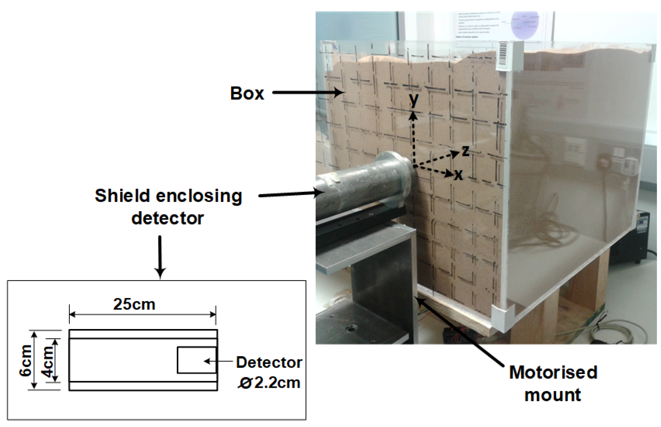
3.1. Gamma Ray Data Acquisition and Processing

The experiment setup for the acquisition of the gamma ray intensity data is as shown in Figure 3. The material volume is represented by a box in which the different materials were placed. The dimension of the box is 40 cm × 50 cm × 40 cm (length × width × height) and it was constructed with acrylic sheets with a thickness of 0.8 cm. Acrylic sheet was used because it is relatively transparent to gamma rays. The front of the box was divided into 4 × 4 cm2 grids in order to identify each measurement position. The gamma ray detector used in the experiment was the CZT/500(s) detector from Ritec (Riga, Latvia). This is a Cadmium Zinc Telluride detector which has a sensing volume of 0.5 cm3 and is sealed in a casing with a diameter of 2.2 cm. Furthermore, the detector was placed inside a hollow cylindrical tungsten shield opened at both ends in order to eliminate background radiation from the laboratory environment.
During the experiment, the box was filled with one of the materials and a 658 kBq Cs-137 radioactive point source was buried at varying depths from 2 cm to 22 cm at 4 cm intervals along the z-axis starting from the origin. This procedure was repeated for each of the materials. At each depth, the pulses from the detector were acquired using an oscilloscope (sampling rate = 500 kSa/s) from the desired number of grids. An acquisition time of 25 min per grid was used throughout the experiment. The acquired pulses were then stored and processed in a personal computer using the pulse height analysis algorithm described in [45] to generate the spectrum of the source at each grid. Therefore, a total of n spectra was acquired per depth where n is the number of grids. In addition, the background spectra for each of the three materials were also measured and subtracted from each of the generated spectrum. Finally, the photo peak function described in [46] was used to extract the number of gamma ray photons (i.e., intensity) at 662 keV from each of the generated spectrum.

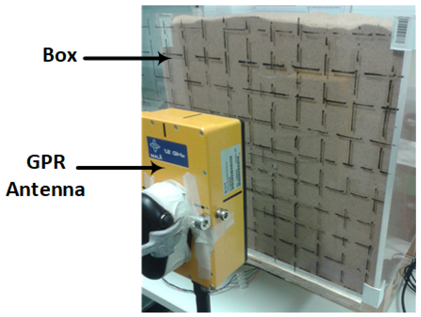
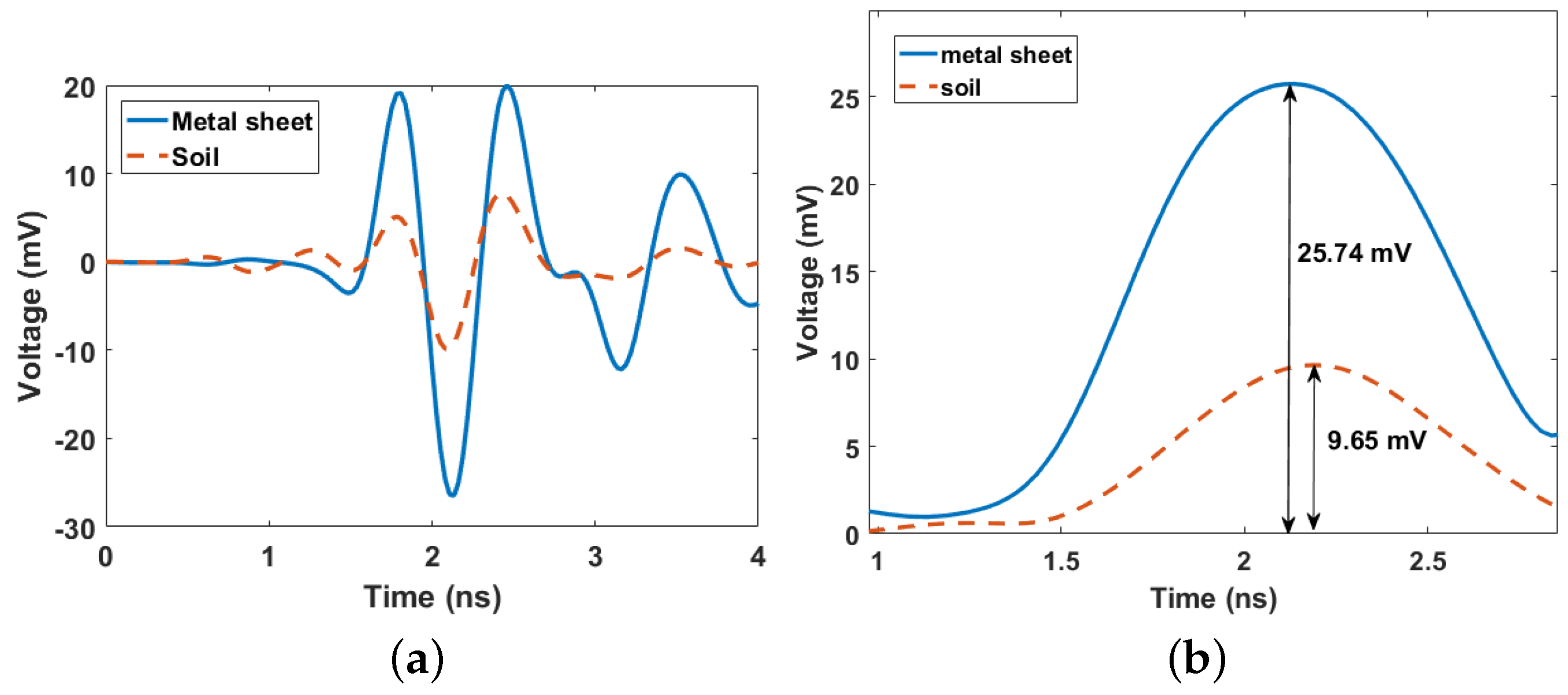
3.2. GPR Data Acquisition and Processing

As mentioned in Subsection 2.3, the first step in bulk density estimation using GPR is the estimation of the bulk permittivity using Equation (4). This will require the measurement of the amplitudes of the reflected pulses from each of the material and that from a metallic surface. The setup for the acquisition of the reflected pulses is shown in Figure 4. The orientation of the setup was kept the same with that of the gamma ray data acquisition to ensure consistency between the data from both experiments. The GPR system used is the MALA CX12 from GuidelineGeo (Sundbyberg, Sweden) with a central frequency of 1.2 GHz. In addition, a sampling frequency of 37 GHz and time window of 8.4 ns was used for throughout the experiment.
During the experiment, the GPR antenna was centrally positioned fifteen centimeters (15 cm) away from the front of the box while the reflected pulse was measured. This was repeated each time the box was filled with a different material. Furthermore, since the bulk permittivity was assumed to be uniform throughout the material volume, all the pulses were measured from this fixed position. In addition, the reflected pulse when the box was empty was also measured and subtracted from the reflected pulses measured when the box was filled with each of the material. This procedure removed the contributions of both the direct wave and box to the measured reflected pulses from the materials. Finally, the reflected pulse from a flat metal sheet was also measured in order to complete the data required to estimate the bulk permittivities of the materials.
After acquisition, the pulses were filtered using a finite impulse response bandpass filter with lower and upper frequencies of 0.5 GHz and 2.5 GHz respectively to remove unwanted frequency components. The filtered pulses from both the soil and metal sheet are shown in Figure 5a. The amplitude values of the pulses were obtained from the peak of the envelope of the Hilbert transform of the pulses. This is also shown in Figure 5b for the pulses from the soil and the metal sheet. Having obtained the required amplitude values, the bulk permittivities of the three materials were then estimated using Equation (4) and are shown in Table 2. The bulk permittivities of both the sand and gravel are consistent with the values reported in [43,47], while that of the soil is higher than both materials because of the water content. Also, note that the bulk permittivity of the gravel is higher than that of the sand despite both materials having approximately the same measured bulk densities. This difference is due to the solid permittivity of gravel which is higher than that of sand. Finally, using the estimated bulk permittivities, the bulk densities of each of the materials were then estimated using the four permittivity mixing formulas i.e., Equations (7)–(11) where the permittivities of water and air were taken to be 80.1 and 1 respectively. These results are presented and discussed in the next section.

4. Results

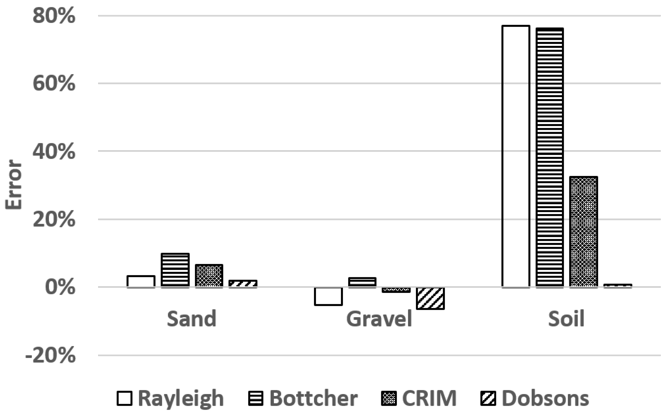
4.1. Bulk Density Estimation

The error in the estimated bulk densities for the four mixing formulas are shown in Figure 6. It can be observed that all the formulas yielded reasonably good estimates for both sand and gravel with an average error of 5% and 3.75%, respectively. However, the Rayleigh and Dobson formulas had the best performance for sand with an error of 3% and 2%, respectively. Conversely, the Bottcher and CRIM formulas had the best performance for the gravel with an error of 3% and −1% (negative errors means that the bulk density was underestimated). However, the significant difference in the performance of the formulas can be observed in the result for soil where all the formulas except the Dobson formula performed very poorly. The overestimation of the bulk density of soil by over 70% by both the Rayleigh and Bottcher formulas can be attributed to the fact that both formulas assume that the mixture is homogeneous [33] which is relatively true for both the sand and gravel samples. Conversely, soil is typically a complex mixture of sand, clay, silt, water, organic matter and other inorganic minerals consequently, the assumption of homogeneity is not valid.
The very good performance of the Dobson formula for soil compared to the poor performance of the CRIM formula is likely due to the inclusion of the effect of bound water by Dobson et al. [37] in their estimation of the value of α in Equation (6). This is because at low water content (as is with the case of the soil used in this study), the water in the soil exists predominantly as bound water [37], i.e., as a thin film around the solid soil particles. Due to their restricted molecular motion, these bound water have a lower permittivity compared to free water in the pore of the soil matrix [35]. Therefore, the assumption that all the water in the soil behaves as free water (see [36]) which is the basis for arriving at a value of 0.5 for α is not correct. However, this assumption can be valid at high water content where the behaviour of free water dominates. This was further confirmed by [32] who observed that an α value of 0.5 seems to be appropriate for fully water-saturated porous media. Finally, since the Dobson formula had the least average error of 4.5% for all materials, its bulk density estimates were used in the subsequent sections to calculate the depth of the buried Cs-137 source.

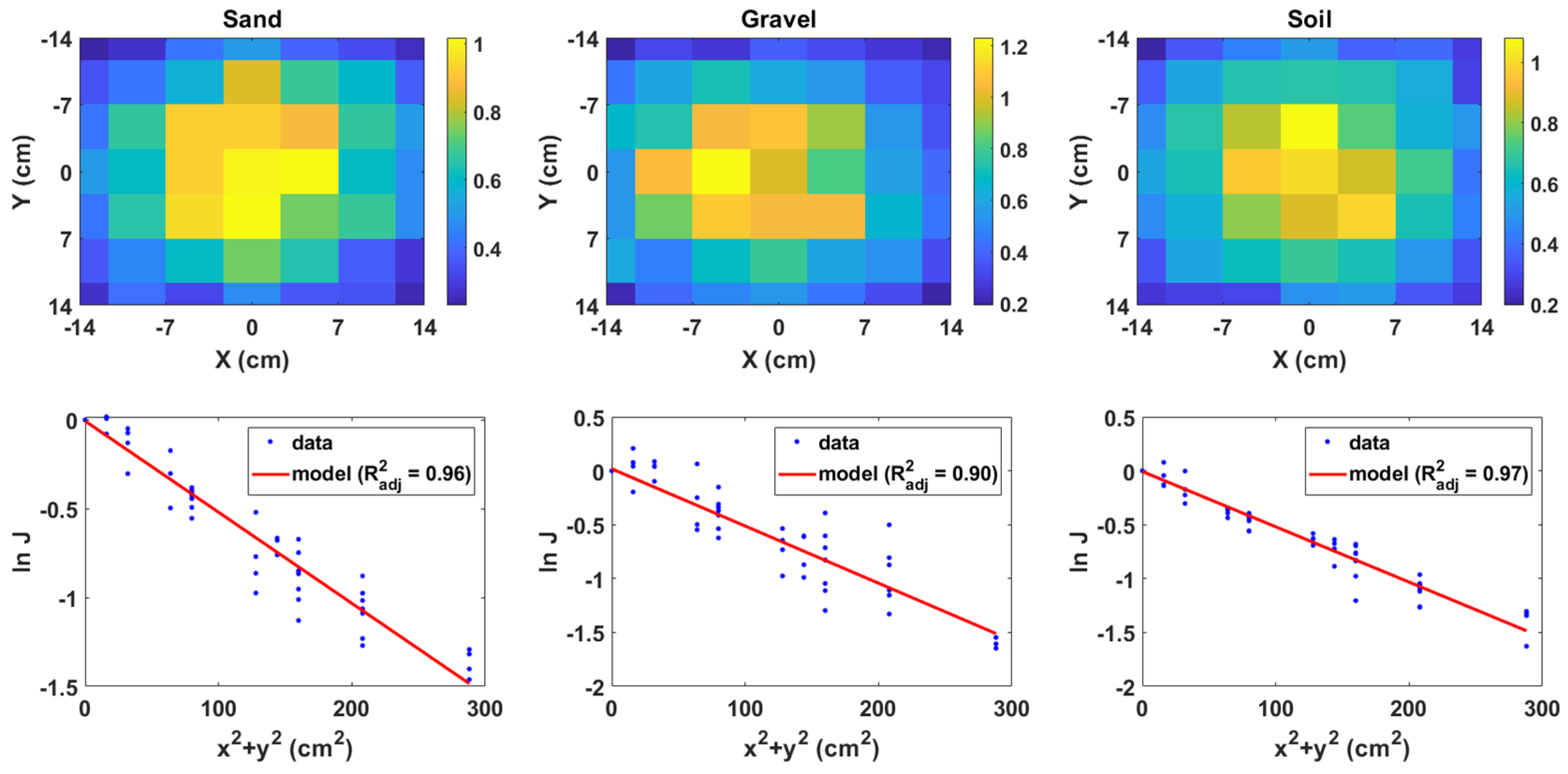
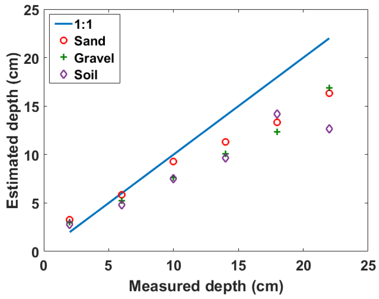
4.2. Depth Estimation of the Buried Cs-137 Radioisotope

The measured gamma ray intensities when the source was buried at 14 cm in the three materials are shown in the top row of Figure 7 as normalised raster images. The intensities were measured from a total of 7 × 7 grids covering a total scan area of 28 × 28 cm2. Furthermore, each pixel value of the image represents the number of gamma ray photons at 662 keV recorded by the detector at that position. The fitting of the attenuation model (i.e., Equation (1)) to the data from each of raster images using the density estimates from the Dobson mixing formula are shown in the corresponding bottom row of Figure 7. A good model fit can be observed for all three materials as indicated by the high adjusted r-squared values.
The estimated depths of the buried Cs-137 radioisotope from the fitted attenuation model are shown in Figure 8 for all three materials. A consistent linear deviation of the estimated depth from the measured depth as the depth increases can be observed in all three materials. This deviation can be attributed to the fact that the attenuation model does not account for the inverse square reduction in the gamma ray intensity as the depth increases. However, a linear correlation between the estimated and measured depths can be visually observed in the figure for all three materials. This means that the measured depth can be predicted from the estimated depth by fitting a linear polynomial to the scatter graph. The fitted linear polynomials for the three materials are given in Table 3. The high adjusted r-squared values is indicative of the good linear correlation between the estimated and measured depths. Finally, it was shown in [45] that the parameters of these linear polynomials (i.e., the gradient and intercept) can be obtained using simulation tools such as MCNPX [48] and then used to correct estimated depths measured from field data.

5. Discussions

The results presented in the previous section has proven the potential of GPR as a tool for estimating the material bulk density required for nonintrusive estimation of the depth of buried radioactive sources. This in situ density estimation will improve the accuracy in determining the depth of penetration of radioactive contaminants in materials such as soil and concrete compared to the use of historical density values. Furthermore, the nonintrusive nature of GPR will ensure that the contaminated material subsurface is not disturbed thereby preventing further spreading of the contamination.
However, one of the potential challenges in applying this depth estimation technique in the field is the time required to move a single gamma detector across the scan area. This can be eliminated by using a square array of gamma detectors since each detector and its shielding covers only a relatively small area of 4 × 4 cm2. The detector array can then be mounted on a trolley to scan the ground surface of the contaminated area. It should also be noted that the 25 min per grid measurement time taken to measure the gamma rays is due to the fact that each signal from the detector was first digitised by an oscilloscope and then transferred to a computer for processing. This time will be substantially reduced by using commercial multichannel analysers. These are dedicated high-speed electronics that process the output from a gamma detector and generate the spectrum of the radioactive source in real-time.
Another difficulty that maybe encountered in the field is the fact that Equation (4) depends only on the change in permittivity at the air-material interface. Consequently, it is unable to measure the vertical variation in the bulk permittivity inside the material which can occur when investigating at greater depths, e.g., up to 1 m. This difficulty can be resolved by iteratively applying Equation (3) to every significant pulse identified in the measure A-scan. This will yield the vertical variation of the permittivity inside the material from which the variation in density can be obtained using the Dobson mixing formula.

6. Conclusions

The use of GPR as a complementary sensor to provide in situ material density data required for the nonintrusive estimation of the depth of buried radioactive sources from radiation data has been demonstrated using three different materials. The results showed that the Dobson permittivity mixing formula provided the best bulk density estimates across the range of materials investigated. Therefore, its results were used with the radiation data to estimated the depth of a buried Cs-137 source using an approximate 3D attenuation model. In addition, different geometries for the measurement of the radiation data were analysed and it was found that measuring along a diagonal pattern can significantly reduce the measurement time and amount of data required to estimate the depth. However, a linear correction factor needs to be applied to the depth estimates to account for deviation of the estimated depth from the measured depth as the depth increases. This limitation will be further investigated in order to make the attenuation model more robust.
Finally, the benefits of combining GPR and radiation detectors are not limited to material density estimation. It also opens the possibility of nonintrusive three dimensional reconstruction of the contaminated subsurface by fusing GPR and radiation images. This will enhance visual monitoring of these type of contaminated environments and provide guidance for autonomous decommissioning systems.

Author Contributions

Conceptualization, I.K.U. and K.A.A.G.; methodology, I.K.U.; validation, I.K.U.; formal analysis, I.K.U.; investigation, I.K.U. and M.D.A.; writing—original draft preparation, I.K.U.; writing—review and editing, I.K.U., K.A.A.G. and M.D.A.; visualization, I.K.U.; supervision, K.A.A.G. and M.D.A.; funding acquisition, K.A.A.G.

Funding

This research was funded by the Engineering and Physical Sciences Research Council, U.K. (EP/N509231/1) and the Nuclear Decommissioning Authority, U.K. The APC was funded by Lancaster University.

Acknowledgments

The authors would like to thank Douglas Offin (National Nuclear Laboratory, UK) for industrial supervision of the project and Richard Wilbraham (Engineering department, Lancaster University, UK) for assistance with the scanning electron microscopy measurements.

Conflicts of Interest

The authors declare no conflict of interest.

References

  1. Laraia, M.T. Nuclear Decommissioning: Planning, Execution and International Experience; Woodhead Publishing Limited: Cambridge, UK, 2012. [Google Scholar]
  2. Sullivan, P.O.; Nokhamzon, J.G.; Cantrel, E. Decontamination and dismantling of radioactive concrete structures. NEA News 2010, 28, 27–29. [Google Scholar]
  3. Popp, A.; Ardouin, C.; Alexander, M.; Blackley, R.; Murray, A. Improvement of a high risk category source buried in the grounds of a hospital in Cambodia. In Proceedings of the 13th International Congress of the International Radiation Protection Association, Glasgow, Scotland, 14–18 May 2012; pp. 1–10. [Google Scholar]
  4. Lal, R.; Fifield, L.; Tims, S.; Wasson, R. 239 Pu fallout across continental Australia: Implications on 239 Pu use as a soil tracer. J. Environ. Radioact. 2017, 178–179, 394–403. [Google Scholar] [CrossRef] [PubMed]
  5. Varley, A.; Tyler, A.; Dowdall, M.; Bondar, Y.; Zabrotski, V. An in situ method for the high resolution mapping of137Cs and estimation of vertical depth penetration in a highly contaminated environment. Sci. Total Environ. 2017, 605–606, 957–966. [Google Scholar] [CrossRef] [PubMed]
  6. Penrose, B.; Johnson née Payne, K.A.; Arkhipov, A.; Maksimenko, A.; Gaschak, S.; Meacham, M.C.; Crout, N.J.; White, P.J.; Beresford, N.A.; Broadley, M.R. Inter-cultivar variation in soil-to-plant transfer of radiocaesium and radiostrontium in Brassica oleracea. J. Environ. Radioact. 2016, 155–156, 112–121. [Google Scholar] [CrossRef] [PubMed]
  7. Adams, J.C.; Mellor, M.; Joyce, M.J. Depth determination of buried caesium-137 and cobalt-60 sources using scatter peak data. IEEE Trans. Nuclear Sci. 2010, 57, 2752–2757. [Google Scholar] [CrossRef]
  8. Shippen, A.; Joyce, M.J. Profiling the depth of caesium-137 contamination in concrete via a relative linear attenuation model. Appl. Radiat. Isotopes 2010, 68, 631–634. [Google Scholar] [CrossRef] [PubMed]
  9. Adams, J.C.; Mellor, M.; Joyce, M.J. Determination of the depth of localized radioactive contamination by 137Cs and 60Co in sand with principal component analysis. Environ. Sci. Technol. 2011, 45, 8262–8267. [Google Scholar] [CrossRef]
  10. Adams, J.C.; Joyce, M.J.; Mellor, M. Depth profiling 137Cs and 60Co non-intrusively for a suite of industrial shielding materials and at depths beyond 50 mm. Appl. Radiat. Isotopes 2012, 70, 1150–1153. [Google Scholar] [CrossRef]
  11. Adams, J.C.; Joyce, M.J.; Mellor, M. The advancement of a technique using principal component analysis for the non-intrusive depth profiling of radioactive contamination. Nuclear Sci. IEEE Trans. 2012, 59, 1448–1452. [Google Scholar] [CrossRef]
  12. Haddad, K.; Al-Masri, M.S.; Doubal, A.W. Determination of 226Ra contamination depth in soil using the multiple photopeaks method. J. Environ. Radioact. 2014, 128, 33–37. [Google Scholar] [CrossRef]
  13. Iwamoto, Y.; Kataoka, J.; Kishimoto, A.; Nishiyama, T.; Taya, T.; Okochi, H.; Ogata, H.; Yamamoto, S. Novel methods for estimating 3D distributions of radioactive isotopes in materials. Nuclear Instrum. Methods Phys. Res. Sect. A Accel. Spectrom. Detect. Assoc. Equip. 2016, 831, 295–300. [Google Scholar] [CrossRef]
  14. Varley, A.; Tyler, A.; Bondar, Y.; Hosseini, A.; Zabrotski, V.; Dowdall, M. Reconstructing the deposition environment and long-term fate of Chernobyl137Cs at the floodplain scale through mobile gamma spectrometry. Environ. Pollut. 2018, 240, 191–199. [Google Scholar] [CrossRef]
  15. Dewey, S.C.; Whetstone, Z.D.; Kearfott, K.J. A method for determining the analytical form of a radionuclide depth distribution using multiple gamma spectrometry measurements. J. Environ. Radioact. 2011, 102, 581–588. [Google Scholar] [CrossRef]
  16. Whetstone, Z.D.; Dewey, S.C.; Kearfott, K.J. Simulation of a method for determining one-dimensional137Cs distribution using multiple gamma spectroscopic measurements with an adjustable cylindrical collimator and center shield. Appl. Radiat. Isotopes 2011, 69, 790–802. [Google Scholar] [CrossRef]
  17. Varley, A.; Tyler, A.; Smith, L.; Dale, P. Development of a neural network approach to characterise 226Ra contamination at legacy sites using gamma-ray spectra taken from boreholes. J. Environ. Radioact. 2015, 140, 130–140. [Google Scholar] [CrossRef] [PubMed]
  18. Varley, A.; Tyler, A.; Smith, L.; Dale, P.; Davies, M. Remediating radium contaminated legacy sites: Advances made through machine learning in routine monitoring of “hot” particles. Sci. Total Environ. 2015, 521–522, 270–279. [Google Scholar] [CrossRef] [PubMed]
  19. Varley, A.; Tyler, A.; Smith, L.; Dale, P.; Davies, M. Mapping the spatial distribution and activity of 226Ra at legacy sites through Machine Learning interpretation of gamma-ray spectrometry data. Sci. Total Environ. 2016, 545–546, 654–661. [Google Scholar] [CrossRef]
  20. Ukaegbu, I.; Gamage, K. A Novel Method for Remote Depth Estimation of Buried Radioactive Contamination. Sensors 2018, 18, 507. [Google Scholar] [CrossRef] [PubMed]
  21. Al-Shammary, A.A.G.; Kouzani, A.Z.; Kaynak, A.; Khoo, S.Y.; Norton, M.; Gates, W. Soil Bulk Density Estimation Methods: A Review. Pedosphere 2018, 28, 581–596. [Google Scholar] [CrossRef]
  22. Tran, A.P.; Andre, F.; Lambot, S. Validation of near-field ground-penetrating radar modeling using full-wave inversion for soil moisture estimation. IEEE Trans. Geosci. Remote Sens. 2014, 52, 5483–5497. [Google Scholar] [CrossRef]
  23. Algeo, J.; Van Dam, R.L.; Slater, L. Early-Time GPR: A Method to Monitor Spatial Variations in Soil Water Content during Irrigation in Clay Soils. Vadose Zone J. 2016, 15. [Google Scholar] [CrossRef] [Green Version]
  24. Koyama, C.N.; Liu, H.; Takahashi, K.; Shimada, M.; Watanabe, M.; Khuut, T.; Sato, M. In-situ measurement of soil permittivity at various depths for the calibration and validation of low-frequency SAR soil moisture models by using GPR. Remote Sens. 2017, 9, 580. [Google Scholar] [CrossRef]
  25. Shamir, O.; Goldshleger, N.; Basson, U.; Reshef, M. Laboratory Measurements of Subsurface Spatial Moisture Content by Ground-Penetrating Radar (GPR) Diffraction and Reflection Imaging of Agricultural Soils. Remote Sens. 2018, 10, 1667. [Google Scholar] [CrossRef]
  26. Al-Qadi, I.L.; Lahouar, S. Measuring layer thicknesses with GPR - Theory to practice. Constr. Build. Mater. 2005, 19, 763–772. [Google Scholar] [CrossRef]
  27. Mahmoudzadeh Ardekani, M.R. Off- and on-ground GPR techniques for field-scale soil moisture mapping. Geoderma 2013, 200–201, 55–66. [Google Scholar] [CrossRef]
  28. Benedetto, A.; Tosti, F.; Ortuani, B.; Giudici, M.; Mele, M. Soil moisture mapping using GPR for pavement applications. In Proceedings of the 7th International Workshop on Advanced Ground Penetrating Radar, Nantes, France, 2–5 July 2013; pp. 1–5. [Google Scholar] [CrossRef]
  29. Loizos, A.; Plati, C. Accuracy of pavement thicknesses estimation using different ground penetrating radar analysis approaches. NDT E Int. 2007, 40, 147–157. [Google Scholar] [CrossRef]
  30. Leng, Z.; Al-Qadi, I.L.; Lahouar, S. Development and validation for in situ asphalt mixture density prediction models. NDT E Int. 2011, 44, 369–375. [Google Scholar] [CrossRef]
  31. Shangguan, P.; Al-Qadi, I.L.; Lahouar, S. Pattern recognition algorithms for density estimation of asphalt pavement during compaction: A simulation study. J. Appl. Geophys. 2014, 107, 8–15. [Google Scholar] [CrossRef]
  32. Brovelli, A.; Cassiani, G. Effective permittivity of porous media: A critical analysis of the complex refractive index model. Geophys. Prospect. 2008, 56, 715–727. [Google Scholar] [CrossRef]
  33. Sihvola, A.H. Self-Consistency Aspects of Dielectric Mixing Theories. IEEE Trans. Geosci. Remote Sens. 1989, 27, 403–415. [Google Scholar] [CrossRef]
  34. Birchak, J.R.; Gardner, C.G.; Hipp, J.E.; Victor, J.M. High Dielectric Constant Microwave Probes for Sensing Soil Moisture. Proc. IEEE 1974, 62, 93–98. [Google Scholar] [CrossRef]
  35. Roth, K.; Schulin, R.; Hler, H.F.L.; Attinger, W. Calibration of Time Domain Reflectometry for Water Content Measurement. Water Resour. 1990, 26, 2267–2273. [Google Scholar]
  36. Gardner, C.M.; Dean, T.J.; Cooper, J.D. Soil water content measurement with a high-frequency capacitance sensor. J. Agric. Eng. Res. 1998, 71, 395–403. [Google Scholar] [CrossRef]
  37. Dobson, M.C.; Ulaby, F.T.; Hallikainen, M.T.; El-Rayes, M.D.A. Microwave Dielectric Behavior of Wet Soil-Part II: Dielectric Mixing Models. IEEE Trans. Geosci. Remote Sens. 1985, GE-23, 35–46. [Google Scholar] [CrossRef]
  38. Peplinski, N.R.; Ulaby, F.T.; Dobson, M.C. Dielectric Properties of Soils in the 0.3–1.3-GHz Range. IEEE Trans. Geosci. Remote Sens. 1995, 33, 803–807. [Google Scholar] [CrossRef]
  39. Rayleigh, L. LVI. On the influence of obstacles arranged in rectangular order upon the properties of a medium. Lond. Edinb. Dublin Philos. Mag. J. Sci. 1892, 34, 481–502. [Google Scholar] [CrossRef]
  40. Bottcher, C.J.F.; Borderwijk, P. Theory of Electric Polarization I1; Elsevier: Amsterdam, The Netherlands, 1978. [Google Scholar]
  41. McConn, R.; Gesh, C.J.; Pagh, R.; Rucker, R.A.; Williams, R. Compendium of Material Composition Data for Radiation Transport Modelling; Technical Report; Pacific Northwest National Laboratory: Washington, DC, USA, 2011. [Google Scholar]
  42. National Institute of Standards and Technology. X-ray Mass Attenuation Coefficients; National Institute of Standards and Technology: Gaithersburg, MD, USA, 2004. [Google Scholar]
  43. Tosti, F.; Bianchini Ciampoli, L.; Calvi, A.; Alani, A.M.; Benedetto, A. An investigation into the railway ballast dielectric properties using different GPR antennas and frequency systems. NDT E Int. 2018, 93, 131–140. [Google Scholar] [CrossRef]
  44. Schjønning, P.; McBride, R.; Keller, T.; Obour, P. Predicting soil particle density from clay and soil organic matter contents. Geoderma 2017, 286, 83–87. [Google Scholar] [CrossRef]
  45. Ukaegbu, I.; Gamage, K. A Model for Remote Depth Estimation of Buried Radioactive Wastes Using CdZnTe Detector. Sensors 2018, 18, 1612. [Google Scholar] [CrossRef] [PubMed]
  46. Mortreau, P.; Berndt, R. Characterisation of cadmium zinc telluride detector spectra—Application to the analysis of spent fuel spectra. Nuclear Instrum. Methods Phys. Res. Sect. A Accel. Spectrometers Detect. Assoc. Equip. 2001, 458, 183–188. [Google Scholar] [CrossRef]
  47. Mätzler, C. Microwave Permittivity of Dry Sand. IEEE Trans. Geosci. Remote Sens. 1998, 36, 317–319. [Google Scholar] [CrossRef]
  48. Pelowitz, D.B. MCNPX User’s Manual: Version 2.7.0; Los Alamos National Laboratory: Los Alamos, NM, USA, 2011. [Google Scholar]
Figure 1. Radioactive point source S buried in a material volume.
Remotesensing 11 00141 g001
Figure 2. Principles of ground penetrating radar (GPR). Reflected waves from boundaries a recorded by the receiver and displayed as a time varying signal called an A-scan.
Remotesensing 11 00141 g002
Figure 3. Setup for the gamma ray measurements. The Cs-137 point source was placed at varying position along the z-axis using a pipe that protruded behind the box, while the intensity was measured at the desired positions on the surface of the box.
Remotesensing 11 00141 g003
Figure 4. Setup for the GPR reflected pulse measurements. The antenna was placed 15 cm from the surface of the box.
Remotesensing 11 00141 g004
Figure 5. (a) Measured reflected pulses from the air-soil and air-metal interfaces without time-offset correction. Both pulses can be seen to arrive between 1.4–2.6 ns; (b) Envelope of the Hilbert transform of both pulses.
Remotesensing 11 00141 g005
Figure 6. Error in the estimated bulk densities of the three materials under investigation.
Remotesensing 11 00141 g006
Figure 7. Normalised raster images of the Cs-137 source buried at a depth of 14 cm for each of the material (top row). Corresponding fit of the attenuation model for each of the depth images (bottom row).
Remotesensing 11 00141 g007
Figure 8. Estimated depths of the buried Cs-137 source for the three materials.
Remotesensing 11 00141 g008
Table 1. Properties of the materials used in the study.
Sand10 mm GravelSoil
Bulk density ( ρ b ) (g cm−3)1.521.541.26
Mass attenuation coefficient ( μ m ) at 662 keV0.07760.07750.0773
Solid permittivity ( ϵ s )4.76.54.7
Specific density ( ρ s ) (g cm−3)2.652.652.65
Water content ( θ ) (%)0.00.06.0
Table 2. Estimated bulk permittivity for the three materials using Equation (4).
SandGravelSoil
Bulk permittivity ( ϵ b )2.933.574.84
Table 3. Linear polynomials fitted to the scatter graph of Figure 8 where z e s t is the estimated depth and z m e a is the measured depth. This can be used as calibration equations to correct for the deviation of the estimated depth from the measured depth.
Material y = ax + b ± error R adj 2
Sand z e s t = 0.64 z m e a + 2.2 ± 1.1 0.99
Gravel z e s t = 0.63 z m e a + 1.9 ± 1.2 0.99
Soil z e s t = 0.59 z m e a + 1.5 ± 1.9 0.95

