Efficient Lidar Signal Denoising Algorithm Using Variational Mode Decomposition Combined with a Whale Optimization Algorithm

Abstract

Although lidar is a powerful active remote sensing technology, lidar echo signals are easily contaminated by noise, particularly in strong background light, which severely affects the retrieval accuracy and the effective detection range of the lidar system. In this study, a coupled variational mode decomposition (VMD) and whale optimization algorithm (WOA) for noise reduction in lidar signals is proposed and demonstrated completely. The combination of optimal VMD parameters of decomposition mode number K and quadratic penalty α was obtained by using the WOA and was critical in acquiring satisfactory analysis results for VMD denoising technology. Then, the Bhattacharyya distance was applied to identify the relevant modes, which were reconstructed to achieve noise filtering. Simulation results show that the performance of the proposed VMD-WOA method is superior to that of wavelet transform, empirical mode decomposition, and its variations. Experimentally, this method was successfully used to filter a lidar echo signal. The signal-to-noise ratio of the denoised signal was increased to 23.92 dB, and the detection range was extended from 6 to 10 km.

1. Introduction

Lidar is a combination of traditional radar technology and modern laser technology and has the advantages of high resolution, wide detection range, and strong anti-interference ability [1]. Its applications in atmospheric remote sensing detection, e.g., aerosol, cloud layer, and visibility, have become increasingly important [2,3]. However, the power of the lidar echo signal decays with the exponential attenuation of the aerosol extinction coefficient and the square of the distance between the lidar and the target according to the lidar equation, and the signal can be easily interfered with by noise from electric fluctuations and stray lights [4]. Moreover, the lidar echo signal is susceptible to strong background sunlight noise, dark current noise, and thermal noise [5]. Useful signals are inevitably contaminated by noise, which will directly affect the effective working range and the detection precision. Therefore, the lidar backscattering signal must be effectively denoised.

In the last few decades, several filtering methods based on nonlinear and nonstationary signal processing, such as Kalman filtering (KF), wavelet transform (WT), and empirical mode decomposition (EMD), have been proposed to denoise lidar signals. KF can be defined as a recursive estimation algorithm with minimum mean square error as the best criterion; however, this method will lose accuracy when the aerosol extinction coefficient changes sharply [6,7]. WT can decompose the signal into different frequencies through multiscale analysis and has good time–frequency localization characteristics. However, WT is hampered by the problems of selecting suitable wavelet basis functions and the decomposition level [4,8]. EMD technology makes up for the limitations of WT and KF and has good adaptability, thereby enabling it to efficiently reflect the local frequency characteristics of the signal [9]. Nevertheless, EMD and its variants still have some drawbacks, such as mode mixing and end effects [10].

Variational mode decomposition (VMD), proposed by Dragomiretskiy and Zosso in 2014, is a new adaptive signal decomposition method that has a different process of mode decomposition compared with EMD [11]. It has obvious advantages in dealing with nonrecursive signals, which can not only overcome the mode mixing problems in EMD but also obtain a better filtering effect by using its own Wiener filtering characteristics. VMD has been successfully implemented in many fields, such as mechanical diagnosis, biomedical sciences, and hydropower unit vibration signal processing [12,13,14]. Despite VMD’s contributions, two crucial parameters need to be resolved: the decomposition mode number K and the quadratic penalty α [15]. These two parameters are usually selected in a certain range. If they are obtained by the trial-and-error method, it will require tens of thousands of operations and will waste a lot of time. For this reason, the parameter values are usually determined based on experience and convenience, which greatly limits the performance of the VMD method and may cause inaccurate decomposition results. Therefore, appropriate methods are needed to obtain the optimal values of these two parameters, and various algorithms have been proposed. Li et al. proposed an independence-oriented VMD method, which finds the most suitable mode number by peak searching and the similarity principle; however, this method does not consider the influence of the bandwidth control parameter on decomposition results [16]. Shi et al. investigated a precise feature extraction method that optimizes the two parameters K and α for VMD independently [17]. However, they neglected the interaction between the two parameters [18,19]. Selecting relevant modes is also an important issue. At present, the indicators for selecting relevant modalities are correlation coefficient, permutation entropy, approximate entropy, and Hausdorff distance, among others [14,18,19,20].

In this paper, a VMD method combined with the whale optimization algorithm (WOA) is presented and used to reduce signal interference from background light and electric noises for a lidar echo signal. The proposed method utilizes the WOA to obtain the optimal parameter combination of decomposition mode number K and quadratic penalty α. The signal is reconstructed by using the relevant modes, which are selected by calculating the Bhattacharyya distance between the probability density function (PDF) of each mode and the input signal. Four synthetic signals are applied to validate the feasibility of the VMD-WOA model. Numerical exploration shows that the new method can achieve improved results in terms of accuracy and signal-to-noise ratio (SNR) than the method presented in our previous work [21] and other technologies.

2. Brief Description of the VMD Algorithm

The VMD algorithm can decompose any signal into an ensemble of band-limited intrinsic mode functions (BLIMFs) [22]. To evaluate the bandwidth of each mode, VMD is represented as a constrained variational problem, which is given as follows:

$$\begin{array}{l}\underset{\left\{u_k\right\},\left\{{\omega }_k\right\}}{\min }\left\{{\displaystyle \sum _{k=1}^K{\Vert {\partial }_t[(\delta \left(t\right)+\frac{j}{\pi t})\times u_k\left(t\right)]e^{-j{\omega }_{k}t}\Vert }_2^2}\right\}\\ s.t.{\displaystyle \sum _{k=1}^K{u}_k=f}\end{array},$$

(1)

where u_k is the kth mode, ω_k is the center frequency, ${\partial }_t$ represents the gradient with respect to t, t is the time script, δ(t) denotes the impulse function, ‖…‖₂ is the norm, ${\Vert {\partial }_t[(\delta \left(t\right)+\frac{j}{\pi t})\times u_k\left(t\right)]e^{-j{\omega }_{k}t}\Vert }_2^2$ represents the bandwidth of each mode, and f is the original signal to be decomposed.

Taking the quadratic penalty α and Lagrangian multiplier λ into consideration, we can convert the above constrained problem into the unconstrained variational problem. The augmented Lagrangian is expressed as follows:

$$L\left(\left\{u_k\right\},\left\{{\omega }_k\right\},\lambda \right)=\alpha {\displaystyle \sum _k{\Vert {\partial }_t[(\delta \left(t\right)+\frac{j}{\pi t})\times u_k\left(t\right)]e^{-j{\omega }_{k}t}\Vert }_2^2}+{\Vert f(t)-{\displaystyle \sum _k{u}_k\left(t\right)}\Vert }_2^2+\langle \lambda \left(t\right),f\left(t\right)-{\displaystyle \sum _k{u}_k\left(t\right)}\rangle .$$

(2)

The solution to the original minimization problem of Equation (1) is the saddle point of the augmented Lagrangian L in a sequence of iterative sub-optimizations called the alternate direction method of multipliers (ADMM). The formula is given as

$$u_k^{n+1}=\underset{u_k\in X}{\arg \min }\left\{\alpha {\Vert {\partial }_t[(\delta \left(t\right)+\frac{j}{\pi t})\times u_k\left(t\right)]e^{-j{\omega }_{k}t}\Vert }_2^2+{\Vert f(t)-{\displaystyle \sum _i{u}_i\left(t\right)+\frac{\lambda \left(t\right)}{2}}\Vert }_2^2\right\}.$$

(3)

According to the ADMM optimization approach, updating u_k and ω_k in two directions is assumed to help realize the analysis process of VMD, and the solutions for them are as follows:

$${\widehat{u}}_k^{n+1}\left(\omega \right)=\frac{\widehat{f}\left(\omega \right)-{\displaystyle {\sum }_{i\ne k}{\widehat{u}}_i\left(\omega \right)+\frac{\widehat{\lambda }\left(\omega \right)}{2}}}{1+2\alpha {\left(\omega -{\omega }_k\right)}^2},$$

(4)

$${\omega }_k^{n+1}=\frac{{\displaystyle {\int }_0^{\infty }\omega {\left|{\widehat{u}}_k(\omega )\right|}^{2}d\omega }}{{\displaystyle {\int }_0^{\infty }{\left|{\widehat{u}}_k(\omega )\right|}^{2}d\omega }}.$$

(5)

For efficient signal reconstruction, the Lagrangian multiplier is also updated using the following equation:

$${\widehat{\lambda }}^{n+1}\left(\omega \right)={\widehat{\lambda }}^n\left(\omega \right)+\tau \left(\widehat{f}\left(\omega \right)-{\displaystyle {\sum }_k{\widehat{u}}_k^{n+1}}\left(\omega \right)\right).$$

(6)

The algorithm repeats the iterative process according to Equations (4)–(6) until the convergence stop condition is satisfied. The stop condition is given by

$${{\displaystyle {\sum }_k\Vert {\widehat{u}}_k^{n+1}-{\widehat{u}}_k^n\Vert }}_2^2/\Vert {\widehat{u}}_k^n\Vert <e,$$

(7)

where ${\widehat{u}}_k$ is the spectrum of the mode, $\widehat{f}\left(\omega \right)$ is the spectrum of the signal, τ is the noise tolerance, and n is the iteration number. The pseudocode of VMD is summarized in Algorithm 1.

Algorithm 1. Pseudocode for VMD

1: Initialize ${\widehat{u}}_k,{\omega }_k\to 0$

2: Update ${\widehat{u}}_k$ $\to$ ${\widehat{u}}_k^{n+1}\left(\omega \right)=\frac{\widehat{f}\left(\omega \right)-{\displaystyle {\sum }_{i\ne k}{\widehat{u}}_i\left(\omega \right)+\frac{\widehat{\lambda }\left(\omega \right)}{2}}}{1+2\alpha {\left(\omega -{\omega }_k\right)}^2}$

3: Update ${\omega }_k$ $\to$ ${\omega }_k^{n+1}=\frac{{\displaystyle {\int }_0^{\infty }\omega {\left|{\widehat{u}}_k(\omega )\right|}^{2}d\omega }}{{\displaystyle {\int }_0^{\infty }{\left|{\widehat{u}}_k(\omega )\right|}^{2}d\omega }}$

4: Update ${\widehat{\lambda }}^n$ $\to$ ${\widehat{\lambda }}^{n+1}\left(\omega \right)={\widehat{\lambda }}^n\left(\omega \right)+\tau \left(\widehat{f}\left(\omega \right)-{\displaystyle {\sum }_k{\widehat{u}}_k^{n+1}}\left(\omega \right)\right)$ until convergence ${{\displaystyle {\sum }_k\Vert {\widehat{u}}_k^{n+1}-{\widehat{u}}_k^n\Vert }}_2^2/\Vert {\widehat{u}}_k^n\Vert <e$.

3. Principle of the VMD-WOA Model for Noise Reduction

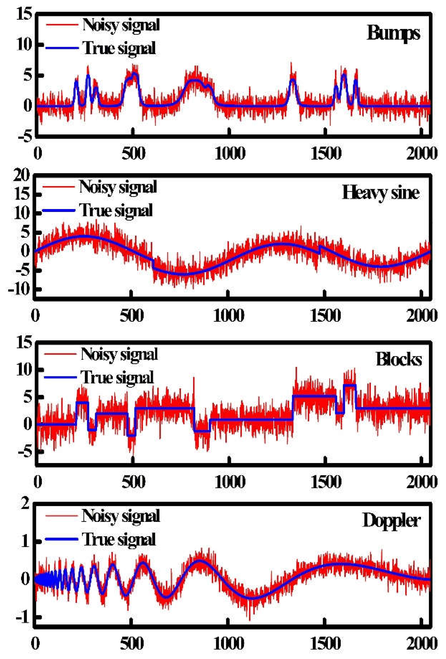
3.1. Optimization of VMD Parameters Based on the WOA

The WOA, first proposed by Mirjalini and Lewis in 2016, is an efficient search and optimization algorithm that was inspired by the bubble-net attacking strategy of whales [23]. When humpback whales obtain the location of prey, they dive deeply, create bubbles in a spiral shape around the prey, and swim to the surface to attack the prey during the maneuver. The mathematical model of the WOA is mainly divided into three phases: encircling the prey, establishing spiral bubbles, and searching for the prey. This novel method requires minimal parameter adjustments and has fast convergence speed and strong global search ability [24]. When using the WOA to determine the key parameters of VMD, the specific operation steps are as follows:

(i) Encircling the prey

In the WOA, a candidate solution is considered the prey position. The encirclement of the humpback whales around the prey can be formulated by the following formulas:

$$\overrightarrow{D}=\left|\overrightarrow{C}\cdot \overrightarrow{X_i^{*}}-\overrightarrow{X_i}\right|,$$

(8)

$$\overrightarrow{X_{i+1}}=\overrightarrow{X_i^{*}}-\overrightarrow{A}\cdot \overrightarrow{D},$$

(9)

where $\overrightarrow{X}$ is the whales’ position vector, $\overrightarrow{X^{\ast }}$ denotes the prey position vector of the best solution obtained, and i represents the current iteration. $\overrightarrow{A}$ and $\overrightarrow{C}$ are coefficient vectors, which can be calculated as follows:

$$\overrightarrow{A}=2\overrightarrow{a}\cdot \overrightarrow{r}-\overrightarrow{a},$$

(10)

$$\overrightarrow{C}=2\cdot \overrightarrow{r},$$

(11)

where vector a is linearly decreased from 2 to 0 over the process of iteration and the random vector r lies in (0, 1).

(ii) Establishing spiral bubbles

There are two existing approaches to the bubble-net behavior of the whales, namely, the shrinking encircling mechanism and the spiral updating position. To model the two behaviors simultaneously, the assumption is that a 50% probability exists in choosing either the shrinking encircling mechanism or the spiral model to update the positions of the whales during optimization. The mathematical model is as follows:

$$\overrightarrow{X_{i+1}}=\{\begin{array}{cc}\overrightarrow{X_i^{*}}-\overrightarrow{A}\cdot \overrightarrow{D}& p<0.5\\ \overrightarrow{D^{\prime }}\cdot e^{bl}\cdot \cos \left(2\pi l\right)+\overrightarrow{X_i^{*}}& p\ge 0.5\end{array},$$

(12)

where $\overrightarrow{D^{\prime }}=\left|\overrightarrow{X_i^{*}}-\overrightarrow{X_i}\right|$ indicates the distance of the current whale to the prey (best solution obtained so far), b is a constant for determining the shape of the logarithmic spiral, l is a random number in the range of −1 to 1, and p is the probability number in (0, 1).

(iii) Searching for the prey

In addition to employing the bubble-net search strategy, humpback whales also randomly search for prey. If |A| ≥ 1, then the position of a search agent will be updated according to a randomly chosen search agent X_rand. The mathematical model is as follows:

$$\overrightarrow{D}=\left|\overrightarrow{C}\cdot \overrightarrow{X_{rand}}-\overrightarrow{X}\right|,$$

(13)

$$\overrightarrow{X_i}=\overrightarrow{X_{rand}}-\overrightarrow{A}\cdot \overrightarrow{D}.$$

(14)

To achieve parameter optimization through the WOA, the fitness function needs to be determined. Energy entropy is used to characterize the distribution of signal energy [25]. A small energy entropy corresponds to increased significance of the corresponding signal in the total energy. The energy entropy values of each mode are calculated by using the VMD model under the positions of the search agents according to the following formula:

$$H=-{\displaystyle \sum _{k=1}^{K}p\left(k\right)}logp\left(k\right),$$

(15)

where p(k) = E_k/E is the percentage of the energy of the kth mode in the total signal energy, $E_k={\displaystyle \sum _t{u}_k{(t)}^2}$, and $E={\displaystyle \sum _k{E}_k}$.

The lowest energy entropy value is called the local minimum energy entropy value and is used as the fitness function in the optimization process [15,26]. It can be described as follows:

$$fitness=\underset{\gamma =\left(K,\alpha \right)}{\min }\left\{{\min }_L{H}_{imf}\right\}.$$

(16)

The pseudocode for the parameter optimization of VMD based on the WOA is presented in Algorithm 2. The WOA algorithm starts with a set of random solutions. At each iteration, the search agents update their positions with respect to either a randomly chosen search agent or the best solution obtained so far. The parameter a is decreased from 2 to 0 in order to provide exploration and exploitation, respectively. A random search agent is chosen when |A| ≥ 1, while the best solution is selected when |A| < 1 for updating the position of the search agents. Depending on the value of p, the WOA is able to switch between spiral and circular movements. Finally, the optimization process is completed when the termination criterion is satisficed and the parameters of K and α can be obtained in X*.

Algorithm 2. Pseudocode for WOA

Initialize the whale population position X

Calculate the fitness of each search agent

X* is the best search agent while (i < maximum iteration number)   for each search agent   Update a, A, C, l, and p    if1 (p < 0.5)     if2 (|A| < 1)      Update the position of the current search agent by the Equation (9)     else if2 (|A| ≥ 1)      Select a random search agent (Xrand)      Update the position of the current search agent by the Equation (14)     end if2    else if1 (p ≥ 0.5)     Update the position of the current search by the Equation (12)    end if1

end for   Check if any search agent goes beyond the search space and amend it   Calculate the fitness of each search agent   Update X* if there is a better solution   i = i + 1 end while return X*

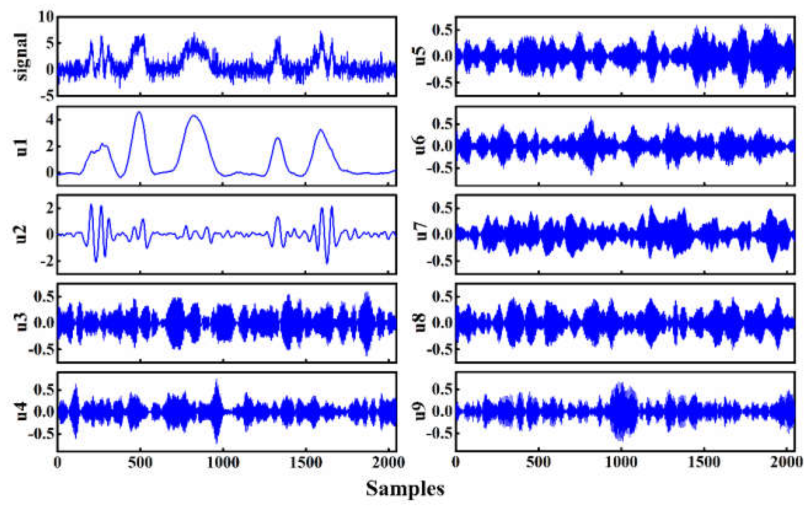
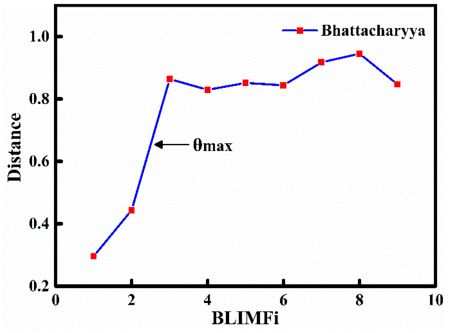
3.2. Identification of Relevant Modes

A probability density function (PDF) can reflect the difference between the distribution of signals [27]. Thus, we use the kernel smoothing density function to estimate the PDFs of each mode and the input signal. The relevant and irrelevant modes are distinguished by calculating their similarity. The similarity measure of input signal f and each mode BLIMF_i, C(i), is defined as follows:

$$C\left(i\right)=distance\left[pdf\left(f\right),pdf\left(BLIM{F}_i\right)\right].$$

(17)

Here, the Bhattacharyya distance is used to measure the distance of two PDFs, which is an effective approach to prove similarity. For probability distributions P and Q over the same domain F, the Bhattacharyya distance is defined as:

$$D_B\left(P,Q\right)=-ln\left(BC\left(P,Q\right)\right).$$

(18)

For discrete probability distributions,

$$BC\left(P,Q\right)={\displaystyle \sum _{f\in F}\sqrt{P\left(f\right)Q\left(f\right)}}.$$

(19)

For continuous probability distributions,

$$BC\left(P,Q\right)={\displaystyle \int \sqrt{P\left(f\right)Q\left(f\right)}df}.$$

(20)

Relevant modes can be determined by evaluating the slope of two adjacent PDFs’ distance between the mode and the input signal [21]. The maximum slope θ can be defined as:

$$\begin{array}{cc}\theta =max\left|C\left(i+1\right)-C\left(i\right)\right|& i=1,2,\dots ,\left(N-1\right)\end{array}.$$

(21)

The demarcation index of relevant and irrelevant modes is as follows:

K_r = i.

(22)

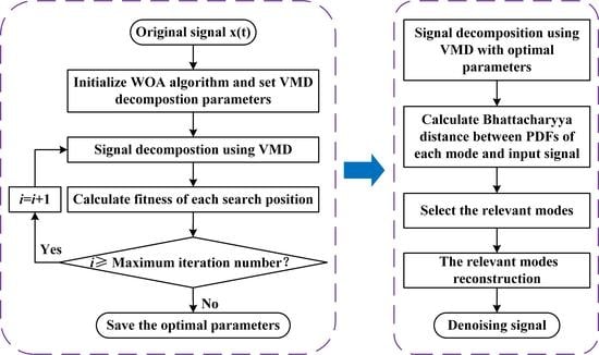
3.3. Proposed VMD-WOA Methodology

Figure 1 shows the flowchart of the VMD-WOA algorithm. The detailed steps of this algorithm are as follows:

Step 1: The original signal f is input. The ranges of the VMD parameters to be optimized are set and the WOA model is initialized, including the number of search agents and the maximum iteration number. Here, K takes an integer in the interval (2,15), α is assigned in the interval (1000–10,000), the number of search agents is 30, and the maximum number of iterations is 15.

Step 2: The signal is decomposed by using VMD. The fitness of each search position is calculated. The minimum fitness value for each iteration is saved.

Step 3: The loop is iterated until the maximum iteration number is reached, i.e., whether i ≥ maximum iteration number. If yes, end the iteration. Otherwise, let i = i + 1 and continue the iteration, saving the optimal parameters and the best fitness value.

Step 4: The signal is decomposed by VMD with optimal parameters.

Step 5: The Bhattacharyya distance between the PDF of each mode and the input signal is calculated.

Step 6: The relevant modes are selected and reconstructed to denoise the signal.

4. Results and Discussion

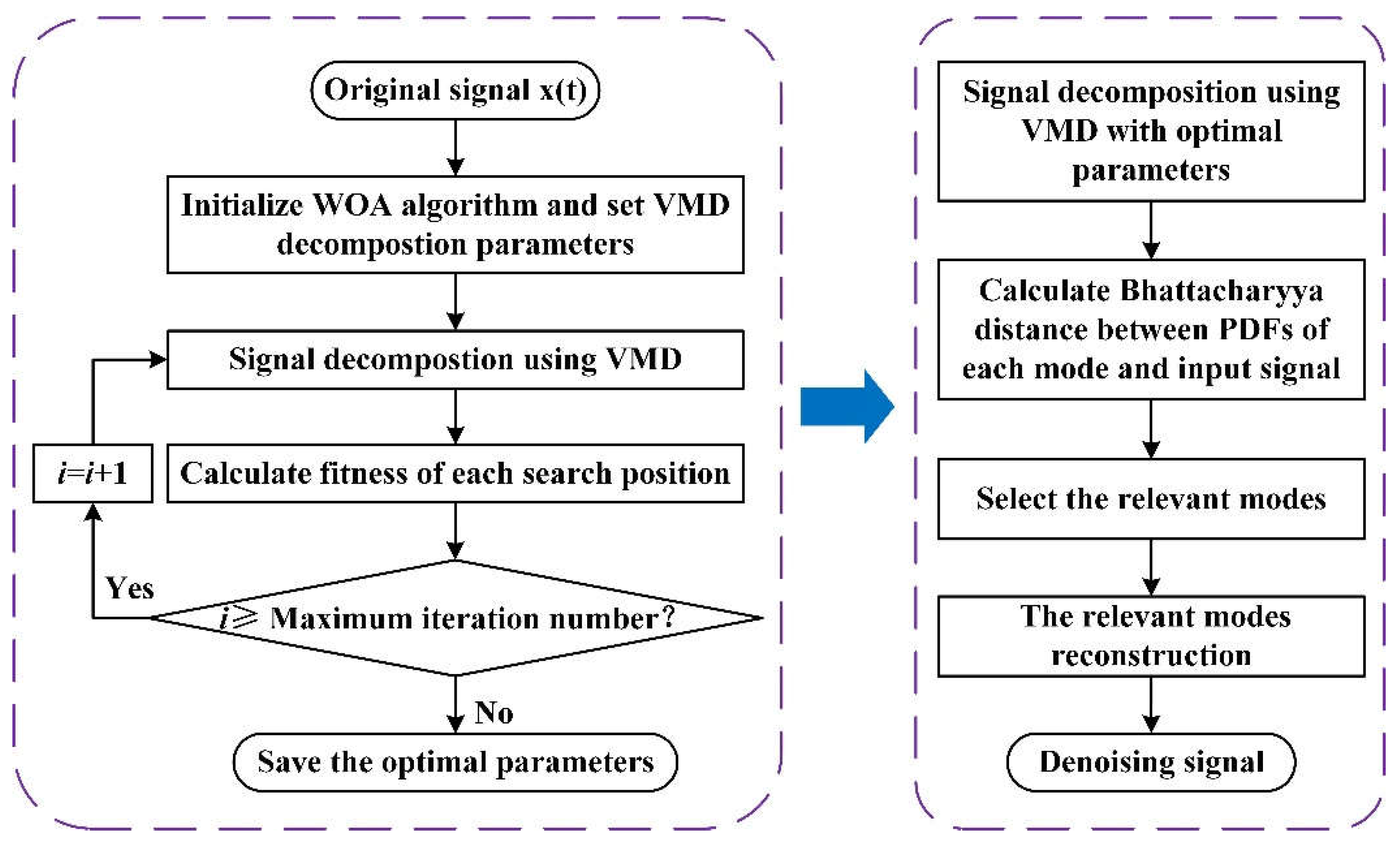
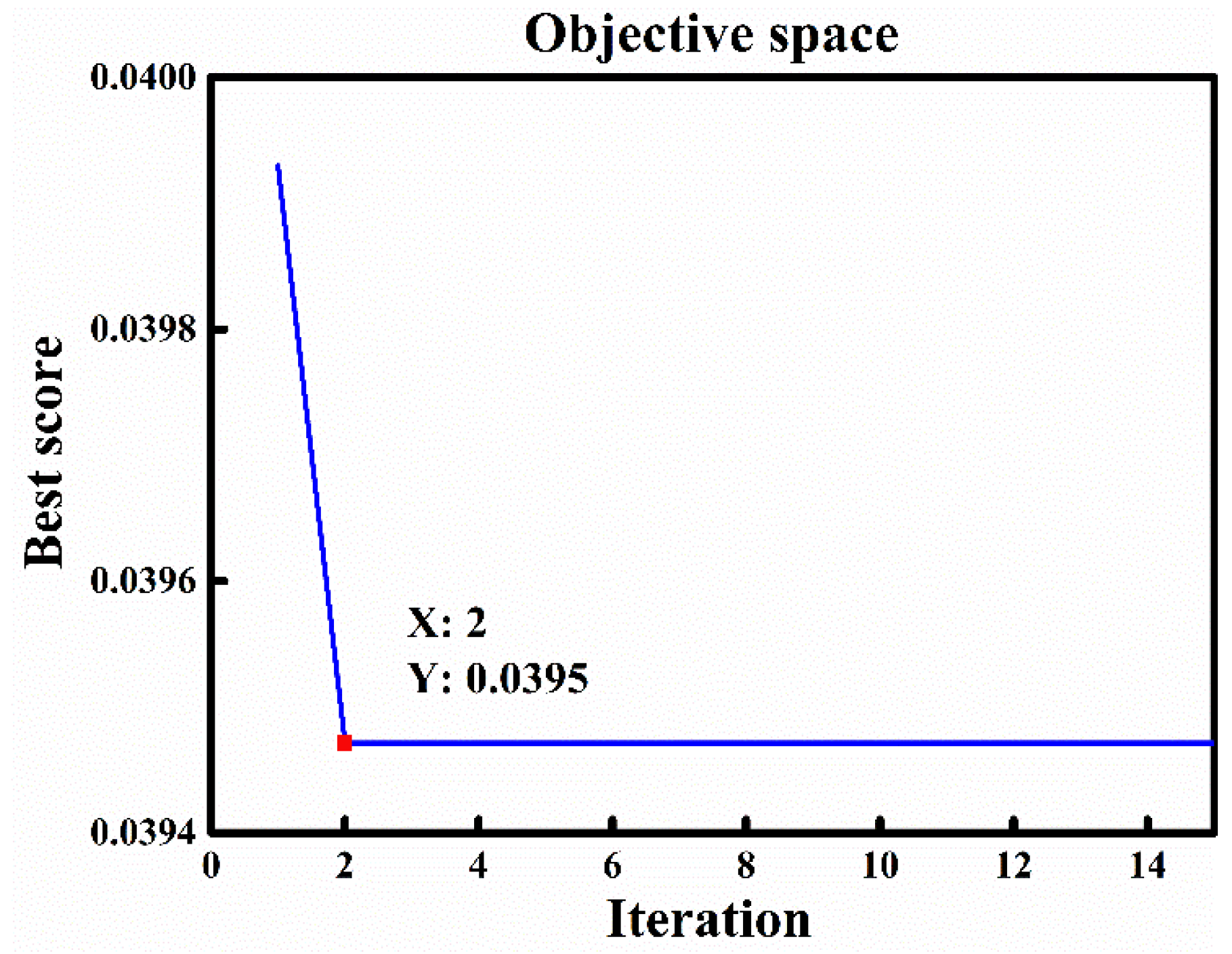
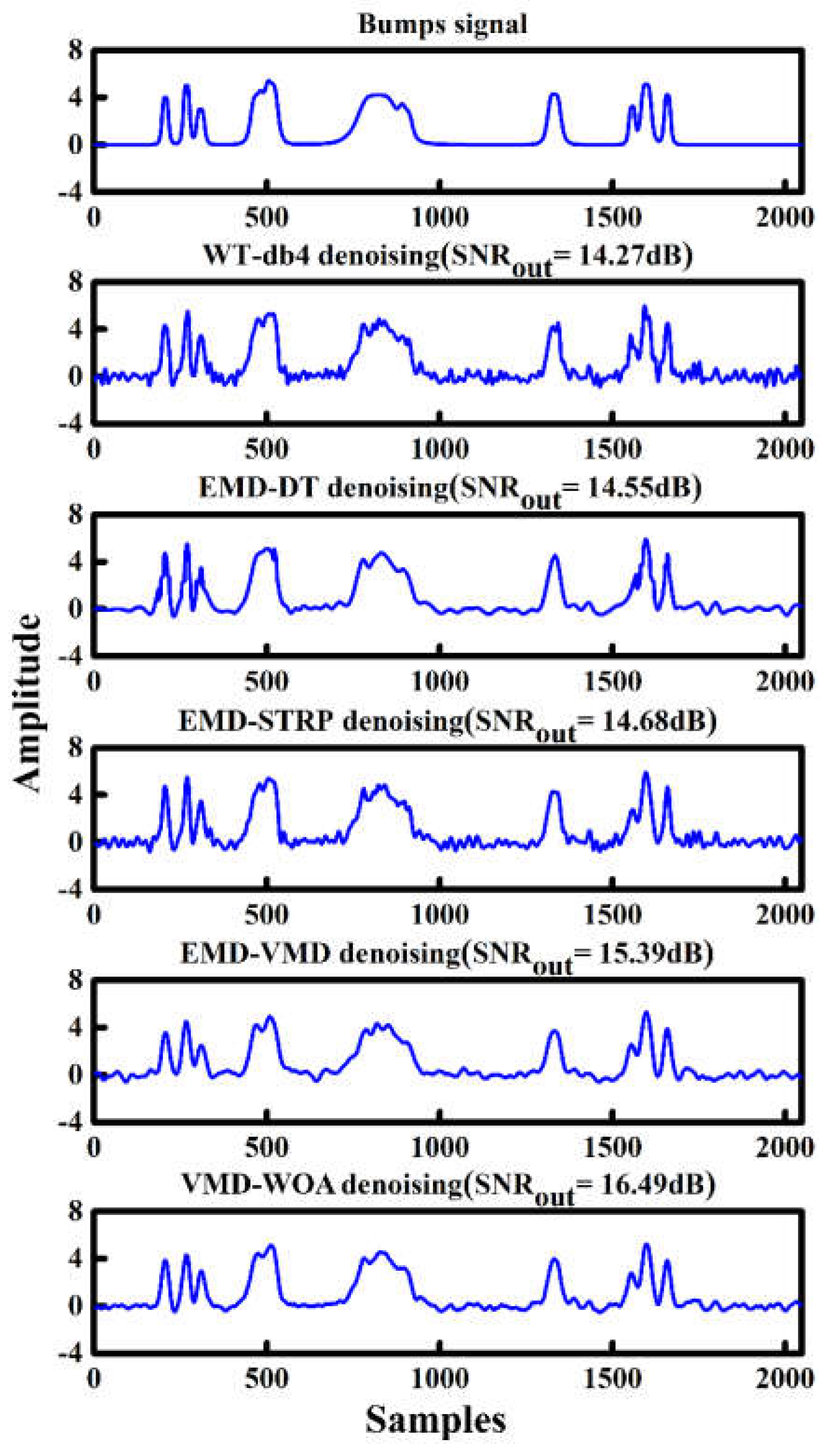
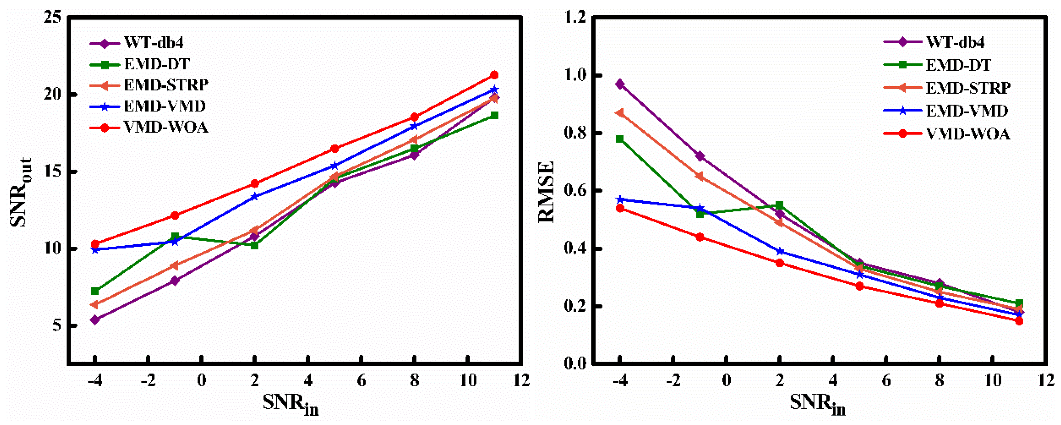
4.1. Experiments with Simulated Signals

To test the effectiveness of the proposed method, preliminary simulations were conducted to reduce the noise in simulated signals. The synthetic signals, namely, Bumps, Heavy Sine, Blocks, and Doppler signals, are shown in Figure 2. These signals were contaminated by white Gaussian noise, where SNR_in = 5 dB and signal length N = 2048. The blue lines are the true signals, and the red lines represent the noisy signals. We compared the performance of the proposed algorithm with that of different denoising methods, namely, NeighCoeff-db4 WT (WT-db4), EMD direct thresholding (EMD-DT), EMD combined with soft thresholding and a roughness penalty (EMD-STRP), and VMD method based on the decomposition level of EMD (EMD-VMD).

In order to evaluate the noise reduction performance of these denoising methods, two indicators, namely, the output signal-to-noise ratio (SNR_out) and the root-mean-square error (RMSE), were adopted and defined as follows:

$$SN{R}_{out}=10log\frac{{\displaystyle \sum _{n=1}^N{f}^2\left(n\right)}}{{\displaystyle \sum _{n=1}^N{\left[f^{\prime }\left(n\right)-f\left(n\right)\right]}^2}},$$

(23)

$$RMSE=\sqrt{\frac{1}{N}{\displaystyle \sum _{n=1}^N{\left[f^{\prime }\left(n\right)-f\left(n\right)\right]}^2}},$$

(24)

where f(n) is the original signal, f′(n) is the denoised signal, and N is the signal length.

Here, we take the Bumps signal with 5 dB Gaussian white noise as an example to illustrate the proposed VMD-WOA method. The WOA was used to search for the optimal VMD parameters of the Bumps signal, and the convergence curve for VMD parameter optimization is shown in Figure 3. The lowest local minimum energy value was 0.0395. Thus, the corresponding optimal parameter combination of decomposition mode number K and quadratic penalty α was (9, 8770).

The decomposition result of the Bumps signal with the optimal parameters is shown in Figure 4, and these modes are distributed from low frequency to high frequency. The PDFs of each mode and the Bumps signal were obtained by the kernel smoothing density function, and the Bhattacharyya distances between them were calculated using Equation (18). As shown in Figure 5, the slope between BLIMF₂ and BLIMF₃ was the maximum. Thus, BLIMF₁ and BLIMF₂ were considered the relevant modes and could be used for signal reconstruction to achieve noise filtering.

The results of different denoising methods for the noisy Bumps signal with input SNR = 5 dB are compared in Figure 6, and the best result was given by VMD-WOA. As shown in this figure, the worst filtering result was obtained by WT-db4 technology; the resulting filtered signal had many “burrs” and the lowest SNR_out of 14.27 dB. The EMD-DT, EMD-STRP, and EMD-VMD methods were better, but the denoised signals still lost many useful signal components, and the methods generated a large-amplitude distortion at both the beginning and the end of the filtered signal. The result of EMD-VMD was superior to that of EMD-based denoising. Thus, VMD is superior to EMD and can overcome the modal mixing problems in EMD.

The denoising performance by the abovementioned methods for the noisy Bumps signal with SNR_in values varying from −4 dB to 11 dB is displayed in Figure 7. The VMD-WOA method obtained the best results, as expected, under different SNR_in. Even in the worst-case scenario, with the lowest SNR_in of −4 dB, VMD-WOA still guaranteed a high SNR_out up to 10.3 dB. In addition, the performance comparisons in terms of RMSE at different SNR_in revealed that VMD-WOA can achieve the minimum error in reconstructing the Bumps signal.

Table 1. Denoising performance with different SNR_in for the Heavy Sine, Blocks, and Doppler signals.

SNRin	−4 dB	−1 dB	2 dB	5 dB	8 dB	11 dB
(a) Heavy Sine
WT-db4	5.04/1.73	7.69/1.27	10.40/0.93	14.31/0.59	16.86/0.44	20.19/0.30
EMD-DT	8.67/1.14	11.38/0.83	13.60/0.85	17.06/0.43	21.29/0.27	22.93/0.22
EMD-STRP	9.03/1.10	11.49/1.04	13.87/0.82	17.36/0.42	21.39/0.26	23.02/0.22
EMD-VMD	11.30/0.84	14.10/0.61	17.89/0.39	19.61/0.32	22.39/0.23	24.35/0.19
VMD-WOA	12.59/0.73	16.80/0.45	19.25/0.34	21.78/0.24	24.23/0.19	25.59/0.16
(b) Blocks
WT-db4	4.76/1.72	8.16/1.16	10.48/0.89	13.93/0.60	15.72/0.49	18.14/0.37
EMD-DT	7.75/1.22	10.19/0.92	12.43/0.71	14.76/0.54	15.67/0.49	16.37/0.45
EMD-STRP	7.87/1.20	10.30/0.91	12.50/0.70	14.68/0.55	15.40/0.50	17.55/0.39
EMD-VMD	10.90/0.85	11.93/0.75	13.81/0.61	15.26/0.51	16.08/0.47	17.80/0.38
VMD-WOA	11.02/0.83	12.30/0.72	14.01/0.59	15.85/0.48	16.27/0.46	18.25/0.36
(c) Doppler
WT-db4	4.98/0.167	8.62/0.109	10.81/0.082	13.25/0.064	15.06/0.052	18.38/0.035
EMD-DT	6.74/0.127	10.38/0.089	12.61/0.069	14.89/0.053	16.28/0.045	18.57/0.034
EMD-STRP	6.68/0.132	10.55/0.087	11.43/0.079	13.55/0.062	14.89/0.053	17.69/0.038
EMD-VMD	9.76/0.095	11.70/0.076	12.35/0.071	14.91/0.053	16.54/0.044	18.45/0.035
VMD-WOA	10.28/0.089	12.30/0.071	13.45/0.062	15.04/0.052	17.01/0.041	19.41/0.031

lists the values of SNR_out/RMSE as a function of the SNR_in, obtained by applying WT-db4, EMD-DT, EMD-STRP, EMD-VMD, and VMD-WOA to the three other synthetic signals. The entries that correspond to the best observed SNR_out/RMSE are highlighted in bold. The table shows that the proposed VMD-WOA outperformed all the other methods for the Heavy Sine, Blocks, and Doppler signals in the whole range of the SNR_in values. VMD-WOA showed the best performance, particularly for the Heavy Sine signal. When the SNR_in value was 11 dB, the SNR_out improved to 25.59 dB and the RMSE was reduced to 0.16 for VMD-WOA. The superiority and reliability of the proposed method were further proved by these experiments.

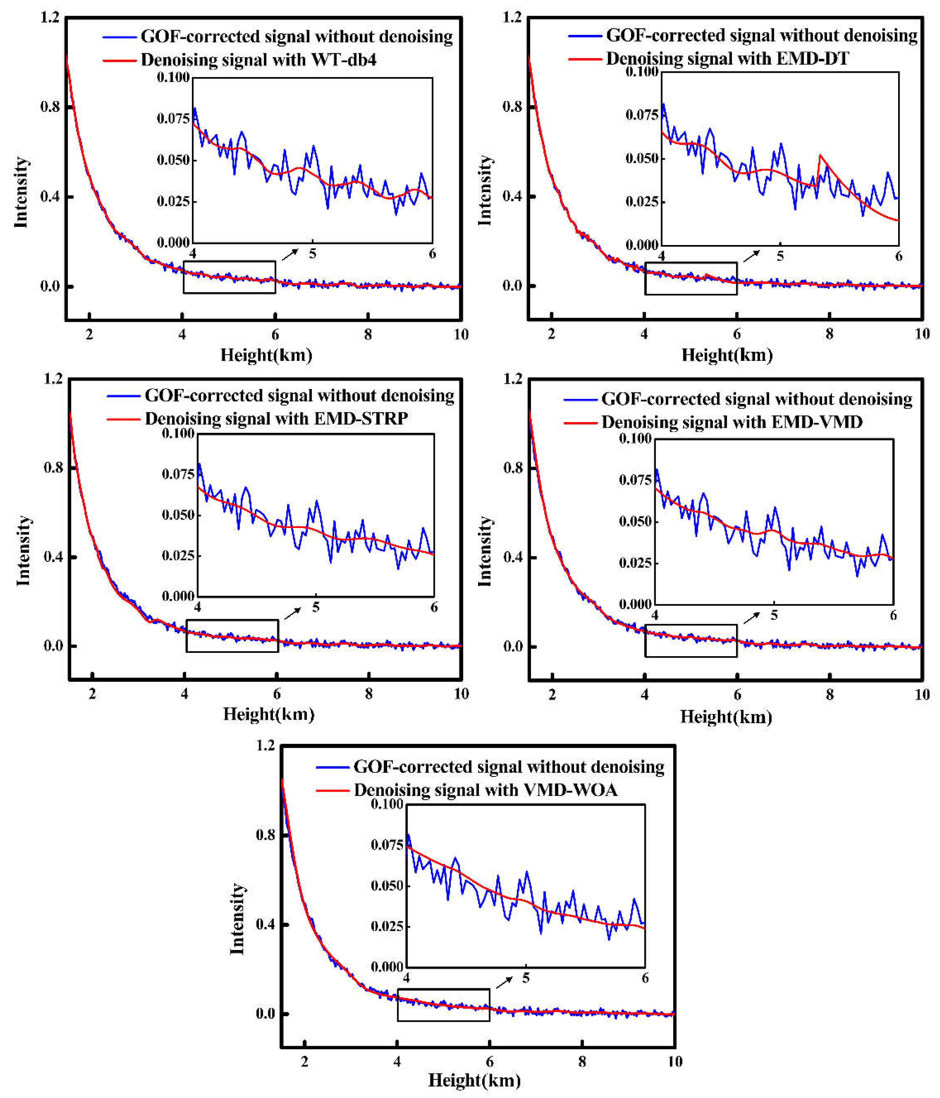
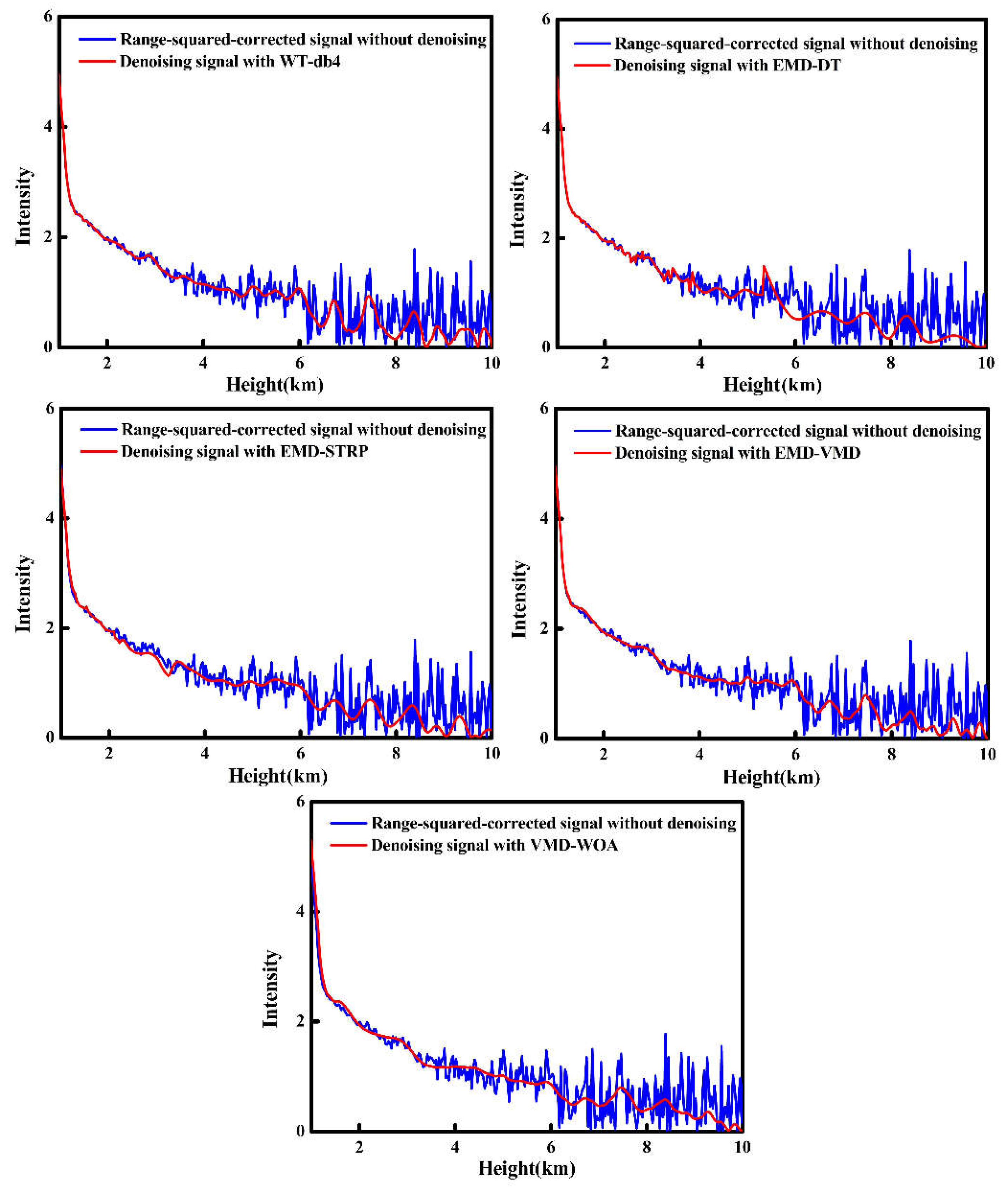
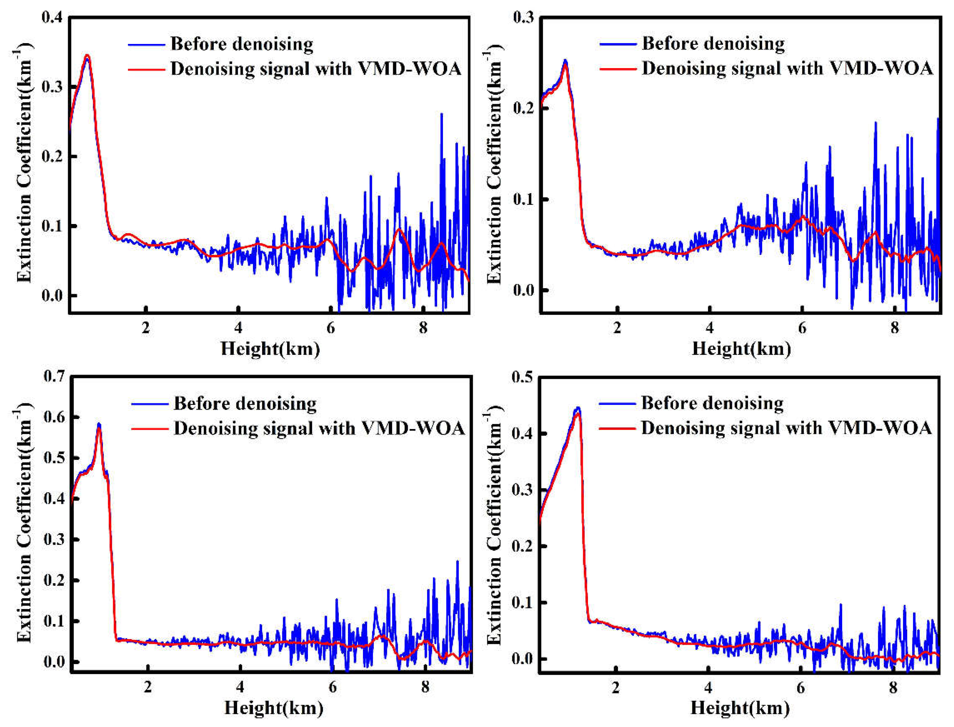
4.2. Experiments on a Lidar Echo Signal

To further verify the denoising effect of our method, we tested the proposed VMD-WOA algorithm on real cases measured by our ground-based lidar. Continuous systematic observations of the vertical distribution of aerosol extinction coefficient were conducted at the Nanjing University of Information Science (32.2 °N, 118.7 °E). The Rayleigh–Raman–Mie lidar used in the experiment was developed by the Anhui Institute of Optics and Fine Mechanics, Chinese Academy of Sciences. This lidar system contains a diode-pumped Nd:YAG laser with a pulse output wavelength of 532 nm, a repetition frequency of 20 Hz, and a pulse energy of about 200 mJ. The receiver unit is a 400 mm diameter Cassegrain telescope with a field of view of 2 mrad. The lidar echo signal is received by a photomultiplier tube and sampled at a range resolution of 30 m.

Given the different axes of the lidar transmitting and receiving system, the telescope can receive only a part of the echo at a certain distance. Thus, we corrected the geometric overlap factor (GOF) for the original lidar echo signal (measured on 24 March 2017). The waveform of the GOF-corrected signal fluctuated obviously under the influence of noise. The performance of the VMD-WOA method and the other techniques on the GOF-corrected signal is shown in Figure 8. To show the denoising results clearly, a zoomed figure of the 4–6 km signal is plotted in the figure.

Table 2. The SNRs of the geometric overlap factor (GOF)-corrected signal processed by the different denoising techniques.

	WT-db4	EMD-DT	EMD-STRP	EMD-VMD	VMD-WOA
SNR (dB)	20.67	20.36	22.25	22.61	23.92

lists the SNRs of the GOF-corrected signal processed by the five denoising techniques. As shown, the denoised results from WT-db4 and EMD-DT fluctuated considerably due to the influence of the wavelet function and direct thresholding. VMD-WOA featured the highest SNR of 23.92 dB and a smoother signal, indicating a better denoising performance than the other methods. Compared with EMD’s variation and WT, VMD could separate components of similar frequencies by searching for a number of modes and their respective center frequencies, which reproduced the input signal exactly. Moreover, by adopting Wiener filtering in the Fourier domain during the optimization process, the updated mode was less affected by noisy disturbances, which made VMD more robust against noisy data.

With increasing measurement height, the intensity of the lidar return signal decays with the square of the distance. The range-square-corrected signal is generally obtained to eliminate the influence of distance on the echo signal by multiplying the square of the distance by the received signal intensity. Figure 9 shows the range-square-corrected signal before and after denoising with different denoising techniques. As seen in the figure, each method significantly denoised the signal, but VMD-WOA featured a better denoising performance with respect to the signal smoothness and integrity. It is apparent that the VMD-WOA method filtered the noise to the greatest extent and maintained the change trend of the original signal compared with the other denoising methods. As shown, when the height was increased above 3 km, the useful far-field signal intensity decreased and was gradually overwhelmed by noise. At a height above 6 km, the signal began to weaken, with an intensity close to zero. After denoising with VMD-WOA, a useful signal above 6 km was effectively extracted, and the effective detection range of the lidar extended from 6 km to 10 km.

Then, the Fernald method was used to retrieve the profiles of the aerosol extinction coefficient, and the results are shown in Figure 10. The lidar data used for inversion were measured on 24, 25, 18, and 19 March 2017. As shown in the figure, VMD-WOA had a good noise filtering effect for the lidar echo data acquired in different time periods. This is due to the fact that VMD-WOA is an adaptive model that can select appropriate parameters according to the characteristics of the different lidar data. In fact, this method also had a good noise filtering effect for signals obtained in different locations and weather conditions, which shows that it had strong adaptability.

5. Conclusions

In this study, the noise filtering method VMD-WOA was proposed and successfully applied in the field of laser atmospheric detection. When implementing the VMD for signal processing, the decomposition mode number K and quadratic penalty α need to be selected appropriately. To solve this problem, WOA was used to search for the optimal combination of parameters (K, α). Then, the VMD-WOA method achieved denoising by reconstructing the relevant modes, which were selected using the Bhattacharyya distance. Finally, the feasibility of the proposed method was investigated theoretically and experimentally. The simulation of the filtering effects on four representative signals (Bumps, Heavy Sine, Blocks, and Doppler signals) with different SNR_in showed that the VMD-WOA method outperformed other denoising methods (WT-db4, EMD-IT, EMD-STRP, and EMD-VMD). Experimentally, the performance of VMD-WOA was compared with that of the other four methods on a lidar echo signal. The signal-to-noise ratio of the denoised signal was increased to 23.92 dB, and the detection range was extended from 6 to 10 km. Experiments on different aerosols were also carried out, and the aerosol extinction coefficient retrieved from the denoised signal showed good smoothness.

References

1. Mao, J. Noise reduction for lidar returns using local threshold wavelet analysis. Opt. Quant. Electron. 2012, 43, 59–68. [Google Scholar] [CrossRef]
2. Veerabuthiran, S.; Razdan, A.K.; Jindal, M.K.; Dubey, D.K.; Sharma, R.C. Mie lidar observations of lower tropospheric aerosols and clouds. Spectrochim. Acta A 2011, 84, 32–36. [Google Scholar] [CrossRef] [PubMed]
3. Xia, H.; Shangguan, M.; Wang, C.; Shentu, G.; Qiu, J.; Zhang, Q.; Dou, X.; Pan, J. Micro-pulse upconversion Doppler lidar for wind and visibility detection in the atmospheric boundary layer. Opt. Lett. 2016, 41, 5218. [Google Scholar] [CrossRef] [PubMed] [Green Version]
4. Zhou, Z.; Hua, D.; Wang, Y.; Yan, Q.; Li, S.; Li, Y.; Wang, H. Improvement of the signal to noise ratio of Lidar echo signal based on wavelet de-noising technique. Opt. Lasers Eng. 2013, 51, 961–966. [Google Scholar] [CrossRef]
5. Tian, P.; Cao, X.; Liang, J.; Zhang, L.; Yi, N.; Wang, L.; Cheng, X. Improved empirical mode decomposition based denoising method for lidar signals. Opt. Commun. 2014, 325, 54–59. [Google Scholar] [CrossRef]
6. Rye, B.J.; Hardesty, R.M. Nonlinear Kalman filtering techniques for incoherent backscatter lidar: Return power and log power estimation. Appl. Opt. 1989, 28, 3908–3917. [Google Scholar] [CrossRef] [PubMed]
7. Rocadenbosch, F.; Soriano, C.; Comerón, A.; Baldasano, J. Lidar inversion of atmospheric backscatter and extinction-to-backscatter ratios by use of a Kalman filter. Appl. Opt. 1999, 38, 3175–3189. [Google Scholar] [CrossRef] [PubMed]
8. Wu, S.; Liu, Z.; Liu, B. Enhancement of lidar backscatters signal-to-noise ratio using empirical mode decomposition method. Opt. Commun. 2006, 267, 137–144. [Google Scholar] [CrossRef]
9. Li, M.; Jiang, L.; Xiong, X. A novel EMD selecting thresholding method based on multiple iteration for denoising LIDAR signal. Opt. Rev. 2015, 22, 477–482. [Google Scholar] [CrossRef]
10. Tang, B.; Dong, S.; Song, T. Method for eliminating mode mixing of empirical mode decomposition based on the revised blind source separation. Signal Process. 2012, 92, 248–258. [Google Scholar] [CrossRef]
11. Dragomiretskiy, K.; Zosso, D. Variational Mode Decomposition. IEEE Trans. Signal Process. 2014, 62, 531–544. [Google Scholar] [CrossRef]
12. Wang, Y.; Markert, R.; Xiang, J.; Zheng, W. Research on variational mode decomposition and its application in detecting rub-impact fault of the rotor system. Mech. Syst. Signal Process. 2015, 60–61, 243–251. [Google Scholar] [CrossRef]
13. Wang, D.; Luo, H.; Grunder, O.; Lin, Y. Multi-step ahead wind speed forecasting using an improved wavelet neural network combining variational mode decomposition and phase space reconstruction. Renew. Energy 2017, 113, 1345–1358. [Google Scholar] [CrossRef]
14. An, X.; Yang, J. Denoising of hydropower unit vibration signal based on variational mode decomposition and approximate entropy. Trans. Inst. Meas. Control. 2015, 38, 282–292. [Google Scholar] [CrossRef]
15. Yi, C.; Lv, Y.; Dang, Z. A Fault Diagnosis Scheme for Rolling Bearing Based on Particle Swarm Optimization in Variational Mode Decomposition. Shock Vib. 2016, 2016, 1–10. [Google Scholar] [CrossRef]
16. Li, Z.; Chen, J.; Zi, Y.; Pan, J. Independence-oriented VMD to identify fault feature for wheel set bearing fault diagnosis of high speed locomotive. Mech. Syst. Signal Process. 2017, 85, 512–529. [Google Scholar] [CrossRef]
17. Shi, P.; Yang, W. Precise feature extraction from wind turbine condition monitoring signals by using optimised variational mode decomposition. IET Renew. Power Gen. 2017, 11, 245–252. [Google Scholar] [CrossRef]
18. Li, Y.; Li, Y.; Chen, X.; Yu, J. Research on Ship-Radiated Noise Denoising Using Secondary Variational Mode Decomposition and Correlation Coefficient. Sensors 2018, 18, 48. [Google Scholar]
19. Li, Y.; Li, Y.; Chen, X.; Yu, J. Denoising and Feature Extraction Algorithms Using NPE Combined with VMD and Their Applications in Ship-Radiated Noise. Symmetry 2017, 9, 256. [Google Scholar] [CrossRef]
20. Ma, W.; Yin, S.; Jiang, C.; Zhang, Y. Variational mode decomposition denoising combined with the Hausdorff distance. Rev. Sci. Instrum. 2017, 88, 35109. [Google Scholar] [CrossRef]
21. Chang, J.; Zhu, L.; Li, H.; Xu, F.; Liu, B.; Yang, Z. Noise reduction in Lidar signal using correlation-based EMD combined with soft thresholding and roughness penalty. Opt. Commun. 2018, 407, 290–295. [Google Scholar] [CrossRef]
22. Liu, Y.; Yang, G.; Li, M.; Yin, H. Variational mode decomposition denoising combined the detrended fluctuation analysis. Signal Process. 2016, 125, 349–364. [Google Scholar] [CrossRef]
23. Mirjalili, S.; Lewis, A. The Whale Optimization Algorithm. Adv. Eng. Softw. 2016, 95, 51–67. [Google Scholar] [CrossRef]
24. Hasanien, H.M. Performance improvement of photovoltaic power systems using an optimal control strategy based on whale optimization algorithm. Electr. Power Syst. Res. 2018, 157, 168–176. [Google Scholar] [CrossRef]
25. Huang, J.; Hu, X.; Geng, X. An intelligent fault diagnosis method of high voltage circuit breaker based on improved EMD energy entropy and multi-class support vector machine. Electr. Power Syst. Res. 2011, 81, 400–407. [Google Scholar] [CrossRef]
26. Li, K.; Su, L.; Wu, J.; Wang, H.; Chen, P. A Rolling Bearing Fault Diagnosis Method Based on Variational Mode Decomposition and an Improved Kernel Extreme Learning Machine. Appl. Sci. 2017, 7, 1004. [Google Scholar] [CrossRef]
27. Komaty, A.; Boudraa, A.; Augier, B.; Dare-Emzivat, D. EMD-Based Filtering Using Similarity Measure Between Probability Density Functions of IMFs. IEEE Trans. Instrum. Meas. 2014, 63, 27–34. [Google Scholar] [CrossRef] [Green Version]
Figure 1. Flowchart of the proposed variational mode decomposition (VMD)-whale optimization algorithm (WOA). PDF is probability density function.
Remotesensing 11 00126 g001
Figure 2. The four types of synthetic signal with SNRin = 5 dB.
Remotesensing 11 00126 g002
Figure 3. WOA convergence curve for VMD parameter optimization.
Remotesensing 11 00126 g003
Figure 4. Decomposition result of the noisy Bumps signal.
Remotesensing 11 00126 g004
Figure 5. Bhattacharyya distance between modes and the Bumps signal. BLIMF is band-limited intrinsic mode function.
Remotesensing 11 00126 g005
Figure 6. Comparisons of different denoising techniques for the noisy Bumps signal. WT is wavelet transform, EMD is empirical mode decomposition, EMD-DT is EMD-direct thresholding, EMD-STRP is EMD combined with soft thresholding and a roughness penalty, EMD-VMD is the VMD method based on the decomposition level of EMD, and VMD-WOA is the VMD method combined with the whale optimization algorithm (WOA).
Remotesensing 11 00126 g006
Figure 7. Denoising performance with different SNRin on the noisy Bumps signal.
Remotesensing 11 00126 g007
Figure 8. Comparison of denoising results from the proposed VMD-WOA and the other methods. GOF is geometric overlap factor.
Remotesensing 11 00126 g008
Figure 9. Comparison of the VMD-WOA and the other methods for the range-squared-corrected signal.
Remotesensing 11 00126 g009
Figure 10. Comparison of aerosol extinction coefficient profiles from different observation times.
Remotesensing 11 00126 g010