Hyperspectral Feature Extraction Using Sparse and Smooth Low-Rank Analysis

Abstract

In this paper, we develop a hyperspectral feature extraction method called sparse and smooth low-rank analysis (SSLRA). First, we propose a new low-rank model for hyperspectral images (HSIs) where we decompose the HSI into smooth and sparse components. Then, these components are simultaneously estimated using a nonconvex constrained penalized cost function (CPCF). The proposed CPCF exploits total variation penalty, ${\ell }_1$ penalty, and an orthogonality constraint. The total variation penalty is used to promote piecewise smoothness, and, therefore, it extracts spatial (local neighborhood) information. The ${\ell }_1$ penalty encourages sparse and spatial structures. Additionally, we show that this new type of decomposition improves the classification of the HSIs. In the experiments, SSLRA was applied on the Houston (urban) and the Trento (rural) datasets. The extracted features were used as an input into a classifier (either support vector machines (SVM) or random forest (RF)) to produce the final classification map. The results confirm improvement in classification accuracy compared to the state-of-the-art feature extraction approaches.

1. Introduction

Hyperspectral cameras can acquire remotely sensed images for a large number of contiguous spectral bands. Thus, a hyperspectral image (HSI) contains detailed spectral information of a scene. Since many kinds of materials have unique spectral signatures, this type of image is useful for recognizing the types of materials in a captured scene [1]. On the other hand, due to the Hughes effect [2], which is also known as the curse of dimensionality, the high spectral dimensionality makes the analysis of HSIs a challenging task from both computational and statistical perspective. The limited availability of training samples is a common issue in this kind of analysis since their collection can be both time demanding and expensive [3]. An increase in the number of spectral features, after a certain point, usually causes a decrease in classification accuracy when the number of training samples is limited. As a result, reducing the spectral dimensionality (or feature reduction) is of great interest in HSI analysis [4]. In general, dimensionality reduction (DR) techniques can be divided into feature selection (FS) and feature extraction (FE). In this paper, we focus on FE.

FE is the process of finding a set of vectors that represent an observation while reducing the dimensionality. For data classification, it is desirable to extract informative features that are useful for differentiating between classes of interest. Although DR is important for HSI analysis, the error due to the reduction in dimension has to occur without sacrificing the discriminative power of the classifier [5].

FE techniques can be broadly divided, based on the availability of training data, into two main groups: supervised FE (SFE) and unsupervised FE (USFE). The SFE methods require training samples while the USFE techniques are used to extract distinctive features in the absence of labeled training data.

SFE has been widely studied in the hyperspectral community [1]. Discriminant analysis feature extraction (DAFE) [6] is a classical SFE approach. It is a parametric method that extracts features that maximize the proportion of the between-class variance to within-class variance. The main shortcoming of DAFE is that this approach is not full rank and its rank at maximum is equal to the number of classes minus one. In addition, the class mean values can highly affect the performance of DAFE. Therefore, decision boundary feature extraction (DBFE) [7] and nonparametric weighted feature extraction (NWFE) [8] are suggested for HSI classification. In DBFE, the decision boundary is defined by applying the Bayes decision rules on the training samples and from that a decision boundary matrix transformation is calculated to extract the feature vectors. Hence, DBFE could fail in the case of having too few training samples since it directly works with the training samples to determine the location of the effective decision boundaries. NWFE is designed to improve the limitations of parametric feature extraction by putting different weights on samples to compute the local means and define a new nonparametric between-class and within-class scatter matrices to produce more features than DAFE. In addition, discriminant analysis based techniques such as the linear constraint distance-based discriminant analysis (LCDA) [9], the modified Fisher’s linear discriminant analysis (MFLDA) [10], and a tensor representation-based discriminant analysis [11] were all proposed to improve the performance of the DAFE.

Recent SFE approaches take the advantage of the local neighborhood properties (spatial information) of data. Li et al. [12] considered local Fisher’s discriminant analysis [13] to perform DR while preserving the corresponding multi-modal structure. In [14], local neighborhood information is taken into account in both spectral and spatial domains to obtain a discriminative projection for dimensionality reduction of hyperspectral data. Xue et al. [15] introduced a nonlinear FE approach based on spatial and spectral regularized local discriminant embedding to address spatial variability and spectral multi-modality.

USFE techniques are usually based on optimizing an objective function to project the original features into a lower dimensional feature space. Principal component analysis (PCA) searches for a projection to maximize the signal variance [16]. Maximum noise fraction (MNF) [17] and noise adjusted principal components (NAPC) [18] seek a projection that maximizes the signal-to-noise ratio (SNR). Such FE approaches are mostly used for data representation, usually as a preprocessing step, and address the large size of hyperspectral datasets. Independent component analysis (ICA) [19,20], non-negative matrix factorization (NMF) [21,22], and hyperspectral unmixing [23,24] are other examples of USFE techniques.

Some FE techniques are proposed based on preserving local (spatial) information [25,26]. Neighborhood preserving embedding (NPE) [27], locality preserving projection (LPP) [28] and linear local tangent space alignment (LLTSA) [29] are proposed for hyperspectral FE [30,31]. The work in [32] develops a tensor version of the LPP algorithm for hyperspectral DR and classification. The work in [33] proposes a common minimization framework called graph-embedding (GE), which is based on estimating an undirected weighted graph to describe the desired intrinsic (statistical or geometrical) properties of the data. The method uses either scale normalization or penalty graph constraints that describe undesirable properties. In [34], a sparse graph-based discriminant analysis (SGDA) technique that induces sparsity on the graph construction is proposed for hyperspectral DR and classification. SGDA may not obtain acceptable results when the input data have a nonlinear and complex nature. To address this issue, a kernel extension of SGDA is proposed in [35]. Image fusion and recursive filtering [36] are designed in [37], which incorporate spatial information to extract informative features. In [38], a DR approach is developed to estimate a sparse and low-rank projection matrix by fulfilling the restricted isometric property condition on all secants of hyperspectral data to preserve the nearest neighbor points of all pixels to improve the subsequent classification step further. Total variation (TV) regularization is suggested in [39] for HSI feature extraction. Wavelet-based sparse reduced-rank regression [40] and sparse and low-rank modeling [41] are suggested for hyperspectral feature extraction. Recently, in [42], orthogonal total variation component analysis (OTVCA) is proposed, where a non-convex cost function is optimized to find the best representation for HSI in a low dimensional feature space while controlling the spatial smoothness of the features by using a TV regularization. The TV penalty promotes piecewise smoothness (homogeneous spatial regions) on the extracted features, and thus substantially helps to extract spatial (local neighborhood) information that is very useful for classification.

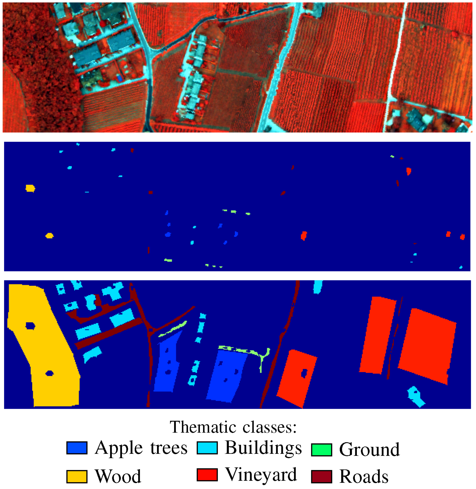
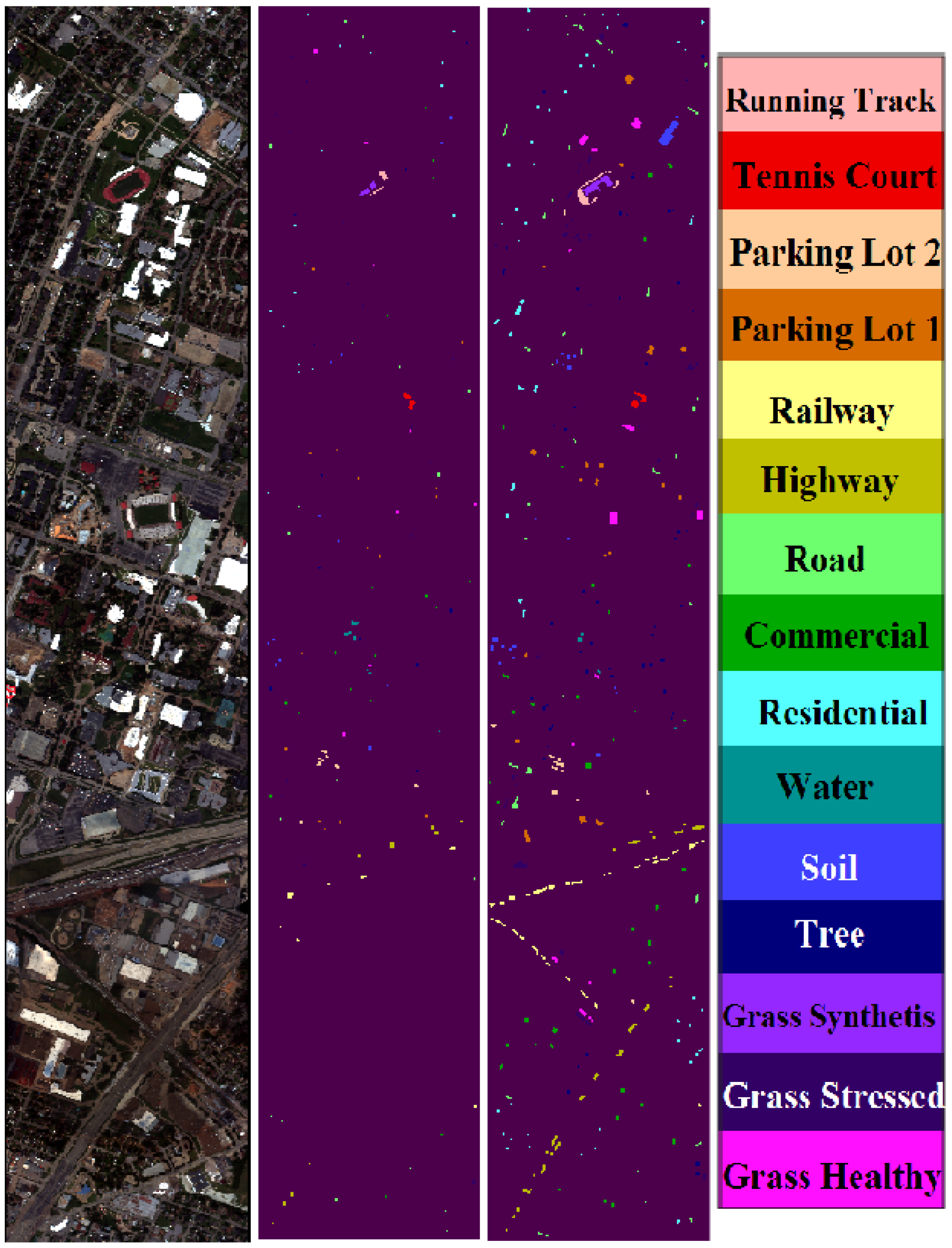
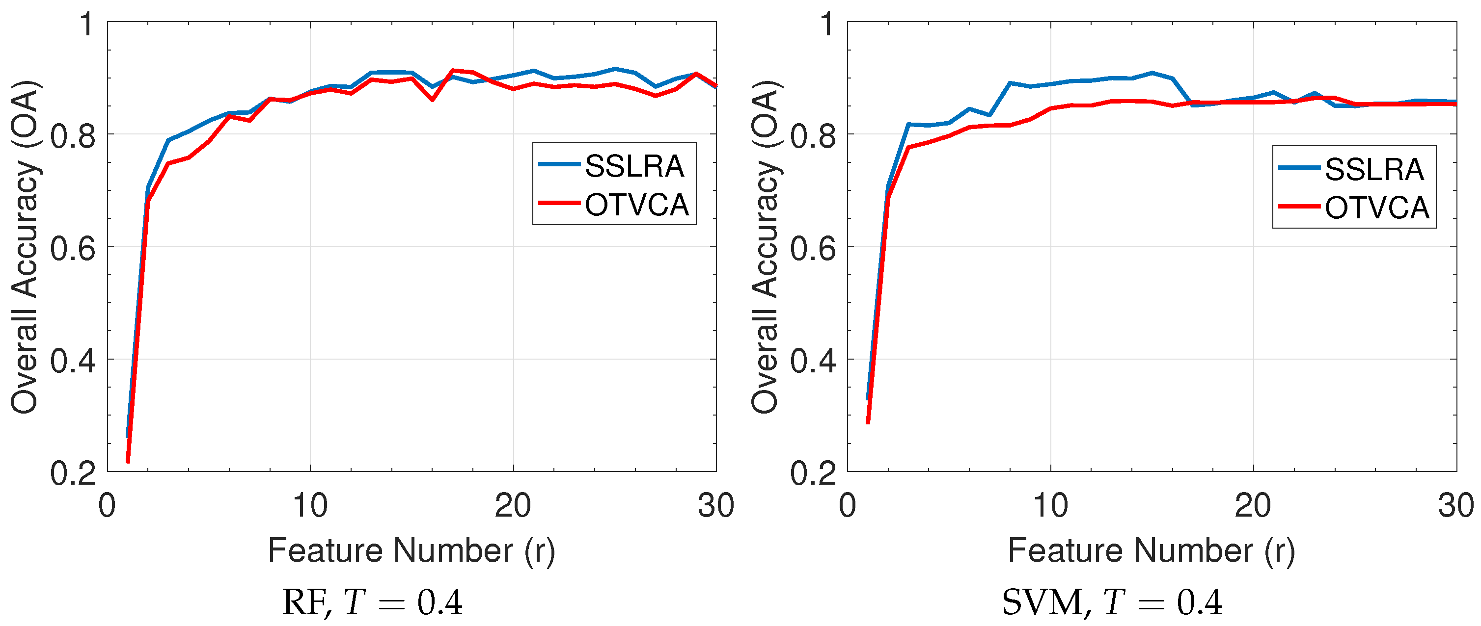
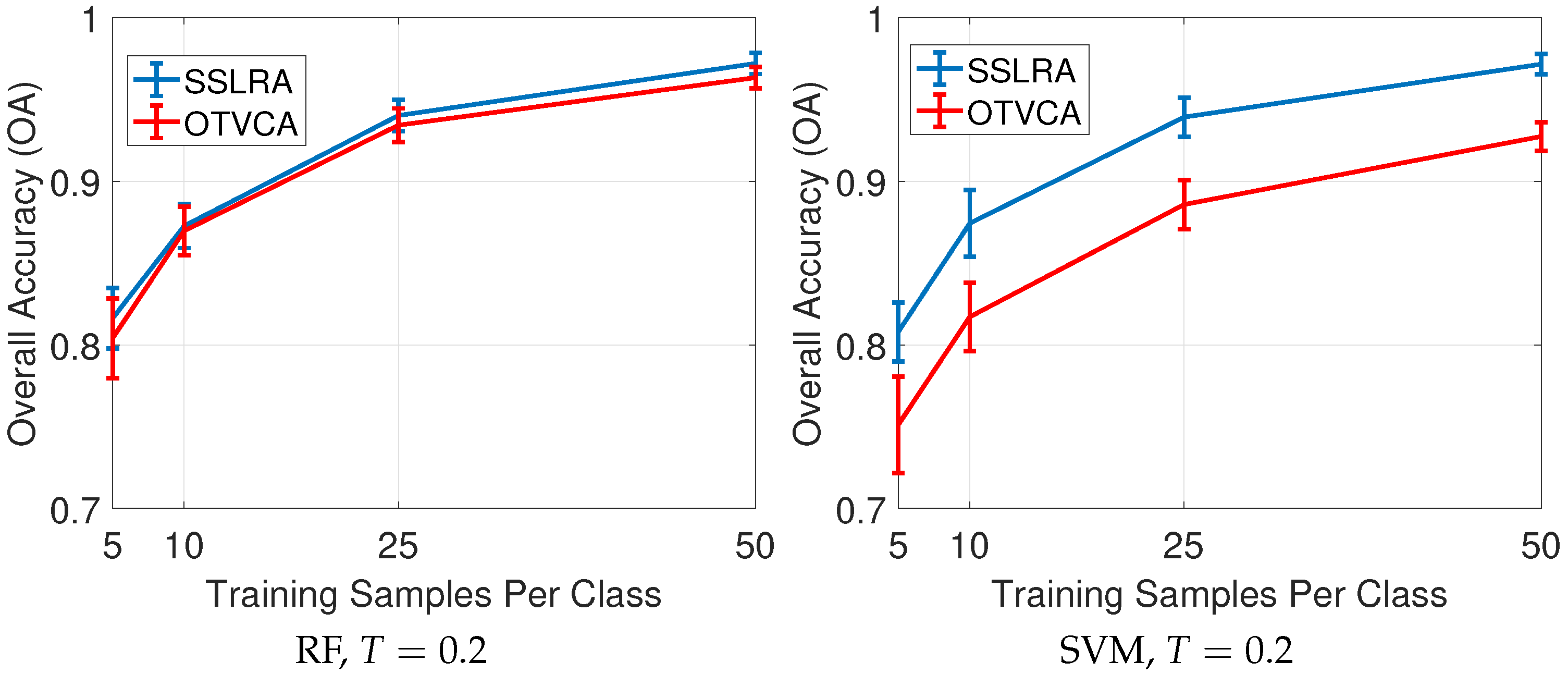
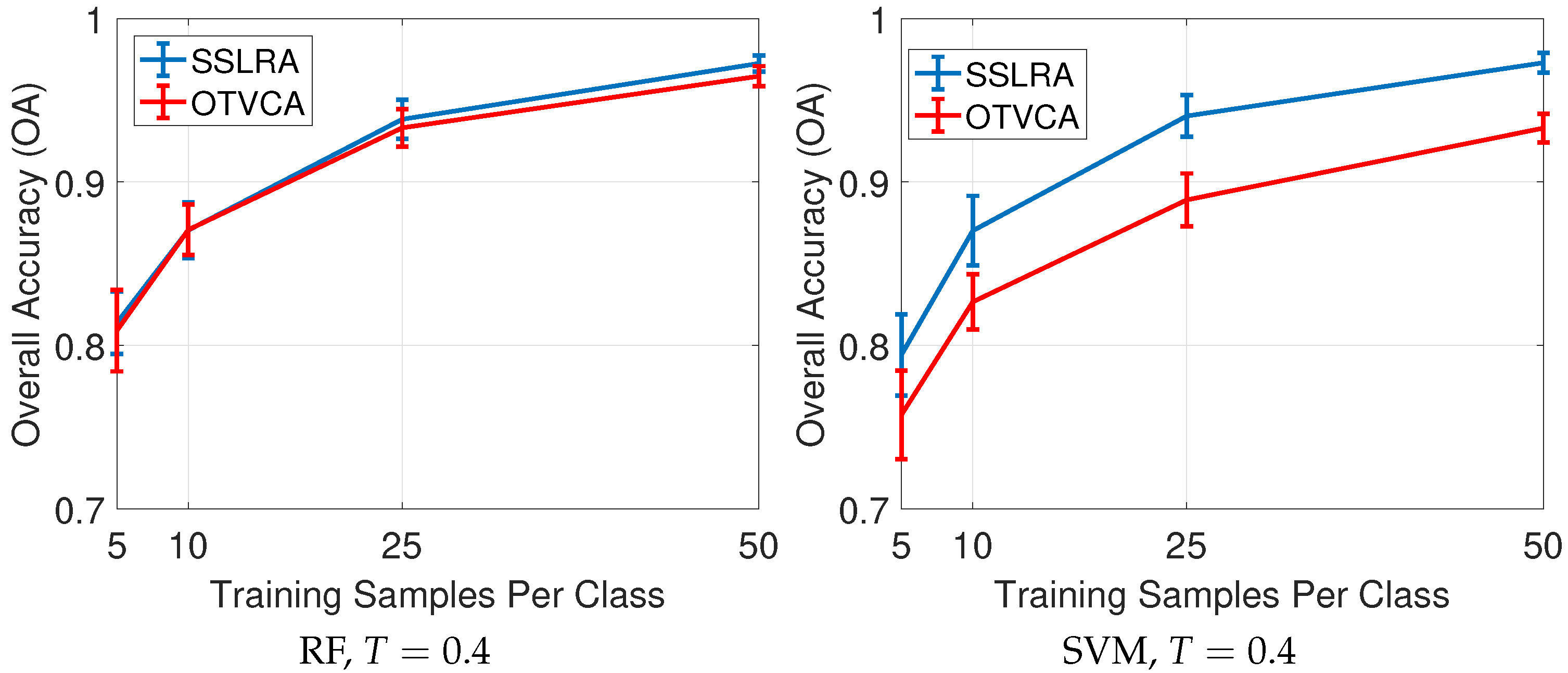
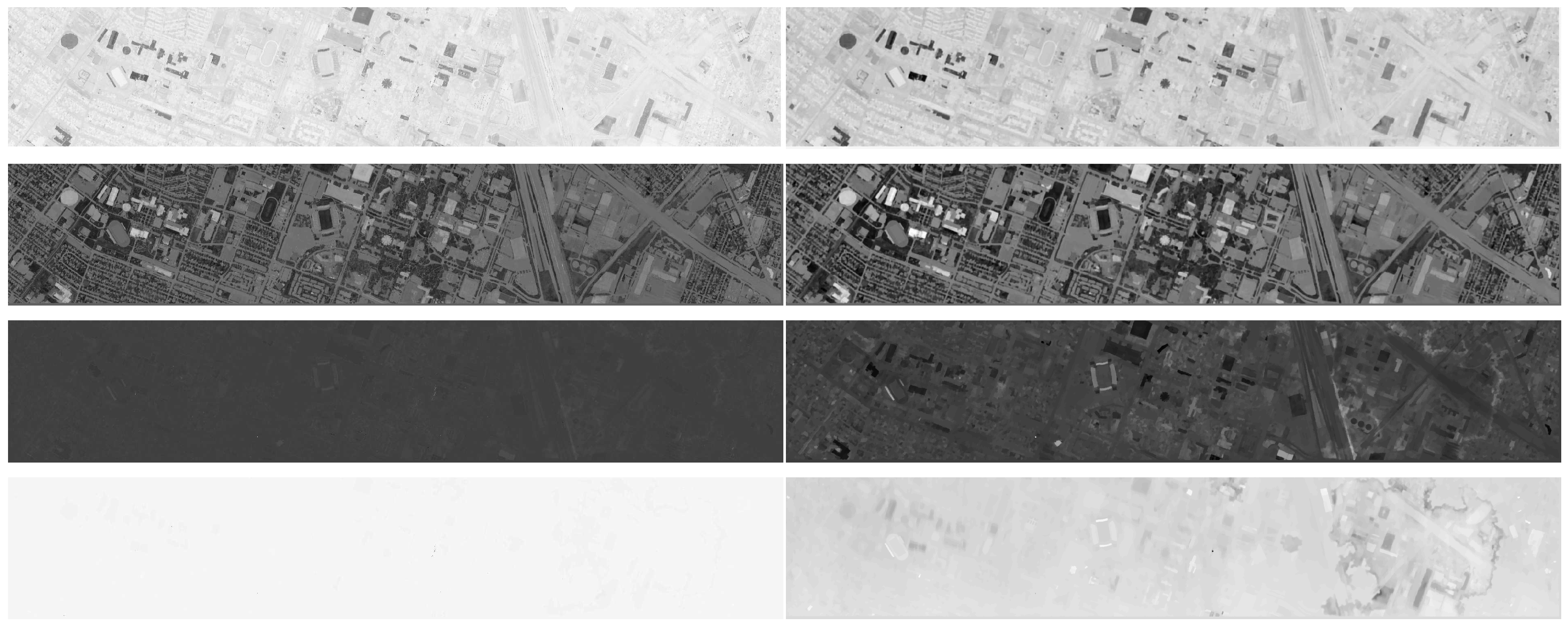
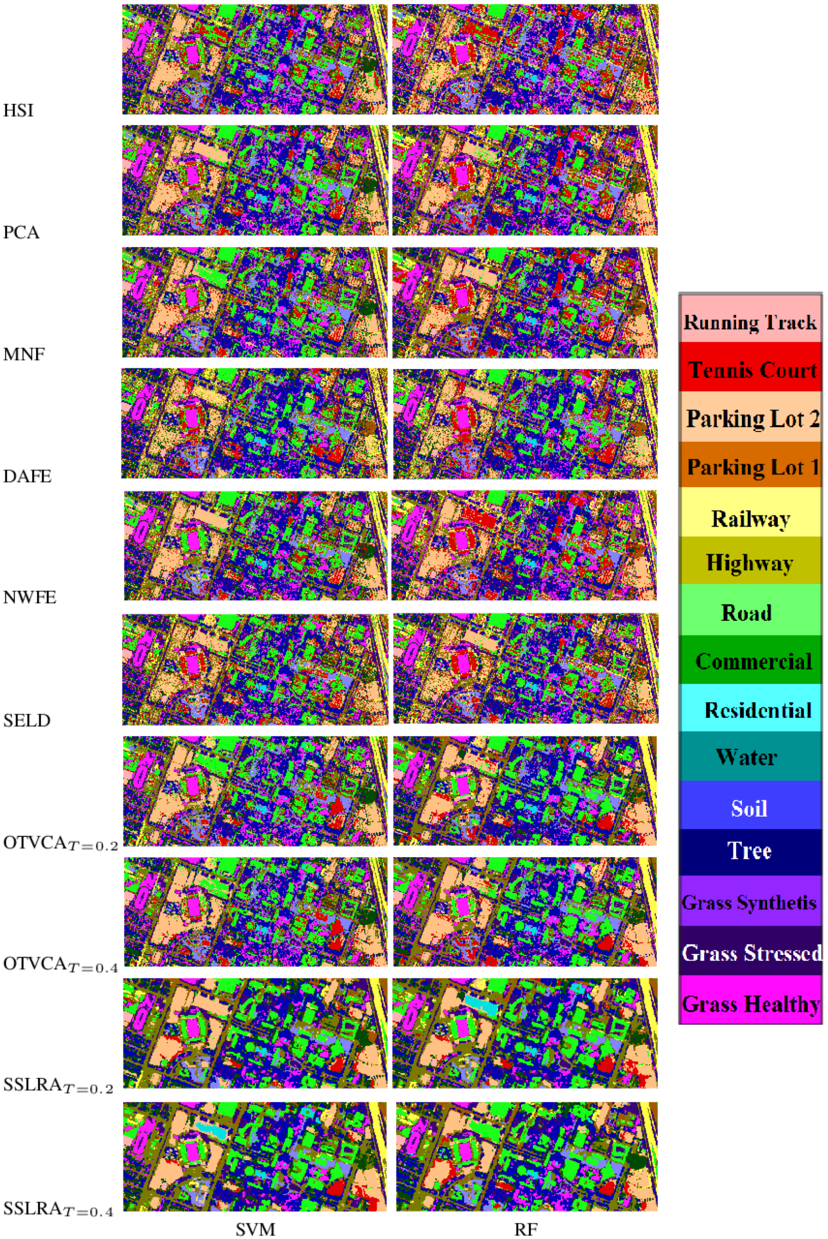
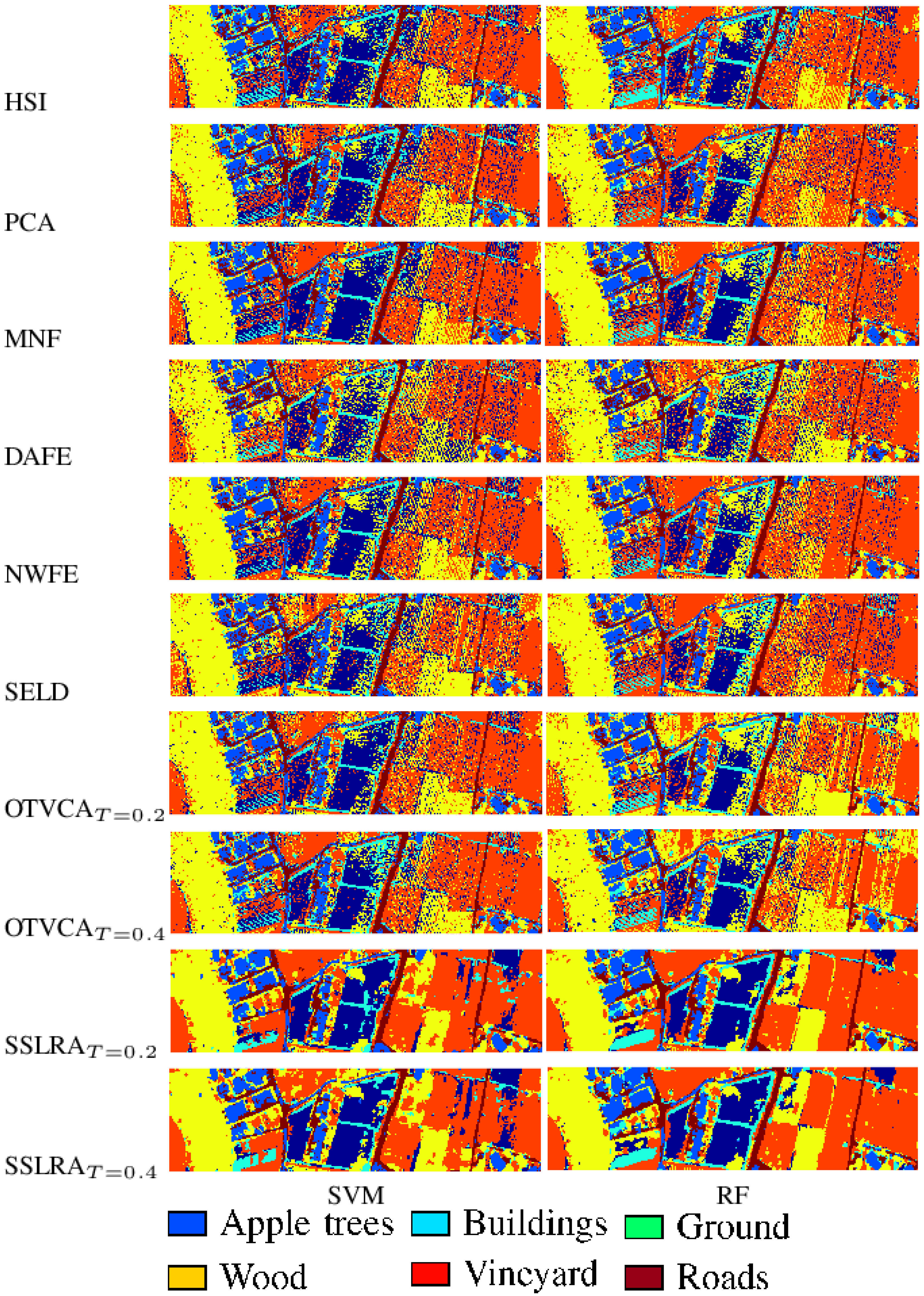
In this paper, we propose a USFE for the classification of HSI called sparse and smooth low-rank analysis (SSLRA). SSLRA decomposes the HSI into sparse and piecewise smooth components. To capture the spectral redundancy of HSI and perform DR, we assume that these components can be represented in a lower dimensional space. Therefore, we propose a low-rank model for HSI in which the HSI is modeled based on a combination of sparse and smooth components. The components are estimated simultaneously by optimizing a constrained penalized cost function (CPCF). The TV and ${\ell }_1$ penalties are exploited by the CPCF to promote the smoothness and the sparsity of the corresponding components, respectively. We assume that the unknown bases are orthogonal, and therefore we solve the CPCF by enforcing an orthogonality constraint. In the experiments, we used two HSIs: (1) an urban HSI of the University of the Houston campus; and (2) a rural HSI of the Italian city of Trento. The experiments confirmed that SSLRA outperforms both OTVCA and state-of-the-art FE techniques concerning classification accuracy.

The organization of the paper is as follows. The proposed hyperspectral feature extraction technique (SSLRA) and the corresponding algorithm are derived and explained in Section 2. Section 3 is devoted to the experimental results. Finally, Section 4 concludes the paper.

Notation

The notations used in this paper are as follows. The number of spectral bands and pixels in each band are denoted by p and n, respectively. r indicates the rank of the HSI. Matrices are represented by bold and capital letters, vectors by bold letters, the $(i,j)$th element of $\mathbf{X}$ by $x_{ij}$, and the ith column by ${\mathbf{x}}_{\left(i\right)}$. ${\mathbf{I}}_p$ denotes identity matrix of size $p\times p$. $\hat{\mathbf{X}}$ stands for the estimate of $\mathbf{X}$. The Frobenius norm and TV-normare denoted by ${∥.∥}_F$ and ${∥.∥}_{T\mathrm{TV}}$, respectively. The definitions of the symbols used in the paper are given in

Table 1. The definitions of the symbols used in this paper.

Sym.	Definition
$x_i$	the ith entry of the vector $\mathbf{x}$
$x_{ij}$	the $(i,j)$th entry of the matrix $\mathbf{X}$
${\mathbf{x}}_{\left(i\right)}$	the ith column of the matrix $\mathbf{X}$
${\mathbf{x}}_j^T$	the jth row of the matrix $\mathbf{X}$
${∥\mathbf{x}∥}_1$	$l_1$-norm of the vector $\mathbf{x}$, obtained by ${\sum }_i\left|x_i\right|$
${∥\mathbf{x}∥}_2$	$l_2$-norm of the vector $\mathbf{x}$, obtained by $\sqrt{{\sum }_i{x}_i^2}$
${∥\mathbf{X}∥}_1$	$l_1$-norm of the matrix $\mathbf{X}$, obtained by ${\sum }_{i,j}\left|{\mathbf{x}}_{ij}\right|$
${∥\mathbf{X}∥}_F$	Frobenius-norm of the matrix $\mathbf{X}$, obtained by $\sqrt{{\sum }_{i,j}{x}_{ij}^2}$
$\hat{\mathbf{X}}$	the estimate of the variable $\mathbf{X}$
${∥\mathbf{x}∥}_{TV}$	Total variation norm (explained in Appendix A)

.

2. Hyperspectral Modeling and Sparse and Smooth Low-Rank Analysis

HSIs are often represented by using low-rank models. Such models have, for example, been shown to be more appropriate for HSI in terms of mean squared error than full-rank models [41]. However, the rank is unknown and has to be estimated [43,44]. We model the observed HSI as

$$\mathbf{Y}=\mathbf{X}+\mathbf{N},$$

(1)

where $\mathbf{Y}=\left[{\mathbf{y}}_{\left(i\right)}\right]$ is an $n\times p$ matrix containing the vectorized observed image at band i in its ith column, $\mathbf{X}=\left[{\mathbf{x}}_{\left(i\right)}\right]$ is an $n\times p$ matrix representing the HSI, and $\mathbf{N}=\left[{\mathbf{n}}_{\left(i\right)}\right]$ is an $n\times p$ matrix that represents the noise and model error. Here, we assume that $\mathbf{X}$ is a low-rank matrix, i.e., it has rank $r<<\min (n,p)$. The low-rank property can be enforced by representing $\mathbf{X}$ as a product of two rank r matrices $(\mathbf{F}+\mathbf{S})$ and ${\mathbf{V}}^T$, which leads to the following low-rank model:

$$\mathbf{Y}=(\mathbf{F}+\mathbf{S}){\mathbf{V}}^T+\mathbf{N},$$

(2)

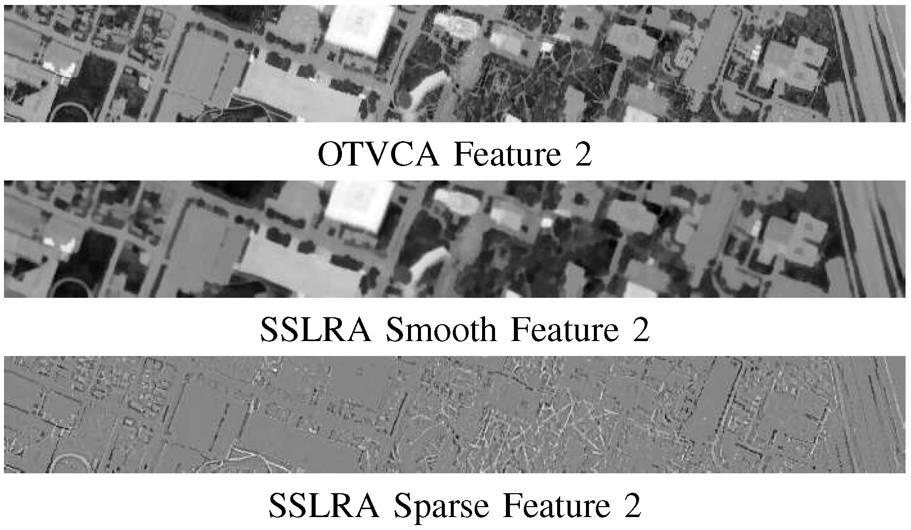
where $\mathbf{F}=\left[{\mathbf{f}}_{\left(i\right)}\right]$ and $\mathbf{S}=\left[{\mathbf{s}}_{\left(i\right)}\right]$ are matrices of size $n\times r$ containing the unknown smooth and sparse components, respectively, and $\mathbf{V}$ is an unknown $p\times r$ subspace matrix. The model in Equation (2) separates the sparse features from the smooth features. The smooth features can be used to promote smooth regions of interests in the classification maps.

Assuming the model in Equation (2), we propose a CPCF to simultaneously estimate $\mathbf{F}$, $\mathbf{S}$, and $\mathbf{V}$ by solving

$$\underset{\mathbf{F},\mathbf{S},\mathbf{V}}{min}J\left(\mathbf{F},\mathbf{S},\mathbf{V}\right)\mathrm{s.t.}{\mathbf{V}}^T\mathbf{V}={\mathbf{I}}_r,$$

(3)

where

$$J\left(\mathbf{F},\mathbf{S},\mathbf{V}\right)=\frac{1}{2}{∥\mathbf{Y}-(\mathbf{F}+\mathbf{S}){\mathbf{V}}^T∥}_F^2+{\lambda }_1\sum _{i=1}^r{∥{\mathbf{f}}_{\left(i\right)}∥}_{\mathrm{TV}}+{\lambda }_2{∥\mathbf{S}∥}_1.$$

In Equation (4), the TV-norm (see Appendix A) promotes piecewise smoothness on $\mathbf{F}$, the ${\ell }_1$ norm promotes sparsity on $\mathbf{S}$, and the constraint ${\mathbf{V}}^T\mathbf{V}={\mathbf{I}}_r$ enforces the orthogonality condition on the subspace. Note that minimization of Equation (3) is non-convex and therefore the solution might lead to a local minima.

To solve Equation (3), we use a cyclic descent (CD) algorithm [45,46,47] where the problem is solved with respect to one matrix at a time while the others are assumed to be fixed. As a result, the proposed CD approach consists of the four steps discussed below: initialization, the $\mathbf{F}$ step, the $\mathbf{S}$ step, and the $\mathbf{V}$ step.

2.1. Initialization

Decompose $\mathbf{Y}$ by using truncated (rank-r) singular value decomposition (SVD), i.e., $\mathrm{SVD}\left(\mathbf{Y}\right)=\mathbf{U}\mathbf{K}{\mathbf{W}}^T$. Then, initialize ${\mathbf{V}}^0=\mathbf{W}$ and $\mathbf{S}=\mathbf{0}$.

2.2. F-Step

Given fixed ${\mathbf{V}}^m$ and ${\mathbf{S}}^m$, get ${\mathbf{F}}^{m+1}$ by solving Equation (3) which can be reduced to

$$\begin{array}{c}\hfill \underset{\mathbf{F}}{min}\sum _{i=1}^r\frac{1}{2}{∥{\mathbf{g}}_{\left(i\right)}-{\mathbf{f}}_{\left(i\right)}-{\mathbf{s}}_{\left(i\right)}∥}_2^2+{\lambda }_1\sum _{i=1}^r{∥{\mathbf{f}}_{\left(i\right)}∥}_{\mathrm{TV}},\end{array}$$

(4)

where $\mathbf{G}=\left[{\mathbf{g}}_{\left(i\right)}\right]=\mathbf{Y}{\mathbf{V}}^m$. The problem in Equation (4) can be thought of as r-separable TV regularization problems [48] that can be solved using the split Bregman iterations method given in [49] (also known as the alternative direction method of multipliers (ADMM) [50]) denoted by

$${\mathbf{F}}^{m+1}=\mathrm{SplitBregman}(\mathbf{G}-{\mathbf{S}}^m,{\lambda }_1).$$

2.3. S-Step

Given fixed ${\mathbf{V}}^m$ and ${\mathbf{F}}^{m+1}$, get ${\mathbf{S}}^{m+1}$ by solving Equation (3), i.e.,

$${\mathbf{S}}^{m+1}=arg\underset{\mathbf{S}}{min}\frac{1}{2}{∥\mathbf{G}-\mathbf{F}-\mathbf{S}∥}_F^2+{\lambda }_2{∥\mathbf{S}∥}_1.$$

(5)

It can be shown that Equation (5) is separable and the solution is given by

$${\widehat{s}}_{ji}=max\left(0,\left|g_{ji}-f_{ji}\right|-{\lambda }_2\right)\frac{g_{ji}-f_{ji}}{\left|g_{ji}-f_{ji}\right|},$$

(6)

which is called soft-thresholding and often is written as

$${\hat{\mathbf{S}}}^{m+1}=\mathrm{soft}\left(\mathbf{G}-{\mathbf{F}}^{m+1},{\lambda }_2\right).$$

(7)

Note that soft function in Equation (7) is applied element-wise on matrix $\mathbf{G}-{\mathbf{F}}^{m+1}$.

2.4. V-Step

Given fixed ${\mathbf{F}}^{m+1}$ and ${\mathbf{S}}^{m+1}$, get ${\mathbf{V}}^{m+1}$ by solving Equation (3), which can be rewritten as

$$\underset{\mathbf{V}}{min}{∥\mathbf{Y}-({\mathbf{F}}^{m+1}+{\mathbf{S}}^{m+1}){\mathbf{V}}^T∥}_F^2\mathrm{s.t.}{\mathbf{V}}^T\mathbf{V}={\mathbf{I}}_r.$$

(8)

The solution is given by a low-rank Procrustes rotation [51]

$${\mathbf{V}}^{m+1}={\mathbf{PQ}}^T,$$

where the matrices $\mathbf{P}$ and $\mathbf{Q}$ are given by the following truncated SVD of rank r

$$\mathbf{P}{\mathbf{\Sigma }\mathbf{Q}}^T=\mathrm{SVD}\left({\mathbf{Y}}^T({\mathbf{F}}^{m+1}+{\mathbf{S}}^{m+1})\right),$$

where $\mathbf{\Sigma }$ is a diagonal matrix which contains the first r singular values of ${\mathbf{Y}}^T({\mathbf{F}}^{m+1}+{\mathbf{S}}^{m+1})$. The resulting algorithm is summarized in Algorithm 1.

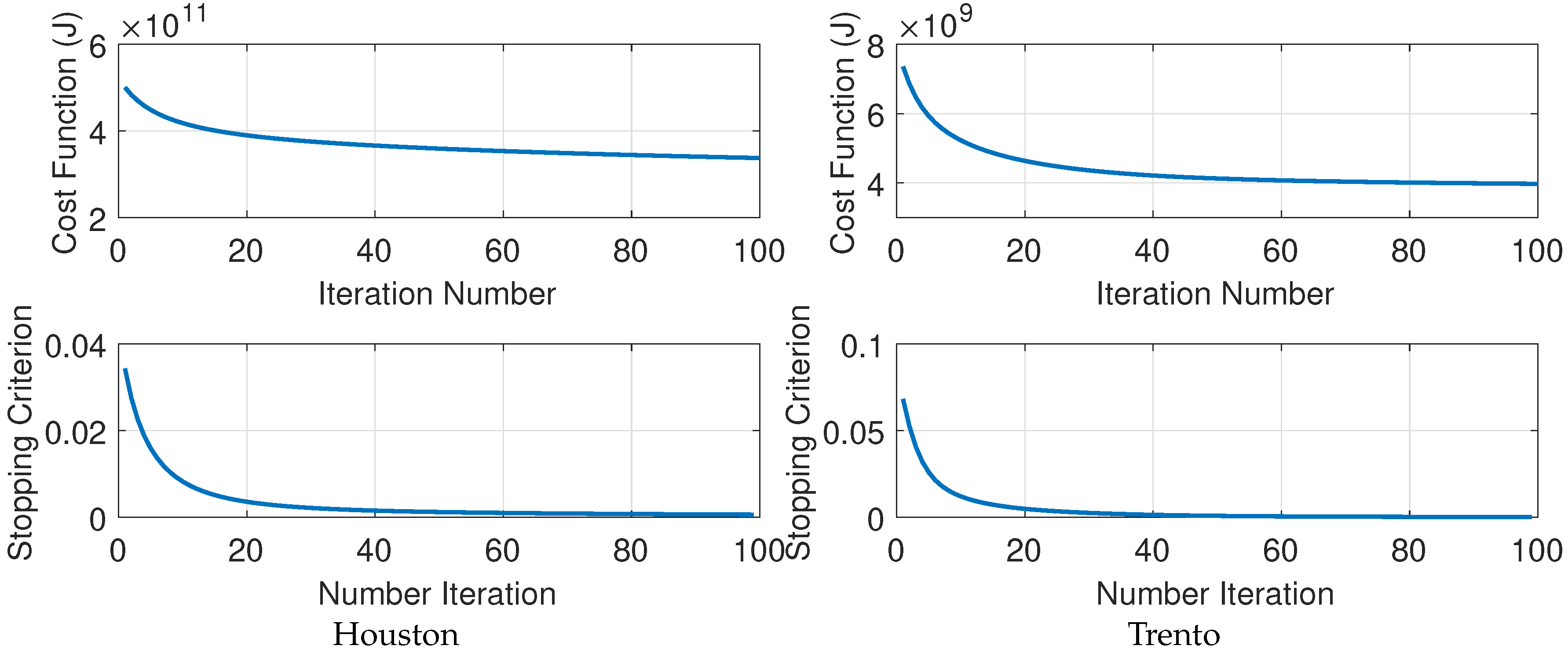
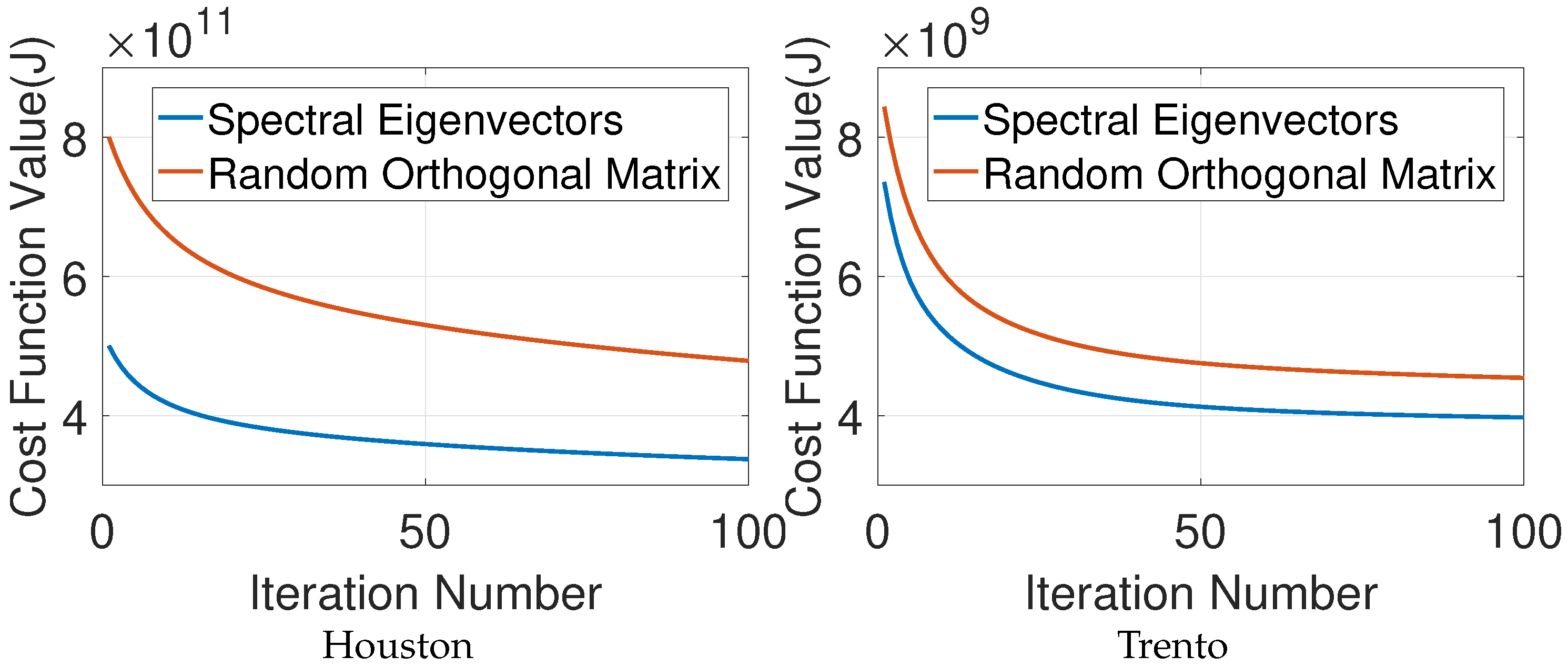
The monotonicity property of SSLRA can be observed easily since by construction the algorithm guarantees that the cost function is non-increasing with respect to the iteration index, i.e., $J\left({\mathbf{F}}^0,{\mathbf{S}}^0,{\mathbf{V}}^0\right)\ge J\left({\mathbf{F}}^1,{\mathbf{S}}^0,{\mathbf{V}}^0\right)\ge J\left({\mathbf{F}}^1,{\mathbf{S}}^1,{\mathbf{V}}^0\right)\ge J\left({\mathbf{F}}^1,{\mathbf{S}}^1,{\mathbf{V}}^1\right)\ge \dots \ge J\left({\mathbf{F}}^m,{\mathbf{S}}^m,{\mathbf{V}}^m\right)\ge J\left({\mathbf{F}}^{m+1},{\mathbf{S}}^m,{\mathbf{V}}^m\right)\ge J\left({\mathbf{F}}^{m+1},{\mathbf{S}}^{m+1},{\mathbf{V}}^m\right)\ge J\left({\mathbf{F}}^{m+1},{\mathbf{S}}^{m+1},{\mathbf{V}}^{m+1}\right)\ge 0$. Therefore, the cost function is guaranteed to decrease or stay the same at each iteration of the algorithm. Since the cost function is both upper bounded (by the initial value) and lower bounded (since it is greater than or equal zero), the cost function iterations will converge to a finite value.

Note that the smooth features ($\mathbf{F}$) extracted using SSLRA are used for classification purposes in this paper. This is discussed further in Section 3.

Algorithm 1: SSLRA.

3. Experimental Results

Two HSIs, the Houston and Trento datasets, described below, were used in the experiments. The Houston dataset investigation is presented in Section 3.2, Section 3.3 and Section 3.4. The Trento dataset experiment is presented in Section 3.4. Two classifiers were used in the experiments: Random Forest (RF) and Support Vector Machine (SVM). For the RF, we set the number of trees to 200. For the SVM, a radial basis function (RBF) kernel was used. The penalty parameter C and spread of the RBF kernel $\gamma$ were selected by searching in the range of $\left[{10}^{-2},{10}^{-1},\dots ,{10}^4\right]$ and $\left[2^{-3},2^{-2},\dots ,2^4\right]$, respectively, using five-fold cross-validation. The classification metrics used in the experiments are Average Accuracy (AA), Overall Accuracy (OA), and Kappa Coefficient ($\kappa$) (see A.5 in [41]).

3.1. Datasets

3.1.1. Trento

The first dataset is from a rural area in the south of the city of Trento, Italy. The size of the dataset is 600 by 166 pixels. The AISA Eagle sensor acquired the HSI with a spatial resolution of 1 m. The hyperspectral data consist of 63 bands ranging from 0.40 to 0.99 $\mathsf{\mu }$m, where the spectral resolution is 9.2 nm. The available ground truth consists of six classes, i.e., Building, Wood, Apple Tree, Road, Vineyard, and Ground. Figure 1 illustrates a false color composite representation of the hyperspectral data along with the corresponding training and test samples.

Table 2. Trento: Number of training and test samples.

Class		Number of Samples
No.	Name	Training	Test
1	Apple Tree	129	3905
2	Building	125	2778
3	Ground	105	374
4	Wood	154	8969
5	Vineyard	184	10,317
6	Road	122	3252
Total		819	29,595

provides information on the number of training and test samples for each class of interest.

3.1.2. Houston

The Compact Airborne Spectrographic Imager (CASI) captured the second HSI over the University of Houston campus and the neighboring urban area. The data size is 349 × 1905 pixels, and the spatial resolution is 2.5 m. The hyperspectral dataset consists of 144 spectral bands ranging from 0.38 to 1.05 $\mathsf{\mu }$m. The 15 classes of interest are: Grass Healthy, Grass Stressed, Grass Synthetic, Tree, Soil, Water, Residential, Commercial, Road, Highway, Railway, Parking Lot 1, Parking Lot 2, Tennis Court and Running Track. “Parking Lot 1” includes parking garages at the ground level and also in elevated areas, while “Parking Lot 2” corresponds to parked vehicles. Figure 2 illustrates a false color composite representation of the hyperspectral data and the corresponding training and test samples.

Table 3. Houston: Number of training and test samples.

Class		Number of Samples
No.	Name	Training	Test
1	Grass Healthy	198	1053
2	Grass Stressed	190	1064
3	Grass Synthetic	192	505
4	Tree	188	1056
5	Soil	186	1056
6	Water	182	143
7	Residential	196	1072
8	Commercial	191	1053
9	Road	193	1059
10	Highway	191	1036
11	Railway	181	1054
12	Parking Lot 1	192	1041
13	Parking Lot 2	184	285
14	Tennis Court	181	247
15	Running Track	187	473
Total		2832	12,197

provides information on the number of training and test samples.

It is important to note that we used the standard sets of training and test samples for the datasets mentioned above to make the results entirely comparable with most of the approaches available in the literature.

3.2. Performance of SSLRA with Respect to Tuning Parameters

The assessment of the effect of the tuning parameters (${\lambda }_1$ and ${\lambda }_2$) on the performance of the proposed algorithm was of interest. Since we were interested in the classification accuracy, we investigated the effect of the smoothing parameter (${\lambda }_1$) and the sparsity parameter (${\lambda }_2$) on OA. We selected the tuning parameter value with respect to a percentage of the range of the intensity value as follows:

$${\lambda }_j=[max\left(vec\left(\mathbf{Y}\right)\right)-min\left(vec\left(\mathbf{Y}\right)\right)]\times \frac{T_j}{100},j=1,2.$$

(9)

where $0\le T_j\le 1$.

Figure 3 shows the contour plot of the OA with respect to $T_1$ and $T_2$ for both the random forest (RF) and the support vector machine (SVM) classifiers. It can be seen that along the $T_1=T_2$ diagonal line the OA has little variability and takes on high values. The results confirm, for this example, that, if the tuning parameters are selected to be equal, SSLRA is less sensitive in terms of OA with respect to $T_1$ and $T_2$. Tuning parameter selection is non-trivial and often a computationally-expensive task. To save computations, we selected $T_1=T_2=T$. Here, we selected $r=15$, which is the number of the classes, and we assumed that it is the dimension of the subspace. Note that one can claim that the number of classes of interests is the minimum of the dimension of the subspace.

3.3. Performance of SSLRA Compared to OTVCA

OTVCA is a recent FE technique whose advantages have already been confirmed compared to the state-of-the-art techniques [1,42]. For example, in [1], the performances of several FE approaches are compared using several USFE approaches (i.e., OTVCA [42], PCA [16], and LPP [52]), an SFE approach (i.e., NWFE [8]), and several semi-supervised FE approaches (i.e., SELF [53], SELD [54], and SEGL [55]). As shown in [1], OTVCA considerably outperforms the aforementioned approaches in terms of classification accuracy. Therefore, first we compare the performance of SSLRA with OTVCA.

3.3.1. Comparisons with Respect to the Tuning Parameter

The tuning parameter T controls the amount of smoothness of $\mathbf{F}$, and therefore it can affect the classification accuracies. Hence, it is of interest to compare the performances of OTVCA and SSLRA with respect to T. Figure 4 shows that SSLRA and OTVCA give similar OA with respect to T for RF, but SSLRA give higher overall accuracies for SVM except when $T=0.8$. Note that increasing T causes oversmoothing of the extracted feature, which might lead to the loss of information in the final classification map. We selected $T=0.2$ and $T=0.4$ to avoid oversmoothing of the features.

3.3.2. Comparisons with Respect to the Number of Features

A major advantage of FE techniques is their DR capability. In HSI classification, DR is of great interest since the spectral redundancy makes HSI classification computationally expensive and also DR can improve the classification task since it can address the Hughes effect or the curse of dimensionality to a large extent [2]. As a result, we investigated the performance of SSLRA in terms of OA with respect to r.

Figure 5 depicts the DR performance of SSLRA in terms of OA with respect to feature number r for both RF and SVM classifiers. For both SVM and RF and for both $T=0.2$ and $T=0.4$ when $r=15$, SSLRA provides high OAs (close to 90%), which confirms the good performance of SSLRA concerning DR. Additionally, Figure 5 compares SSLRA with OTVCA in terms of OA with respect to r for both RF and SVM classifiers. The figure shows that SSLRA outperforms OTVCA in terms of OA and demonstrates better DR for the SVM classifier. For the RF, SSLRA and OTVCA perform similarly.

3.3.3. Comparisons with Respect to the Number of Training Samples

A major problem in classification applications is to collect reliable ground truth. The number of labeled samples per class is usually limited compared to the number of pixels. Hence, it is of interest to evaluate the performance of the proposed technique with respect to the number of samples selected per class. Figure 6 compares the performance of SSLRA with OTVCA in terms of OA obtained by applying SVM and RF on the extracted components. The experiments were performed by selecting different numbers of training samples per class (5, 10, 25, and 50) for the classification task. The reported results are the mean values over ten simulations each time using SVM and RF on the Houston features and selecting the training samples randomly (the error bars show standard deviations.). The results for both SSLRA and OTVCA are shown for $T=0.2$ and $T=0.4$.

Both OTVCA and SSLRA show a similar trend in terms of OA with respect to the number of training samples. We see that SSLRA provides high accuracy by using only few training samples (5 and 10) for both classifiers, which is of great interest in the remote sensing community. It can also be observed that, by increasing the number of training samples up to only 50 samples per class, the OA reaches over 97% in all cases shown for SSLRA. We note that, only in the experiments presented in this subsection, we did not use the standard sets of test and training samples. We instead selected the samples randomly to be able to show the performance of the techniques with respect to the number of training samples.

3.3.4. Visual Comparisons of Extracted Features

Figure 7 visually compares the components extracted by using OTVCA and the smooth components (F) extracted by SSLRA from the Houston dataset. As can be seen, the shadow removal areas are apparent in components 4, 8, 10, and 15. The comparisons show that the sparse structures in the components extracted by OTVCA are not present in the smooth components extracted by SSLRA. The features extracted using SSLRA contain more homogeneous regions compared to the ones extracted by OTVCA. Figure 8 demonstrates this better. It shows a portion of feature 2 extracted by SSLRA compared with the corresponding OTVCA component. Figure 8 depicts the sparse structures extracted by SSLRA. The sparse structures in the sparse components decrease the classification accuracies since they are not frequently included in the region of interests, and, therefore, the class labels are not available for these sparse structures. SSLRA separates the sparse structures from the smooth ones which increases the classification accuracy and provides homogeneous class regions in the final classification map.

3.4. Performance of SSLRA with Respect to the State-of-the-Art

Here, we compared the performance of SSLRA with PCA, MNF [17], DAFE [6], NWFE [8], and SELD [54] as competitive FE approaches applied to Houston and Trento. The number of features was set to the number of classes of interests (i.e., 15 for Houston and 6 for Trento) except for DAFE that extracts maximum one feature fewer than the number of classes. In the tables, HSI shows the classification results applied on the spectral bands.

Table 4. Classification accuracies obtained by applying SVM on the features extracted from the Houston hyperspectral dataset. The highest accuracy in each row is shown bold.

Cl. #	HSI	PCA	MNF	DAFE	NWFE	SELD	OTVCA${}_{\mathit{T}=0.2}$	OTVCA${}_{\mathit{T}=0.4}$	SSLRA${}_{\mathit{T}=0.2}$	SSLRA${}_{\mathit{T}=0.4}$
1	0.8348	0.8158	0.8167	0.8224	0.8243	0.8338	0.8367	0.8367	0.8262	0.8243
2	0.9643	0.9445	0.9511	0.9699	0.9690	0.9765	0.9699	0.9727	0.9868	0.9868
3	0.9980	0.9980	0.9980	1.0000	0.9980	1.0000	0.9980	0.9980	1.0000	1.0000
4	0.9877	0.9716	0.9830	0.9782	0.9678	0.9934	0.9820	0.9877	0.9744	0.9413
5	0.9811	0.9839	0.9848	0.9792	0.9867	0.9659	0.9839	0.9877	1.0000	1.0000
6	0.9510	0.9510	0.9650	0.9930	0.9860	0.9930	0.9720	0.9650	0.9510	0.9510
7	0.8909	0.8582	0.8405	0.8200	0.8591	0.8843	0.8284	0.8741	0.8563	0.8330
8	0.4587	0.6144	0.5556	0.4311	0.5508	0.4701	0.5878	0.5176	0.8015	0.8642
9	0.8253	0.7753	0.7885	0.5826	0.8225	0.6922	0.7762	0.7941	0.8555	0.8612
10	0.8320	0.7008	0.8678	0.7500	0.7905	0.7017	0.6728	0.7915	0.9431	0.9681
11	0.8387	0.8416	0.8121	0.7135	0.9127	0.8425	0.8330	0.8463	0.9753	0.9099
12	0.7099	0.7320	0.7810	0.5437	0.7992	0.6667	0.8415	0.8357	0.9001	0.8146
13	0.7053	0.7018	0.6842	0.5895	0.7018	0.6807	0.7228	0.7298	0.7930	0.8105
14	1.0000	1.0000	1.0000	0.9919	0.9960	0.9960	0.9960	1.0000	1.0000	1.0000
15	0.9746	0.9641	0.9619	0.9852	0.9810	0.9767	0.9683	0.9683	0.9979	1.0000
AA	0.8635	0.8569	0.8660	0.8100	0.8764	0.8449	0.8646	0.8737	0.9241	0.9177
OA	0.8469	0.8391	0.8509	0.7818	0.8611	0.8215	0.8463	0.8578	0.9183	0.9088
$\kappa$	0.8340	0.8253	0.8382	0.7632	0.8492	0.8063	0.8332	0.8457	0.9113	0.9010

and

Table 5. Classification accuracies obtained by applying RF on the features extracted from the Houston hyperspectral dataset. The highest accuracy in each row is shown bold.

Cl. #	HSI	PCA	MNF	DAFE	NWFE	SELD	OTVCA${}_{\mathit{T}=0.2}$	OTVCA${}_{\mathit{T}=0.4}$	SSLRA${}_{\mathit{T}=0.2}$	SSLRA${}_{\mathit{T}=0.4}$
1	0.8338	0.8395	0.8566	0.8291	0.8215	0.8215	0.8367	0.8443	0.7683	0.8091
2	0.9840	0.9840	0.9859	0.9746	0.9774	0.9831	0.9915	0.9699	1.0000	1.0000
3	0.9802	0.9960	1.0000	1.0000	1.0000	1.0000	1.0000	1.0000	0.9960	0.9980
4	0.9754	0.9593	0.9659	0.9555	0.9706	0.9688	0.9915	0.9025	0.9924	0.9669
5	0.9640	0.9839	0.9811	0.9508	0.9839	0.9754	1.0000	0.9991	0.9972	1.0000
6	0.9720	0.9930	0.9930	0.9231	0.9930	0.9930	1.0000	0.9580	1.0000	0.9580
7	0.8209	0.8909	0.9123	0.8004	0.9151	0.8806	0.9104	0.8881	0.9188	0.9198
8	0.4065	0.6068	0.6610	0.8196	0.6296	0.7816	0.7018	0.8110	0.8015	0.8338
9	0.6969	0.8499	0.8121	0.6081	0.8546	0.7460	0.8791	0.9216	0.8971	0.9330
10	0.5763	0.6766	0.7017	0.4672	0.8185	0.6274	0.6921	0.9266	0.5512	0.8050
11	0.7609	0.9127	0.9393	0.7078	0.9194	0.8577	0.8340	0.7590	0.9592	0.8700
12	0.4938	0.7099	0.8482	0.6321	0.8386	0.6052	0.9222	0.8703	0.9366	0.9107
13	0.6140	0.7754	0.7930	0.6526	0.7895	0.6667	0.8386	0.8281	0.6491	0.6526
14	0.9960	0.9919	0.9960	0.9879	1.0000	0.9879	1.0000	1.0000	1.0000	1.0000
15	0.9767	0.9767	0.9746	0.9831	0.9767	0.9767	0.9789	0.9746	0.9937	0.9894
AA	0.8034	0.8764	0.8947	0.8194	0.8992	0.8581	0.9051	0.9102	0.8974	0.9098
OA	0.7747	0.8569	0.8790	0.7959	0.8846	0.8402	0.8886	0.8988	0.8902	0.9089
$\kappa$	0.7563	0.8449	0.8688	0.7785	0.8749	0.8266	0.8792	0.8904	0.8808	0.9011

show the classification accuracies obtained by applying SVM and RF, respectively, on Houston’s components extracted using different FE techniques. Similarly,

Table 6. Classification accuracies obtained by applying SVM on the features extracted from the Trento hyperspectral dataset. The highest accuracy in each row is shown bold.

Cl. #	HSI	PCA	MNF	DAFE	NWFE	SELD	OTVCA${}_{\mathit{T}=0.2}$	OTVCA${}_{\mathit{T}=0.4}$	SSLRA${}_{\mathit{T}=0.2}$	SSLRA${}_{\mathit{T}=0.4}$
1	0.8809	0.9004	0.9465	0.7982	0.9286	0.8866	0.8863	0.9106	0.9782	0.9944
2	0.8197	0.8535	0.9068	0.7412	0.8967	0.8179	0.8726	0.8769	0.9312	0.9230
3	0.9733	0.9786	0.9733	0.9492	0.9572	0.9332	0.9679	0.9813	0.9439	0.9733
4	0.9691	0.9604	0.9709	0.8956	0.9699	0.9679	0.9652	0.9611	0.9803	0.9871
5	0.7697	0.7518	0.7863	0.7087	0.7552	0.6571	0.8000	0.8558	0.8539	0.8082
6	0.6701	0.6461	0.7333	0.6946	0.6737	0.6016	0.6638	0.6628	0.6225	0.6252
AA	0.8471	0.8485	0.8862	0.7979	0.8635	0.8107	0.8593	0.8748	0.8850	0.8852
OA	0.8423	0.8367	0.8722	0.7823	0.8512	0.7953	0.8567	0.8788	0.8934	0.8814
$\kappa$	0.7916	0.7847	0.8315	0.7136	0.8038	0.7300	0.8098	0.8386	0.8595	0.8442

and

Table 7. Classification accuracies obtained by applying RF on the features extracted from the Trento hyperspectral dataset. The highest accuracy in each row is shown in bold.

Cl. #	HSI	PCA	MNF	DAFE	NWFE	SELD	OTVCA${}_{\mathit{T}=0.2}$	OTVCA${}_{\mathit{T}=0.4}$	SSLRA${}_{\mathit{T}=0.2}$	SSLRA${}_{\mathit{T}=0.4}$
1	0.8576	0.8318	0.9088	0.7588	0.8522	0.8615	0.7218	0.8878	0.9496	0.9785
2	0.8542	0.8884	0.8913	0.7135	0.9237	0.8762	0.7218	0.9068	0.9456	0.9190
3	0.9652	0.9305	0.9599	0.9545	0.9652	0.9652	0.7899	0.9786	0.9920	0.9893
4	0.9566	0.9189	0.9687	0.8845	0.9427	0.9478	0.7484	0.9404	0.9783	0.9881
5	0.8001	0.7596	0.7456	0.7323	0.8111	0.7553	0.7054	0.6676	0.9824	0.9737
6	0.6396	0.6065	0.7054	0.7307	0.6216	0.6209	0.7866	0.5672	0.6599	0.6281
AA	0.8456	0.8226	0.8633	0.7957	0.8528	0.8378	0.7453	0.8247	0.9179	0.9128
OA	0.8461	0.8163	0.8477	0.7831	0.8496	0.8283	0.8923	0.7962	0.9399	0.9379
$\kappa$	0.7955	0.7567	0.7985	0.7136	0.8002	0.7731	0.9245	0.7292	0.9190	0.9168

show the classification accuracies for Trento. In general, SSLRA outperforms the other FE approaches. For Houston, SSLRA improves OA over 13% using RF and 6% using SVM compared to HSI. For Trento, SSLRA improves OA over 9% using RF and 5% using SVM compared to HSI. OTVCA achieves the second best performance in terms of classification accuracy followed by MNF. As can be seen, DAFE gives the lowest OAs. Figure 9 and Figure 10 show the classifications maps for Houston and Trento datasets, respectively. These figures show that the maps obtained by SSLRA contain homogeneous class regions which is of interest in the classification applications.

Table 8. CPU processing times in seconds consumed by different techniques applied on the Trento and the Houston datasets.

	PCA	MNF	DAFE	NWFE	SELD	OTVCA	SSLRA
Trento	0.10	0.37	0.07	6.53	1.17	19.93	22.43
Houston	0.63	7.53	0.04	253.86	2.64	360.44	376.92

compares the CPU processing time (in seconds) spent by different feature extraction techniques applied on the Trento and Houston datasets. All methods were implemented in Matlab on a computer having Intel(R) Core(TM) i7-6700 processor (3.40 GHz), 32 GB of memory and 64-bit Operating System. It can be seen that SSLRA and OTVCA are computationally expensive compared to the other techniques used in the experiments. That is mainly due to the iterative nature of those algorithms and the inner TV-regularization loop and the SVD step. It is worth noting that the CPU time for the supervised techniques (NWFE and LDA) is affected considerably by the number of labeled (training) samples used and the semi-supervised technique (SELD) is affected by both labeled and unlabeled samples used. In the case of unsupervised techniques, the CPU time is affected by the total size of the data.

Figure 11 depicts the values of the cost function J and the values of the stopping criterion ($(J^{m+1}-J^m)/J^1$) when SSLRA was applied on the Houston and Trento datasets. It can be seen that the cost functions are strictly descending, as stated in Section 2, for both datasets. The stopping criterion values are less than 0.001 after 62 and 48 iterations for Houston and Trento, respectively. Therefore, in the experiments, we set the number of iterations to 100.

Figure 12 compares the values of the cost function (J) with respect to the number of iterations for two different initialization of SSLRA. It can be seen that random orthogonal matrix initialization gives higher cost function values for all iterations shown compared to the spectral eigenvectors initialization. Therefore, in this paper, spectral eigenvectors were used to initialize SSLRA, i.e., $\mathbf{W}={\mathbf{V}}^0$. Note that the proposed cost function is nonconvex and therefore different initializations might give different optimum values.

3.5. Discussion

The conventional FE methods used in the experiments, i.e., PCA, MNF, DAFE, and NWFE, do not take into account spatial correlation of the HSI that can considerably improve the classification results [1,42]. SELD incorporates the spatial correlation by using unlabeled samples. However, the number of unlabeled samples highly affects the complexity of the algorithm and having few samples does not provide satisfactory spatial information [54]. That drawback has been considerably improved in OTVCA. OTVCA captures both spectral and spatial redundancies while extracting informative components. The spectral redundancy of HSI is captured by the low-rank representation of HSI in the OTVCA model. TV regularization not only captures the spatial redundancy of HSI but also induces the piece-wise smoothness on HSI features that helps to extract spatial information and reduce the salt and pepper noise. However, there are sparse structures in the components extracted by OTVCA that are mostly assumed to be outliers in the classification task. SSLRA improves the classification accuracies by separating the sparse structures and providing smoother components. As a result, the classification map obtained contains less salt and pepper noise effect and more homogeneous class regions. On the other hand, SSLRA is computationally more expensive than the other methods.

4. Conclusions

Sparse and smooth low-rank analysis was proposed for hyperspectral image feature extraction. First, a low-rank model was proposed where the HSI was modeled as a combination of smooth and sparse components. A constrained penalized cost function minimization was proposed to estimate the smooth and sparse components that use the TV penalty and the ${\ell }_1$ penalty to promote smoothness and sparsity, respectively, while the orthogonality constraint was applied on the subspace basis. Then, an iterative algorithm was derived from solving the proposed non-convex minimization problem. In the experiments, it was shown that SSLRA outperforms other FE methods in terms of classification accuracy for urban and rural HSIs. It was also demonstrated that components extracted by SSLRA provide relatively high classification accuracies when only a limited number of training samples is available. Additionally, the experiments confirmed that SSLRA reduces the salt and pepper noise effect and produces homogeneous class regions in the classification maps by separating the sparse features from the smooth ones. On the other hand, SSLRA is more complicated and computationally expensive compared to the techniques used in the experiments.

References

1. Ghamisi, P.; Yokoya, N.; Li, J.; Liao, W.; Liu, S.; Plaza, J.; Rasti, B.; Plaza, A. Advances in Hyperspectral Image and Signal Processing: A Comprehensive Overview of the State of the Art. IEEE Geos. Remote Sens. Mag. 2017, 5, 37–78. [Google Scholar] [CrossRef] [Green Version]
2. Landgrebe, D. Signal Theory Methods in Multispectral Remote Sensing; Wiley Series in Remote Sensing and Image Processing; Wiley: Hoboken, NJ, USA, 2005. [Google Scholar]
3. Ghamisi, P.; Benediktsson, J.A. Feature Selection Based on Hybridization of Genetic Algorithm and Particle Swarm Optimization. IEEE Geos. Remote Sens. Lett. 2015, 12, 309–313. [Google Scholar] [CrossRef] [Green Version]
4. Jia, X.; Kuo, B.C.; Crawford, M. Feature Mining for Hyperspectral Image Classification. Proc. IEEE 2013, 101, 676–697. [Google Scholar] [CrossRef]
5. Benediktsson, J.A.; Ghamisi, P. Spectral-Spatial Classification of Hyperspectral Remote Sensing Images; Artech House Publishers: Norwood, MA, USA, 2015. [Google Scholar]
6. Fukunaga, K. Introduction to Statistical Pattern Recognition; Computer Science and Scientific Computing; Elsevier Science: New York, NY, USA, 1990. [Google Scholar]
7. Lee, C.; Landgrebe, D. Feature extraction based on decision boundaries. IEEE Trans. Pattern Anal. Mach. Intell. 1993, 15, 388–400. [Google Scholar] [CrossRef] [Green Version]
8. Kuo, B.C.; Landgrebe, D. Nonparametric weighted feature extraction for classification. IEEE Trans. Geosci. Remote Sens. 2004, 42, 1096–1105. [Google Scholar] [Green Version]
9. Du, Q.; Chang, C.I. A linear constrained distance-based discriminant analysis for hyperspectral image classification. Pattern Recognit. 2001, 34, 361–373. [Google Scholar] [CrossRef]
10. Du, Q. Modified Fisher’s Linear Discriminant Analysis for Hyperspectral Imagery. IEEE Geosci. Remote Sens. Lett. 2007, 4, 503–507. [Google Scholar] [CrossRef]
11. Zhang, L.; Zhang, L.; Tao, D.; Huang, X. Tensor Discriminative Locality Alignment for Hyperspectral Image Spectral-Spatial Feature Extraction. IEEE Trans. Geosci. Remote Sens. 2013, 51, 242–256. [Google Scholar] [CrossRef]
12. Li, W.; Prasad, S.; Fowled, J.E.; Bruce, L.M. Locality-preserving dimensionality reduction and classification for hyperspectral image analysis. IEEE Trans. Geosci. Remote Sens. 2012, 50, 1185–1198. [Google Scholar] [CrossRef]
13. Sugiyama, M. Dimensionality reduction of multimodal labeled data by local Fisher discriminant analysis. J. Mach. Learn. Res. 2007, 8, 1027–1061. [Google Scholar]
14. Zhou, Y.; Peng, J.; Chen, C.L.P. Dimension Reduction Using Spatial and Spectral Regularized Local Discriminant Embedding for Hyperspectral Image Classification. IEEE Trans. Geosci. Remote Sens. 2015, 53, 1082–1095. [Google Scholar] [CrossRef]
15. Xue, Z.; Du, P.; Li, J.; Su, H. Simultaneous sparse graph embedding for hyperspectral image classification. IEEE Trans. Geosci. Remote Sens. 2015, 53, 6114–6133. [Google Scholar] [CrossRef]
16. Jolliffe, I. Principal Component Analysis; Springer Series in Statistics; Springer: Berlin/Heidelberg, Germany, 2002. [Google Scholar]
17. Green, A.; Berman, M.; Switzer, P.; Craig, M. A transformation for ordering multispectral data in terms of image quality with implications for noise removal. IEEE Trans. Geosci. Remote Sens. 1988, 26, 65–74. [Google Scholar] [CrossRef] [Green Version]
18. Lee, J.; Woodyatt, A.; Berman, M. Enhancement of high spectral resolution remote-sensing data by a noise-adjusted principal components transform. IEEE Trans. Geosci. Remote Sens. 1990, 28, 295–304. [Google Scholar] [CrossRef]
19. Hyvärinen, A.; Karhunen, J.; Oja, E. Independent Component Analysis; Adaptive and Learning Systems for Signal Processing, Communications and Control Series; Wiley: Hoboken, NJ, USA, 2001. [Google Scholar]
20. Villa, A.; Benediktsson, J.; Chanussot, J.; Jutten, C. Hyperspectral Image Classification With Independent Component Discriminant Analysis. IEEE Trans. Geosci. Remote Sens. 2011, 49, 4865–4876. [Google Scholar] [CrossRef] [Green Version]
21. Lee, D.D.; Seung, H.S. Algorithms for Non-Negative Matrix Factorization; NIPS; MIT Press: Cambridge, MA, USA, 2000; pp. 556–562. [Google Scholar]
22. Lin, B.; Tao, G.; Kai, D. Using non-negative matrix factorization with projected gradient for hyperspectral images feature extraction. In Proceedings of the 2013 IEEE 8th Conference on Industrial Electronics and Applications (ICIEA), Melbourne, Australia, 19–21 June 2013; pp. 516–519. [Google Scholar]
23. Sigurdsson, J.; Ulfarsson, M.; Sveinsson, J. Total variation and lq based hyperspectral unmixing for feature extraction and classification. In Proceedings of the 2015 IEEE International Geoscience and Remote Sensing Symposium (IGARSS), Milan, Italy, 26–31 July 2015. [Google Scholar]
24. Sigurdsson, J.; Ulfarsson, M.; Sveinsson, J. Hyperspectral unmixing with lq regularization. IEEE Trans. Geosci. Remote Sens. 2014, 52, 6793–6806. [Google Scholar] [CrossRef]
25. Ma, L.; Crawford, M.; Tian, J. Local Manifold Learning-Based k-Nearest-Neighbor for Hyperspectral Image Classification. IEEE Trans. Geosci. Remote Sens. 2010, 48, 4099–4109. [Google Scholar] [CrossRef]
26. Fang, Y.; Li, H.; Ma, Y.; Liang, K.; Hu, Y.; Zhang, S.; Wang, H. Dimensionality Reduction of Hyperspectral Images Based on Robust Spatial Information Using Locally Linear Embedding. IEEE Geosci. Remote Sens. Lett. 2014, 11, 1712–1716. [Google Scholar] [CrossRef]
27. He, X.; Cai, D.; Yan, S.; Zhang, H.J. Neighborhood preserving embedding. In Proceedings of the Tenth IEEE International Conference on Computer Vision, Beijing, China, 17–21 October 2005; Volume 2, pp. 1208–1213. [Google Scholar]
28. He, X.; Niyogi, P. Locality Preserving Projections. In Advances in Neural Information Processing Systems; Thrun, S., Saul, L., Scholkopf, B., Eds.; MIT Press: Cambridge, MA, USA, 2003. [Google Scholar]
29. Zhang, T.; Yang, J.; Zhao, D.; Ge, X. Linear local tangent space alignment and application to face recognition. Neurocomputing 2007, 70, 1547–1553. [Google Scholar] [CrossRef]
30. Fong, M. Dimension Reduction on Hyperspectral Images; Technical Report; University of California: Los Angeles, CA, USA, 2007. [Google Scholar]
31. Huang, H.Y.; Kuo, B.C. Double Nearest Proportion Feature Extraction for Hyperspectral-Image Classification. IEEE Trans. Geosci. Remote Sens. 2010, 48, 4034–4046. [Google Scholar] [CrossRef]
32. Deng, Y.J.; Li, H.C.; Pan, L.; Shao, L.Y.; Du, Q.; Emery, W.J. Modified Tensor Locality Preserving Projection for Dimensionality Reduction of Hyperspectral Images. IEEE Geosci. Remote Sens. Lett. 2018, 15, 277–281. [Google Scholar] [CrossRef]
33. Yan, S.; Xu, D.; Zhang, B.; Zhang, H.J.; Yang, Q.; Lin, S. Graph Embedding and Extensions: A General Framework for Dimensionality Reduction. IEEE Trans. Pattern Anal. Mach. Intell. 2007, 29, 40–51. [Google Scholar] [CrossRef] [Green Version]
34. Ly, N.H.; Du, Q.; Fowler, J. Sparse Graph-Based Discriminant Analysis for Hyperspectral Imagery. IEEE Trans. Geosci. Remote Sens. 2014, 52, 3872–3884. [Google Scholar]
35. Pan, L.; Li, H.C.; Li, W.; Chen, X.D.; Wu, G.N.; Du, Q. Discriminant Analysis of Hyperspectral Imagery Using Fast Kernel Sparse and Low-Rank Graph. IEEE Trans. Geosci. Remote Sens. 2017, 55, 6085–6098. [Google Scholar] [CrossRef]
36. Gastal, E.S.L.; Oliveira, M.M. Domain Transform for Edge-aware Image and Video Processing. ACM Trans. Graph. 2011, 30, 69. [Google Scholar] [CrossRef]
37. Kang, X.; Li, S.; Benediktsson, J.A. Feature Extraction of Hyperspectral Images With Image Fusion and Recursive Filtering. IEEE Trans. Geosci. Remote Sens. 2014, 52, 3742–3752. [Google Scholar] [CrossRef]
38. Sun, W.; Yang, G.; Du, B.; Zhang, L.; Zhang, L. A Sparse and Low-Rank Near-Isometric Linear Embedding Method for Feature Extraction in Hyperspectral Imagery Classification. IEEE Trans. Geosci. Remote Sens. 2017, 55, 4032–4046. [Google Scholar] [CrossRef]
39. Rasti, B.; Sveinsson, J.R.; Ulfarsson, M.O. Total Variation Based Hyperspectral Feature Extraction. In Proceedings of the 2014 IEEE Geoscience and Remote Sensing Symposium, Quebec City, QC, Canada, 13–18 July 2014; pp. 4644–4647. [Google Scholar]
40. Rasti, B.; Sveinsson, J.; Ulfarsson, M. Wavelet-Based Sparse Reduced-Rank Regression for Hyperspectral Image Restoration. IEEE Trans. Geosci. Remote Sens. 2014, 52, 6688–6698. [Google Scholar] [CrossRef]
41. Rasti, B. Sparse Hyperspectral Image Modeling and Restoration. Ph.D. Thesis, Department of Electrical and Computer Engineering, University of Iceland, Reykjavik, Iceland, 2014. [Google Scholar]
42. Rasti, B.; Ulfarsson, M.O.; Sveinsson, J.R. Hyperspectral Feature Extraction Using Total Variation Component Analysis. IEEE Trans. Geosci. Remote Sens. 2016, 54, 6976–6985. [Google Scholar] [CrossRef]
43. Rasti, B.; Ulfarsson, M.; Sveinsson, J. Hyperspectral Subspace Identification Using SURE. IEEE Geosci. Remote Sens. Lett. 2015, 12, 2481–2485. [Google Scholar] [CrossRef] [Green Version]
44. Bioucas-Dias, J.; Nascimento, J. Hyperspectral Subspace Identification. IEEE Trans. Geosci. Remote Sens. 2008, 46, 2435–2445. [Google Scholar] [CrossRef] [Green Version]
45. Bertsekas, D. Nonlinear Programming; Athena Scientific: Belmont, MA, USA, 1995. [Google Scholar]
46. Luenberger, D. Linear Nonlinear Programming, 3rd ed.; Springer: Berlin/Heidelberg, Germany, 2008. [Google Scholar]
47. Tseng, P.; Mangasarian, C.O.L. Convergence of a block coordinate descent method for nondifferentiable minimization. J. Opt. Theory Appl. 2001, 109, 475–494. [Google Scholar] [CrossRef]
48. Rudin, L.I.; Osher, S.; Fatemi, E. Nonlinear total variation based noise removal algorithms. Phys. D 1992, 60, 259–268. [Google Scholar] [CrossRef]
49. Goldstein, T.; Osher, S. The Split Bregman Method for 1-Regularized Problems. SIAM J. Imaging Sci. 2009, 2, 323–343. [Google Scholar] [CrossRef]
50. Eckstein, J.; Bertsekas, D.P. On the Douglas-Rachford splitting method and the proximal point algorithm for maximal monotone operators. Math. Program. 1992, 55, 293–318. [Google Scholar] [CrossRef]
51. Zou, H.; Hastie, T.; Tibshirani, R. Sparse Principal Component Analysis. J. Comput. Graph. Stat. 2004, 15, 2006. [Google Scholar] [CrossRef]
52. He, X.F.; Niyogi, P. Locality Preserving Projections; MIT Press: Cambridge, MA, USA, 2004; pp. 153–160. [Google Scholar]
53. Sugiyama, M.; Ide, T.; Nakajima, S.; Sese, J. Semi-supervised local Fisher discriminant analysis for dimensionality reduction. Mach. Learn. 2010, 78, 35–61. [Google Scholar] [CrossRef]
54. Liao, W.; Pizurica, A.; Scheunders, P.; Philips, W.; Pi, Y. Semi-Supervised Local Discriminant Analysis for Feature Extraction in Hyperspectral Images. IEEE Trans. Geosci. Remote Sens. 2013, 51, 184–198. [Google Scholar] [CrossRef]
55. Luo, R.; Liao, W.; Huang, X.; Pi, Y.; Philips, W. Feature Extraction of Hyperspectral Images with Semi-Supervised Graph Learning. IEEE J. Sel. Top. App. Earth Obs. Remote Sens. 2016, 9, 4389–4399. [Google Scholar] [CrossRef]
Figure 1. Trento (from top to bottom): A color composite representation of the hyperspectral data using bands 40, 20, and 10, as R, G, and B, respectively; training samples; test samples; and the corresponding color bar.
Remotesensing 11 00121 g001
Figure 2. Houston (from left to right): A color composite representation of the hyperspectral data using band 70, 50, and 20 as R, G, and B, respectively; training samples; test samples; and the corresponding color bar.
Remotesensing 11 00121 g002
Figure 3. Performance of OA with respect to the tuning parameters T 1 and T 2 obtained by applying RF and SVM classifiers on the extracted features from the University of Houston dataset.
Remotesensing 11 00121 g003
Figure 4. Performance of OA with respect to the tuning parameters T obtained by applying RF and SVM classifiers on the extracted features from the University of Houston dataset.
Remotesensing 11 00121 g004
Figure 5. Performance of OA with respect to r obtained by applying RF and SVM classifiers on the extracted features from the University of Houston dataset.
Remotesensing 11 00121 g005aRemotesensing 11 00121 g005b
Figure 6. Performance of OA with respect to the number of training samples obtained by applying RF and SVM classifiers on the extracted features from the University of Houston dataset.
Remotesensing 11 00121 g006aRemotesensing 11 00121 g006b
Figure 7. Houston components extracted by using OTVCA and SSLRA (the smooth components (F))—From top to bottom: components 1, 2, 4, 8, 10 and 15.
Remotesensing 11 00121 g007aRemotesensing 11 00121 g007b
Figure 8. A portion of feature 2 of Houston extracted by using OTVCA and SSLRA.
Remotesensing 11 00121 g008
Figure 9. Classification maps obtained by applying SVM and RF classifiers on the features extracted from the Houston hyperspectral dataset.
Remotesensing 11 00121 g009
Figure 10. Classification maps obtained by applying SVM and RF classifiers on the features extracted from the Trento hyperspectral dataset.
Remotesensing 11 00121 g010
Figure 11. The cost function and the stopping criterion values of SSLRA applied on Houston and Trento.
Remotesensing 11 00121 g011
Figure 12. The cost function values using spectral eigenvectors and random orthogonal matrix for the Initialization of SSLRA applied on Houston and Trento.
Remotesensing 11 00121 g012