Article

In-Season Mapping of Irrigated Crops Using Landsat 8 and Sentinel-1 Time Series

1
Centre d’Etudes Spatiales de la Biosphère; UMR 5126, 18 avenue Edouard Belin, 31401 Toulouse Cedex 9, France
2
Airbus-Defense & Space, 31 rue des Cosmonautes, 31400 Toulouse, France
*
Author to whom correspondence should be addressed.
Remote Sens. 2019, 11(2), 118; https://doi.org/10.3390/rs11020118
Submission received: 13 November 2018 / Revised: 21 December 2018 / Accepted: 21 December 2018 / Published: 10 January 2019
(This article belongs to the Special Issue High Resolution Image Time Series for Novel Agricultural Applications)

Abstract

:
Numerous studies have reported the use of multi-spectral and multi-temporal remote sensing images to map irrigated crops. Such maps are useful for water management. The recent availability of optical and radar image time series such as the Sentinel data offers new opportunities to map land cover with high spatial and temporal resolutions. Early identification of irrigated crops is of major importance for irrigation scheduling, but the cloud coverage might significantly reduce the number of available optical images, making crop identification difficult. SAR image time series such as those provided by Sentinel-1 offer the possibility of improving early crop mapping. This paper studies the impact of the Sentinel-1 images when used jointly with optical imagery (Landsat8) and a digital elevation model of the Shuttle Radar Topography Mission (SRTM). The study site is located in a temperate zone (southwest France) with irrigated maize crops. The classifier used is the Random Forest. The combined use of the different data (radar, optical, and SRTM) improves the early classifications of the irrigated crops (k = 0.89) compared to classifications obtained using each type of data separately (k = 0.84). The use of the DEM is significant for the early stages but becomes useless once crops have reached their full development. In conclusion, compared to a “full optical” approach, the “combined” method is more robust over time as radar images permit cloudy conditions to be overcome.

1. Introduction

More than 324 million hectares are equipped for irrigation in the world (http://www.fao.org, 2012), among which about 85% are actually irrigated. Irrigated agriculture accounts for 20% of all cropland and 40% of food production. The Food and Agriculture Organization of the United Nations (FAO) estimates that 80% of the food needs of the 8 billion people expected to be living on Earth in 2025 will be produced by irrigated agriculture.
In Europe, the percentage of land area equipped for irrigation is quite small (65%) compared to the rest of the world. This is largely due to the moderate climate, where agriculture takes advantage of the available rainfall and constant irrigation can be avoided. However, these statistics hide strong spatial disparities between countries. In France, irrigation has developed rapidly since the 1970s, reaching around 1.6 million hectares irrigated in 2010 [1]. Conflicts among users concerning water supplies are exacerbated during periods of drought, e.g. during the heat wave of 2003. In order to reduce these conflicts, national authorities have proposed various laws including the law on water and aquatic environments in 2006 and, in 2011, the first National Plan for Adaptation to Climate Change was adopted. These laws aim to help water resources managers. Today, operational water management relies on irrigation demand assessments estimated from static maps of irrigable areas (i.e., areas that could be irrigated given a supply network and availability of resources) or from national and sub-national statistics of irrigated areas, which are often of unreliable quality. Understanding the inter-annual and seasonal dynamics of irrigated areas (i.e., areas actually irrigated) is mandatory for the management of the watershed, particularly in areas experiencing climate variability, where water limitation is becoming a major constraint on irrigation. To successfully implement sustainable management, we need tools able to estimate actual water needs and supplies, which are frequently updated and cover large territories, to help the policy makers and water managers.
In this context, remote sensing is essential. Numerous studies have been carried out to map land use and derive indicators for water management [2,3]. Several have reported the use of multi-spectral and multi-temporal remote sensing images to map land cover and land use, including irrigated areas [4,5,6,7,8,9,10,11,12,13]. These images cover a range of spectral domains (both radar and optical imagery have been used), spatial areas (sub-national to continental), time periods (single season to multi-year analyses), and thematic issues (i.e. from maps of summer/winter crops to more detailed assessments of crop species and agricultural practices), thus demonstrating the high potential of remote sensing data for crop mapping.
In France, the only operational crop map covering the whole country is provided by the Climate Change Initiative (CCI) supported by the ESA. This map (http://maps.elie.ucl.ac.be/CCI/viewer) was produced annually (from 1992 up to 2015) with a spatial resolution of 300 m, using MERIS, AVHRR, and PROBA-V images [14]. The low revisit frequency and the low spatial resolution of such maps lead to a large percentage of mixed classes. In our study region (southwest of France), for example, field sizes are typically less than 5 ha, which explains why all irrigated areas are misclassified as rainfed although more than 30% are irrigated. Moreover, no distinction is made between species that have different water needs, which evolve during the growing season. Thus, there is a strong need for more specific crop classifications with seasonal updates if water management is to become fully operational.
The recent launches of the Sentinel-1 [15] and Sentinel-2 [16] satellites offer a new opportunity for this challenging purpose as they provide near real time images with high resolutions in both time (1 to 5 days) and space (10 to 60 m). Recent works [17,18,19,20,21,22,23,24,25,26,27,28,29,30] have shown that dense optical time series allow crop type mapping over different climates and diverse cropping systems. However, since optical imagery is affected by cloud cover, the performance of the crop mapping with optical data can be reduced in some cases, even with a 6-day revisit time. Other recent studies [31,32,33,34] have shown that the combined use of optical data (Sentinel-2 or Landsat 8) and SAR (Synthetic Aperture Radar) data, such as that available from Sentinel-1, may improve the discrimination of some crop types that are difficult to distinguish with optical imagery alone.
Most of these studies rely on classification techniques. Supervised classifications using decision tree algorithms have been used in irrigation mapping with varying degrees of success, depending on the complexity of irrigation practices and the size and patchiness of the irrigated landscapes [17,35,36,37,38,39,40,41,42,43]. Among the methods using classification trees, the Random Forest model (RF) [44] is an ensemble learning method which has frequently been used for land use and land cover classifications. RF has been found to be faster, easier to parametrize, and more robust than traditional classification trees [19,23,25,26,45,46,47,48,49,50,51]. We therefore selected this method in our study. Song et al. [51], for example, provide in-season crop maps from GF-1 WFV images (four-day revisit and 16 m of spatial resolution) using both spectral and textural information in an RF model. This approach leads to an overall accuracy of 87%. Gao et al. [52] investigated the potential of Sentinel-1 to map irrigated crops and irrigated trees in Spain and Ferran et al. [43] combined Sentinel-1 and Sentinel-2 to classify irrigated crops in India. For both studies, the RF model led to a global accuracy of 82% or higher. These studies revealed the usefulness of the Sentinel-1 and Sentinel-2 images for mapping irrigated crops and their particular suitability for areas with small fields.
No studies have yet evaluated the potential of the combined use of optical and radar imagery with high spatial and temporal resolutions for seasonal mapping of irrigated crops in the temperate zones. In this paper, we present in-season classifications of irrigated crops performed with Sentinel-1 and Landsat 8 time series. The latter were used as a surrogate for Sentinel 2 time series because Sentinel 2A was launched in June 2015, so the Sentinel 2 images did not cover the whole growing season of the crops. The classifier used was Random Forest.
The study area was located in southwest France, and the crops to be classified were maize (irrigated or not) and sunflower (not irrigated). As only part of maize crop was irrigated, one challenging point was to distinguish between irrigated and non-irrigated crops of the same species. We also investigated the use of a Digital Elevation Model (DEM) in the classification model. The classifications were evaluated using ground truth data collected in 2015.

2. Study Site and Data

2.1. Study Site

The study site location is shown in Figure 1. Maize crops represent 80% of the irrigated crops and 30% of total summer crops in this area, and the growing season begins between April and May and ends in late October. Maize crops reach their maximum water needs between June and August, involving at least four irrigation events [53]. The elevation of the site varies between 243 m and 965 m. The summer season is often hot (daily average T = 28 °C) and dry with frequent rainfall deficits. In 2015, the rainfall in the summer season was 218 mm, corresponding to a 20% rainfall deficit with respect to normal values (calculated over 30 years).

2.2. Reference Dataset

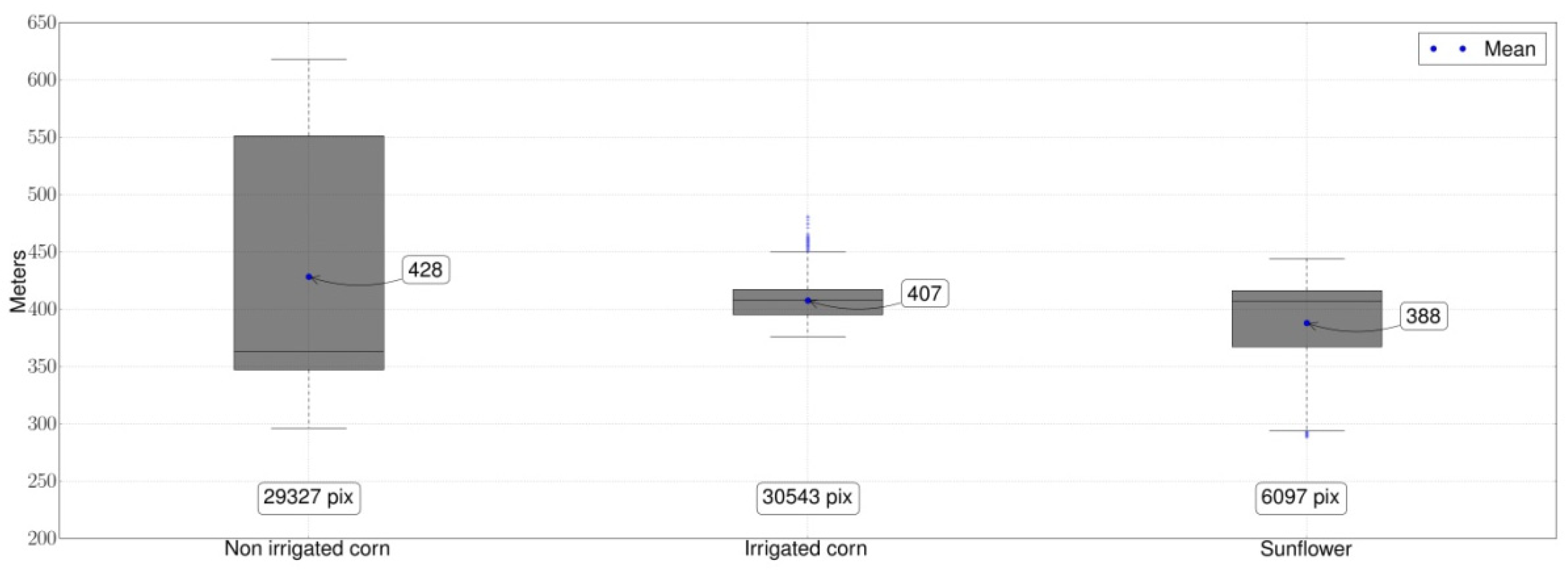
The reference dataset was established through three field campaigns carried out at different stages of the growing season: after sowing (May 2015), at flowering (July 2015), and during senescence (September 2015). Irrigated maize crops were identified by the presence of irrigation equipment or from information supplied directly by the farmer. The dataset was composed of 317 fields (114 irrigated maize and 203 non-irrigated fields: 171 growing maize and 32 sunflower) (Table 1). The irrigated plots covered more restricted elevations (Figure 2), and the mean size of the fields concerned was larger than for non-irrigated crops. The two irrigation systems most frequently used in our region are pitons and sprinkler systems. The plots equipped with piton systems are often larger and located on flat areas.

2.3. Landsat 8 Images

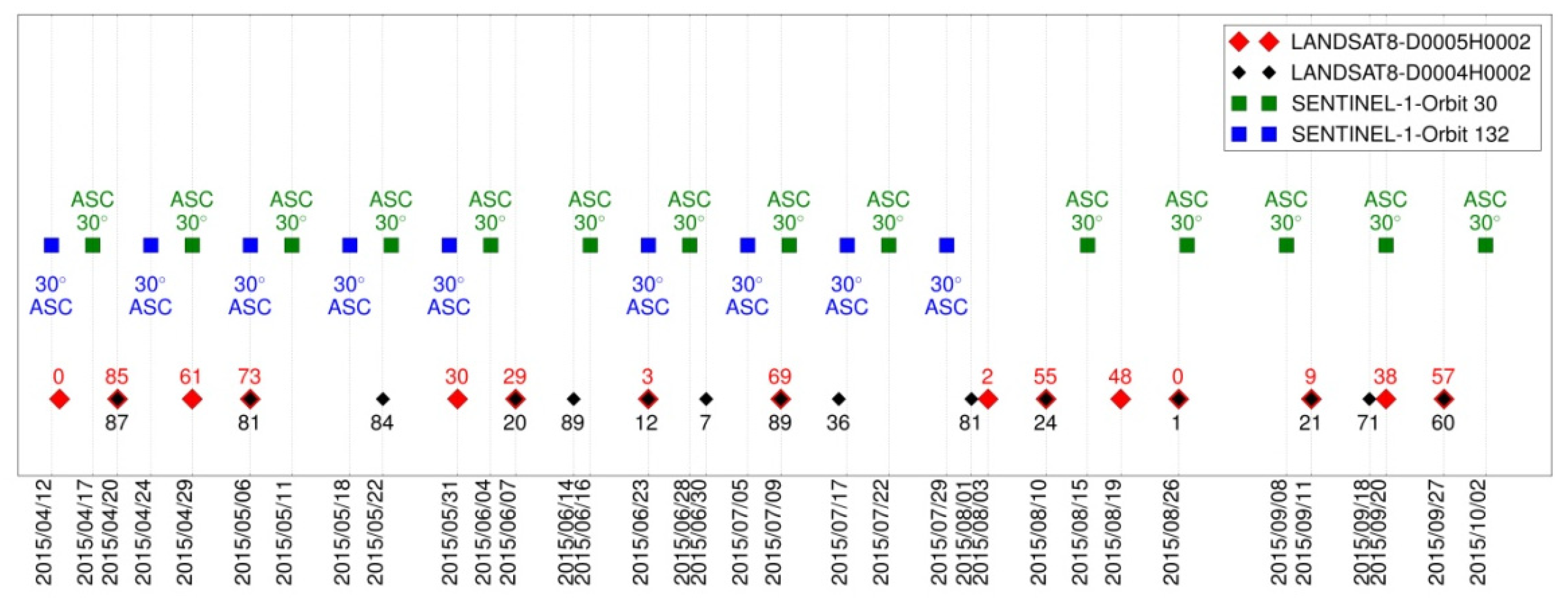
The Landsat 8 images were processed to level 2A (i.e., surface reflectance atmospherically corrected, with masks for clouds, cloud shadows, snow and water) as described in Hagolle [54]. Their acquisition dates, spatial resolution, incident, and viewing angles are listed in Figure 3. The number of cloudy pixels varied from 0.2% to 90% depending on the dates. For this study, we used the visible, near infrared, and short-wave infrared bands dedicated to vegetation surveys (482 nm, 561 nm, 654 nm, 864 nm, 1608 nm, 2200 nm).
The study site was covered by two Landsat 8 tiles (Figure 1). The images were resampled at 10 m in order to be merged with the SAR images as suggested by Inglada et al. [31].

2.4. SAR Images

The radar images came from the C-SAR instrument onboard the Sentinel-1A satellite (Interferometric Wide Swath mode). At the time of the study, the revisit time was 12 days. Revisit time has since improved (from three to six days) with the combination of S1-A and S1-B platforms.
This instrument supplies images at constant incidence angle in VV and VH polarization and with a 10 m spatial resolution along a 250 km swath. Images acquired at orbits 30 (12 images) and 132 (7 images) were used. All images were Level 1-GRD (Ground Range Detected), radiometrically corrected, filtered for speckle reduction using a Lee 3 by 3 filter [55], and orthorectified using the Sentinel-1 Toolbox (https://sentinel.esa.int/web/sentinel/toolboxes/sentinel-1). The dates of acquisitions, incident angles and orbits of the SAR images are listed in Figure 3. For both sensors, the geometric accuracy is estimated to be better than 30 m [31].

3. Method

3.1. Incremental Classification

We employed an incremental processing scheme to evaluate the usefulness of each date of acquisition and of each sensor for performing the seasonal classifications. For this purpose, we generated a supervised classification every time that a new image acquisition was available, using the previously available imagery. Every new acquisition led to a new classification.
A fully automated processing chain based on OpenCv 2.4 and GDAL 1.11 libraries was developed for this study. The classifier used was the Random Forest algorithm. The number of trees was set to 100, and the maximum depth to 25.
Temporal gap filling of the cloudy pixels was performed with the gap-filling module of the Iota2 software [21]. The method relies on a linear interpolation of the cloudy pixels using the previous and following cloud-free dates. The Landsat 8 images used in the classification process were thus gapfilled, providing one image every 16 days.
Every classification was evaluated using the reference dataset, which was randomly split into two parts: 50% of the ground truth polygons were used for training the classification and 50% were used for the validation. The global performance of each classification was evaluated using the Kappa coefficient (k) [56], and the performances of each class were evaluated using the F-score (Equation (1)), the precision (Equation (2)), and the recall metrics (Equation (3)).
F s c o r e =   2 × ( P i × R i ) P i + R i
P i = N u m b e r   o f   p i x e l s   o f   c l a s s   i   o f   t h e   r e f e r e n c e   d a t a s e t T o t a l     n u m b e r   o f   p i x e l s   i n   t h e   r e f e r e n c e   d a t a s e t
R i = N u m b e r   o f   p i x e l s   o f   c l a s s   i   i n   t h e   r e f e r e n c e   d a t a s e t T o t a l   n u m b e r   o f   p i x e l s   o f   c l a s s   i
As in the study by Inglada et al. [31], the random split was done 10 times in order to perform 10 classifications. This allowed the average and confidence intervals for the Kappa, Fscore, and recall to be computed.

3.2. Selected Features

Recent studies [21,25,31] have shown that the spectral reflectances, the Normalized Difference Vegetation Index (NDVI) [57], the Normalized Difference Water Index (NDWI) [58], and the Brightness Index [59] are sufficient to capture the main patterns of various crops observed with high spatial (optical) and temporal resolution imagery. We thus used these features to perform the optical classifications.
Since irrigated and non-irrigated crops tend to be cultivated at different elevation ranges (Figure 2), we decided to evaluate the impact of the Digital Elevation Model (DEM) on the classification procedure. The DEM used was the Shuttle Radar Topography Mission (SRTM) DEM with a spatial resolution of 30 m [60]. The topographic variables derived from the DEM were the elevation (m), the slope (°), and the aspect (°).
Inglada et al. [31] showed that the most pertinent features for crop classification performed with SAR imagery were the VV polarization, the Haralik textures (Entropy and Inertia computed from VV polarization), and the polarization ratio (VV/VH). In our study, we added the VH polarization and also the Entropy and the Inertia computed from the VH polarization. To evaluate the importance of these new additional features, we used the variable importance (VI) of the classifier [31,47]: in every tree grown in the forest, the out of bag samples were classified by using random permutations of each variable and computing the increase of classification errors with respect to the case without permutation. The median value of this number over all trees in the forest gave the importance score for each variable (VI). It was analysed for each classification.

3.3. Summer Crops Mask

A summer crops mask was produced from Landsat 8 images using the algorithm proposed by Marais-Sicre et al. [61]. It is based on a decision tree using multi-temporal NDVI thresholding. The classification algorithm is only applied over agricultural surfaces, previously extracted from the “Registre Parcellaire Graphique” provided by the French Services and Payment Agency.

4. Results and Discussion

4.1. Effect of Topographic Variables

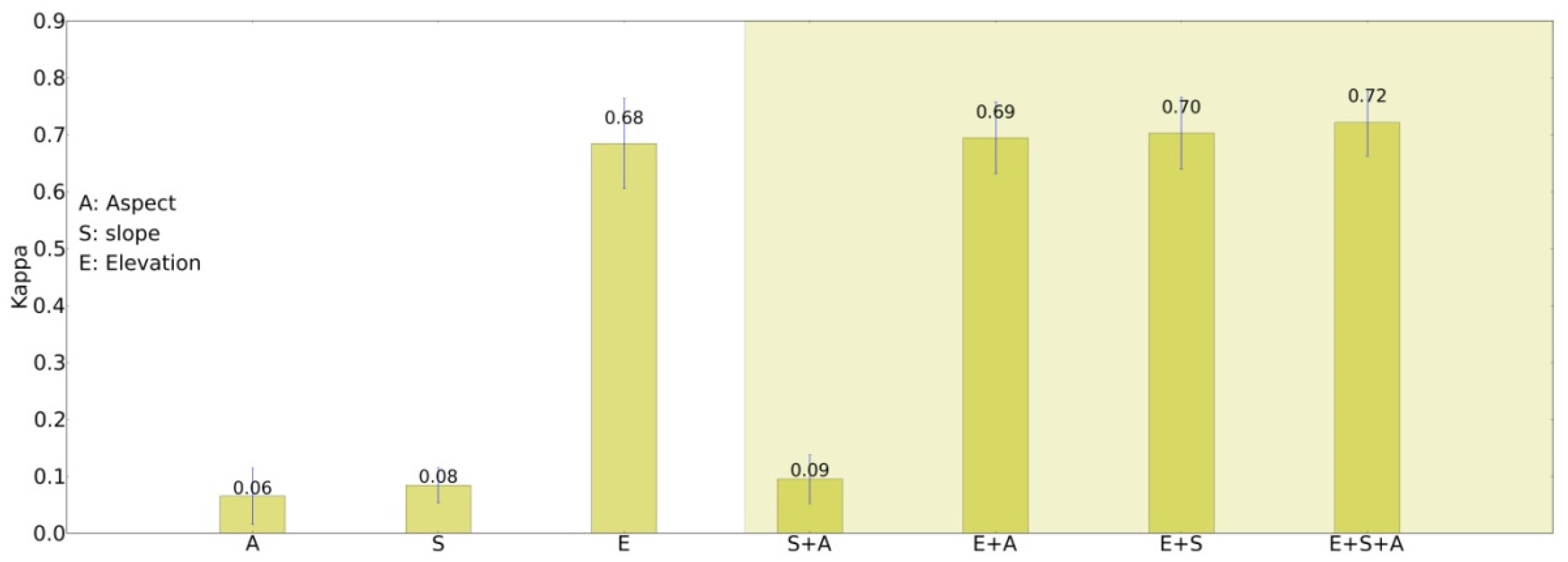
Figure 4 presents the k coefficient of the classification performed with the topographic variables only. Results reveal that, without the use of satellite imagery, the elevation feature alone enables irrigated and non-irrigated plots to be distinguished with k equal to 0.68. Slopes and aspects were not discriminant (0.06 < k < 0.08).
The elevation feature explains part of the variability existing between irrigated and non-irrigated crops as 90% of the irrigated surfaces are well classified (Table 2). However, confusion subsists as 46% of sunflower and 11% of non-irrigated maize pixels are classified as irrigated maize.

4.2. Incremental Classification Using Optical Images and Elevation Features

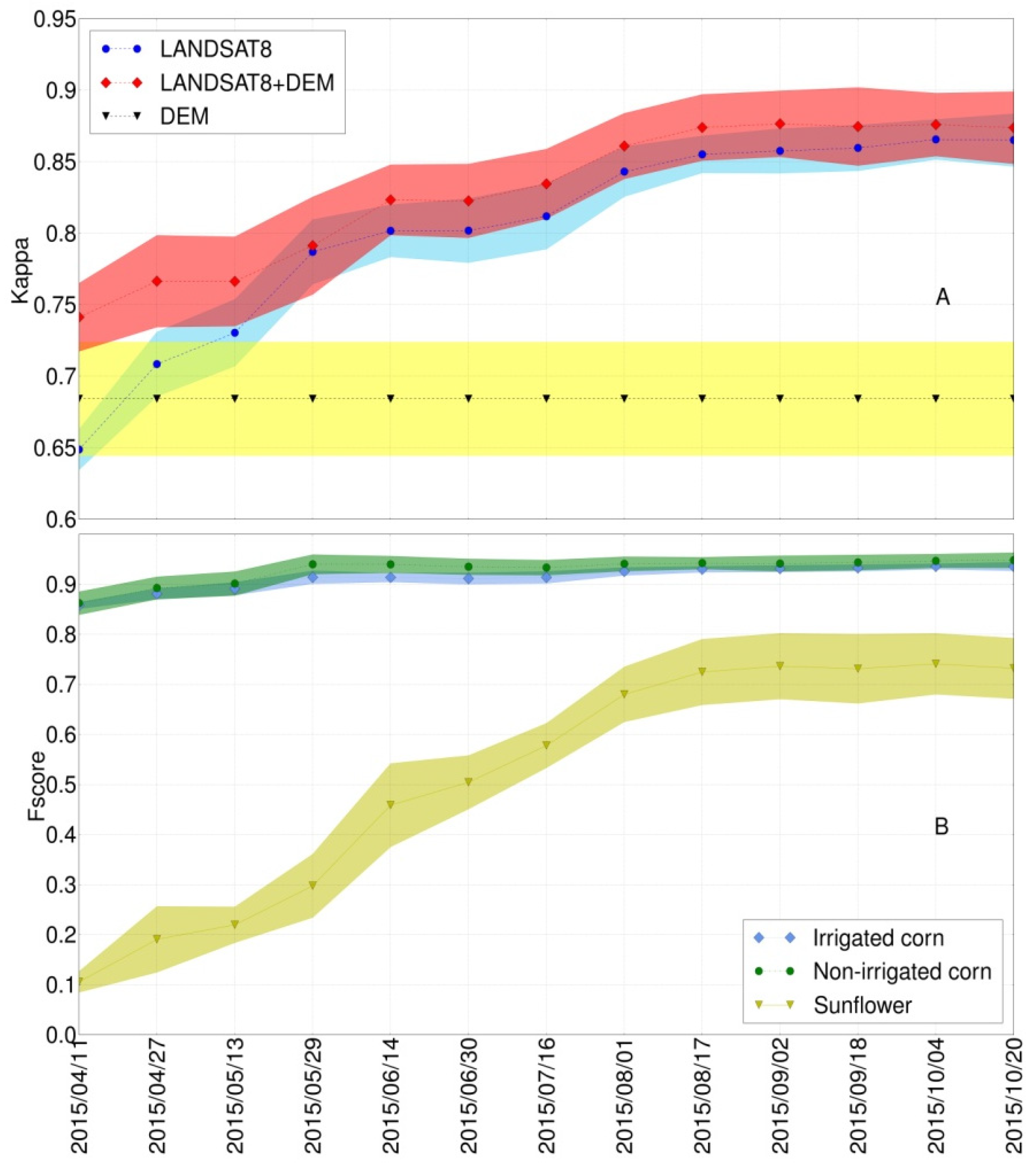
Figure 5 shows the evolution of k (Figure 5A) and Fscore (Figure 5B) of the incremental classifications for the following three scenarios:
(1)
with the elevation feature alone (Figure 5A, yellow curve);
(2)
with the spectral features of the Landsat 8 images listed in Section 3.2 (Figure 5A, blue curve); and
(3)
with both the elevation and optical imagery (Figure 5A, red curve).
In April, the k values vary between 0.65 (scenario 2) and 0.74 (scenario 3) with intermediate values (k = 0.68) for scenario 1. The addition of the elevation feature provides higher k values than are obtained with optical images alone. The gain due to elevation is significant at the beginning of the growing season, from April to mid-May, which is of major importance for early crop classification. During this period, the joint use of elevation and optical images (scenario 3) provides the highest k values. However, the gain due to the elevation feature decreases from June as the number of images increases. At the end of the season (before August), the k coefficients are similar for both scenarios (2 and 3), suggesting that DEM is not useful anymore.
The high k values from the start of the season hide strong disparities among the classes, with Fscores equal to 0.1 for sunflower and higher than 0.85 for maize (Figure 5B).
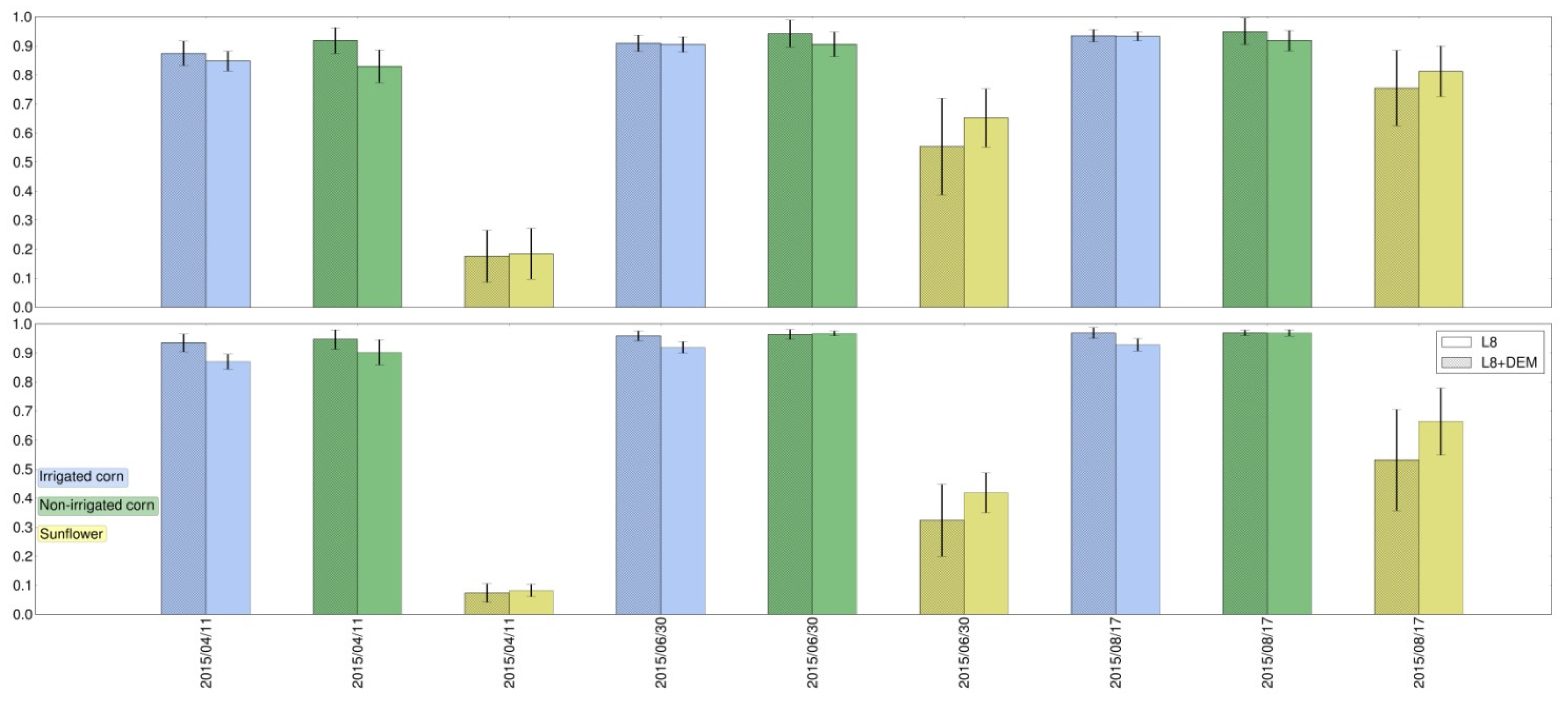
Analysis of the temporal evolution of the Fscore reveals that the increase of k observed until August is mainly due to a better classification of the sunflower crops. Figure 6 shows that the accuracy of the sunflower class was not improved by elevation, as precision and recall are decreased by the use of this feature. In contrast, maize classes (irrigated or not) are favourably influenced by elevation. The better identification of sunflower with additional optical images might be explained by the rapid growth of sunflower, making it easier to distinguish from maize. During this phase, the Fscores for maize (irrigated or non-irrigated) increases much less than those of sunflower.
From August to October, the period that corresponds to the maturity phases, k values for both scenarios (2 and 3) remain stable.

4.3. Incremental Classification Using Radar Images and Elevation

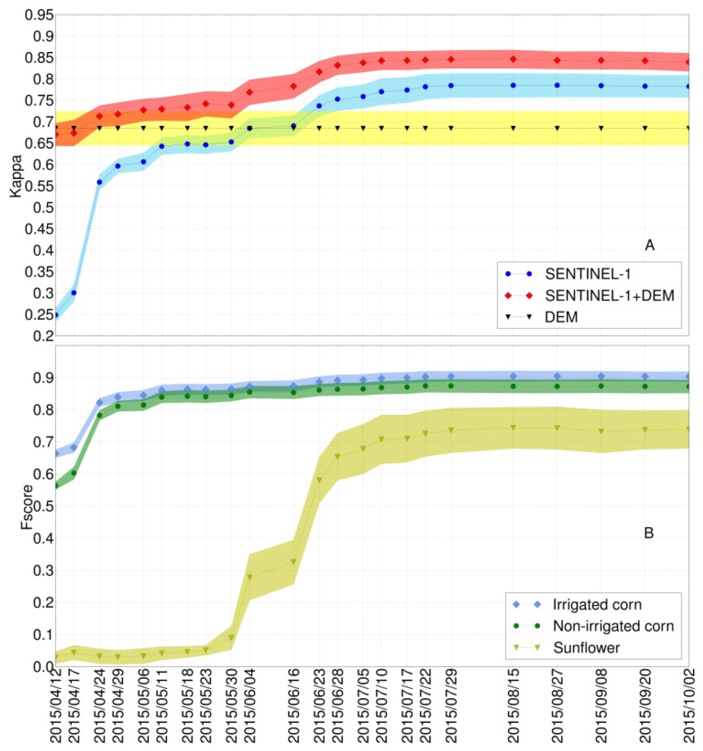
Figure 7 shows the evolution of k (Figure 7A) and Fscore (Figure 7B) of incremental classifications for the following three scenarios:
(1)
with the elevation feature only (Figure 7A, yellow curve);
(2)
with the radar features listed in Section 3.2 (Figure 7A, blue curve); and
(3)
with combined use of elevation and radar imagery (Figure 7A, red curve).
Unlike the results obtained with the optical images, those from radar data alone do not show good overall performance before late June (k = 0.75), when the plants are growing. These results show that, in our case study, the use of radar imagery alone is less accurate than optical imagery alone. Moreover, it is necessary to combine the SAR imagery with elevation (Figure 7A, scenario 3) to obtain performance comparable to that of optical imagery (Figure 5A). However, the performance observed in late June (Figure 7A, scenario 3) is reached about three weeks later than that using optical imagery with DEM (Figure 5A, scenario 3). This gain due to DEM is significant in the early season but becomes less significant in the end of the season.
The temporal analysis of kappa exhibits several phases:
  • In April (during sowing and emergence), the k coefficient of the radar classifications (scenario 2) increases significantly in connection with the Fscore increase for the irrigated and non-irrigated maize (Figure 7B). During this period, sunflower is very poorly classified (Fscore = 0.05) as plots correspond to bare soil mainly subjected to strong variations in moisture and roughness, to which the SAR signal is very sensitive.
  • From May to the end of June, k increases moderately, probably due to a better detection of sunflower, as shown by the increase in the Fscore of this class.
  • From July to October, gains in k and in Fscore are negligible. At this stage, all crops have reached their maximum development.
Whatever the phase, the irrigated maize class is characterized by higher Fscore values than the non-irrigated maize class. This result can be explained by the use of irrigation, which tends to spatially homogenize the crops, whereas non-irrigated maize exhibits larger spatial variations and is thus less easy to classify.
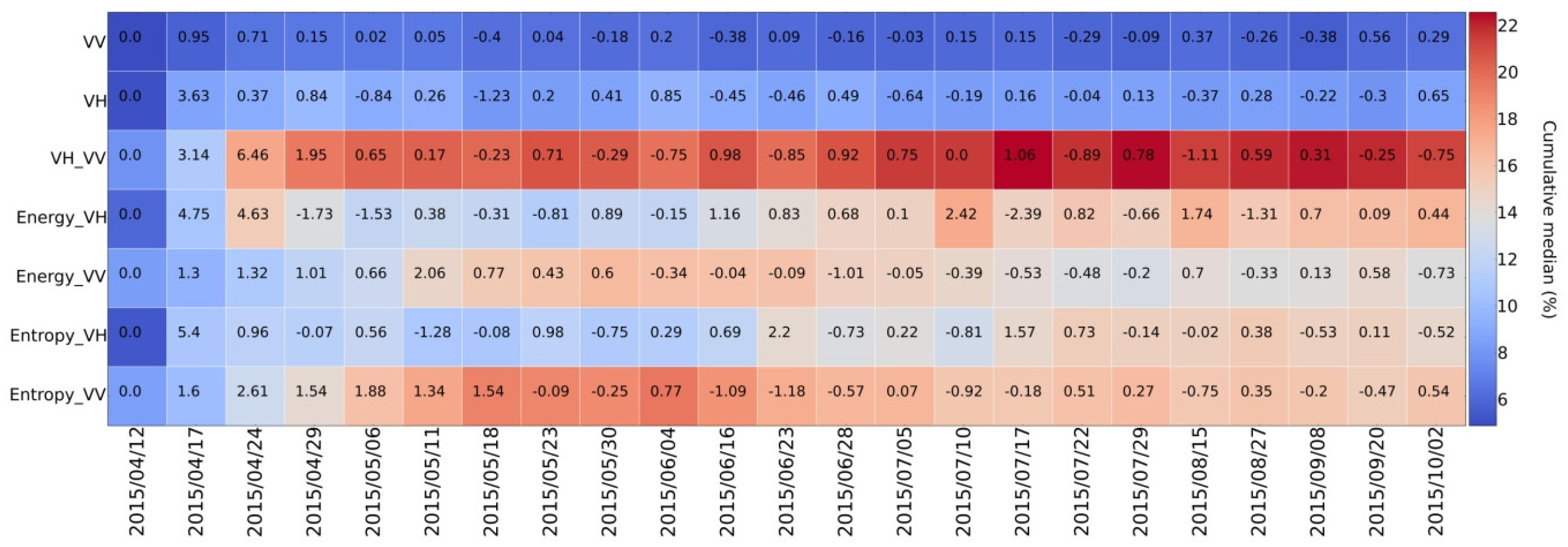
Figure 8 reveals that the most important features in the classification scheme are VH/VV ratio and Haralik textures. This result corroborates those of Inglada et al. [31]. There is a significant gain of the VI for VH/VV ratio and energy-VH between April 17 and April 24, when they reach 6.46 and 4.63, respectively. This gain explains the increase of the Fscore of maize classes observed during the same period (Figure 7B). Between mid-June and early July, we note successive gains of the VI for VH/VV ratio and energy-VH features. These gains are correlated with the increasing Fscore of Sunflower classes (Figure 7B). These primitives appear to be the most pertinent feature as they are more sensitive to crop architecture.

4.4. Multi-Temporal Classifications Using Optical and SAR Images

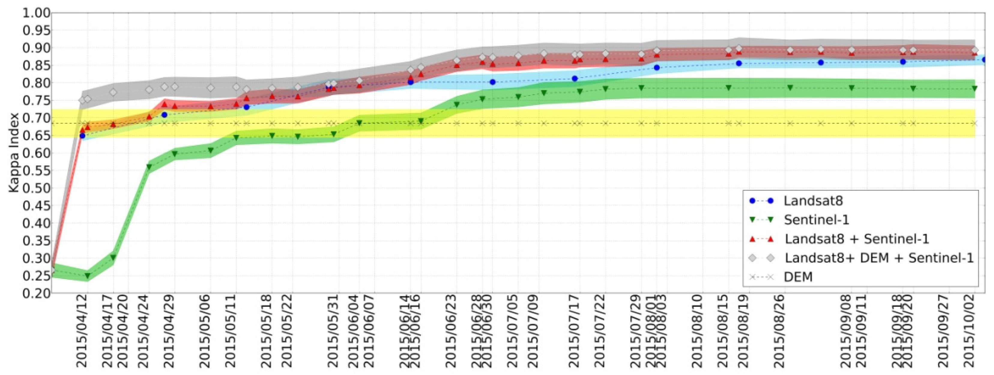
Figure 9 shows the evolution of k with time for the following five scenarios:
(1)
with the elevation (yellow curve);
(2)
with the optical images (blue curve);
(3)
with the radar images (green curve);
(4)
with optical and radar imagery (red curve); and
(5)
with optical and radar and elevation (grey curve).
Figure 9 shows that the combined use of radar and optical imagery (scenarios 4 and 5) leads to the best results (k = 0.89) throughout the whole season. The gain due to the elevation (scenario 5) is significant in the early season, from April to the end of May, and becomes negligible thereafter.
Between mid-June and the end of July, the combined use of optical and radar imagery leads to a k value significantly higher than those obtained with optical or radar imagery alone, which is of major importance for early crop detection. We also note that the performance of the optical classifications is higher than that of the radar classifications throughout the season.

5. Conclusions

In this paper, we investigate the usefulness of both radar and optical imagery combined with a digital elevation model to perform in-season classification of irrigated maize crops. The results reveal that the combined use of Sentinel-1 and Landsat 8 data improves the accuracy of the classifications with respect to those performed with optical or radar images alone. The gain is significant between April and the end of June, with k values increasing from 0.25 to 0.85 when the irrigation campaign starts, which is of major interest for water management. After this date, the gain in accuracy is less significant, with k values increasing slightly, from 0.85 to 0.9.
As in other studies [37,39,40], the elevation feature improves early classification until late May. After that, the gain becomes negligible.
Our results also reveal that Sentinel 1 images used alone do not perform early detection well and need to be combined with the elevation feature to reach performance similar to the combined use of optical data and DEM, but with a delay of three weeks.
However, the use of radar data is indispensable if we want to develop methods that are robust through time and over large zones as, unlike optical images, such data are not dependent on meteorological conditions. The use of radar data will also help to limit the use of temporal gap-filled optical data that could cause artefacts in the cloud masking algorithm and thus the classification process. As a follow on to this study, we intend to investigate the usefulness of Sentinel 2 data instead of Landsat 8, combined with Sentinel 1. We also plan to evaluate the usefulness of phenological indicators such as those put forward by Bargiel [62] and of meteorological data such as suggested by Peña-Arancibia et al. [41], which have been shown to significantly improve crop classifications for grasslands, maize, canola, sugar beets and potatoes.

Author Contributions

V.D., F.B. and F.H.: writing, methodology and analysis; F.H.: software; C.M.-S.: reference data.

Funding

This research was funded by the BPI, the FEDER and CASDAR funds in the framework of the MAISEO and the SIMULT’EAU projects.

Acknowledgments

The authors would like to thank Marjorie Battude for her valuable help in the field campaigns and Jerome Cros for his technical support.

Conflicts of Interest

The authors declare no conflict of interest.

References

  1. Loubier, S.; Campardon, M.; Morardet, S. L’irrigation diminue-t-elle en France? Premiers enseignements du recensement agricole de 2010. In Sciences Eaux & Territoires; IRSTEA: Villeurbanne, France, 2013. [Google Scholar]
  2. Bastiaanssen, W.G.M.; Molden, D.J.; Makin, I.W. Remote sensing for irrigated agriculture: Examples from research and possible applications. Agric. Water Manag. 2000, 46, 137–155. [Google Scholar] [CrossRef]
  3. Ozdogan, M.; Yang, Y.; Allez, G.; Cervantes, C. Remote Sensing of Irrigated Agriculture: Opportunities and Challenges. Remote Sens. 2010, 2, 2274–2304. [Google Scholar] [CrossRef] [Green Version]
  4. Goetz, S.J.; Varlyguin, D.; Smith, A.J.; Wright, R.K.; Prince, S.D.; Mazzacato, M.E.; Tringe, J.; Jantz, C.; Melchoir, B. Application of multitemporal Landsat data to map and monitor land cover and land use change in the Chesapeake Bay watershed. In Analysis of Multi-temporal Remote Sensing Images; World Scientific: Singapore, 2004. [Google Scholar]
  5. Knight, J.K.; Lunetta, R.L.; Ediriwickrema, J.; Khorram, S. Regional scale land-cover characterization using MODIS-NDVI 250 m multi-temporal imagery: A phenology based approach. Gisci. Remote Sens. 2006, 43, 1–23. [Google Scholar] [CrossRef]
  6. Velpuri, N.M.; Thenkabail, P.S.; Gumma, M.K.; Biradar, C.M.; Dheeravath, V.; Noojipady, P.; Yuanjie, L. Influence of Resolution in Irrigated Area Mapping and Area Estimations. Photogramm. Eng. Remote Sens. 2009, 75, 1383–1396. [Google Scholar] [CrossRef]
  7. Thenkabail, P.; Dheeravath, V.; Biradar, C.; Gangalakunta, O.R.; Noojipady, P.; Gurappa, C.; Velpuri, M.; Gumma, M.; Li, Y.; Thenkabail, P.S.; et al. Irrigated Area Maps and Statistics of India Using Remote Sensing and National Statistics. Remote Sens. 2009, 1, 50–67. [Google Scholar] [CrossRef] [Green Version]
  8. Dheeravath, V.; Thenkabail, P.S.; Chandrakantha, G.; Noojipady, P.; Reddy, G.P.O.; Biradar, C.M.; Gumma, M.K.; Velpuri, M. Irrigated areas of India derived using MODIS 500 m time series for the years 2001–2003. ISPRS J. Photogramm. Remote Sens. 2010, 65, 42–59. [Google Scholar] [CrossRef]
  9. Bouvet, A.; le Toan, T. Use of ENVISAT/ASAR wide-swath data for timely rice fields mapping in the Mekong River Delta. Remote Sens. Environ. 2011, 115, 1090–1101. [Google Scholar] [CrossRef] [Green Version]
  10. Gumma, M.K.; Thenkabail, P.S.; Maunahan, A.; Islam, S.; Nelson, E.A. Mapping seasonal rice cropland extent and area in the high cropping intensity environment of Bangladesh using MODIS 500 m data for the year 2010. ISPRS J. Photogramm. Remote Sens. 2014, 91, 98–113. [Google Scholar] [CrossRef]
  11. Zheng, B.; Myint, S.W.; Thenkabail, P.S.; Aggarwal, R.M. A support vector machine to identify irrigated crop types using time-series Landsat NDVI data. Int. J. Appl. Earth Obs. Geoinf. 2015, 34, 103–112. [Google Scholar] [CrossRef]
  12. Zhang, H.K.; Roy, D.P. Using the 500 m MODIS land cover product to derive a consistent continental scale 30 m Landsat land cover classification. Remote Sens. Environ. 2017, 197, 15–34. [Google Scholar] [CrossRef]
  13. Ouzemou, J.-E.; El Harti, A.; Lhissou, R.; El Moujahid, A.; Bouch, N.; El Ouazzani, R.; Bachaoui, E.M.; El Ghmari, A. Crop type mapping from pansharpened Landsat 8 NDVI data: A case of a highly fragmented and intensive agricultural system. Remote Sens. Appl. Soc. Environ. 2018, 11, 94–103. [Google Scholar] [CrossRef]
  14. Product User Guide, CCI LC PUGv2. Available online: http://maps.elie.ucl.ac.be/CCI/viewer/download/ESACCI-LC-Ph2-PUGv2_2.0.pdf (accessed on 30 July 2018).
  15. Torres, R.; Snoeij, P.; Geudtner, D.; Bibby, D.; Davidson, M.; Attema, E.; Potin, P.; Rommen, B.; Floury, N.; Brown, M.; et al. GMES Sentinel-1 mission. Remote Sens. Environ. Sentin. Mission. New Oppor. Sci. 2012, 120, 9–24. [Google Scholar] [CrossRef]
  16. Drusch, M.; Del Bello, U.; Carlier, S.; Colin, O.; Fernandez, V.; Gascon, F.; Hoersch, B.; Isola, C.; Laberinti, P.; Martimort, P.; et al. Sentinel-2: ESA’s Optical High-Resolution Mission for GMES Operational Services. Remote Sens. Environ. Sentin. Mission. New Oppor. Sci. 2012, 120, 25–36. [Google Scholar] [CrossRef]
  17. Ozdogan, M.; Gutman, G. A new methodology to map irrigated areas using multi-temporal MODIS and ancillary data: An application example in the continental US. Remote Sens. Environ. 2008, 112, 3520–3537. [Google Scholar] [CrossRef] [Green Version]
  18. Julien, Y.; Sobrino, J.A.; Jiménez-Muñoz, J.-C. Land use classification from multitemporal Landsat imagery using the Yearly Land Cover Dynamics (YLCD) method. Int. J. Appl. Earth Obs. Geoinf. 2011, 13, 711–720. [Google Scholar] [CrossRef]
  19. Miao, X.; Heaton, J.S.; Zheng, S.; Charlet, D.A.; Liu, D.H. Applying tree-based ensemble algorithms to the classification of ecological zones using multi-temporal multi-source remote-sensing data. Int. J. Remote Sens. 2012, 33, 1823–1849. [Google Scholar] [CrossRef]
  20. Valero, S.; Morin, D.; Inglada, J.; Sepulcre, G.; Arias, M.; Hagolle, O.; Dedieu, G.; Bontemps, S.; Defourny, P. Processing Sentinel-2 image time series for developing a real-time cropland mask. In Proceedings of the 2015 IEEE International Geoscience and Remote Sensing Symposium (IGARSS), Milan, Italy, 26–30 July 2015; pp. 2731–2734. [Google Scholar] [CrossRef]
  21. Inglada, J.; Arias, M.; Tardy, B.; Hagolle, O.; Valero, S.; Morin, D.; Dedieu, G.; Sepulcre, G.; Bontemps, S.; Defourny, P.; et al. Assessment of an Operational System for Crop Type Map Production Using High Temporal and Spatial Resolution Satellite Optical Imagery. Remote Sens. 2015, 7, 12356–12379. [Google Scholar] [CrossRef] [Green Version]
  22. Valero, S.; Morin, D.; Inglada, J.; Sepulcre, G.; Arias, M.; Hagolle, O.; Dedieu, G.; Bontemps, S.; Defourny, P.; Koetz, B.; et al. Production of a Dynamic Cropland Mask by Processing Remote Sensing Image Series at High Temporal and Spatial Resolutions. Remote Sens. 2016, 8, 55. [Google Scholar] [CrossRef]
  23. Immitzer, M.; Vuolo, F.; Atzberger, C.; Immitzer, M.; Vuolo, F.; Atzberger, E.C. First Experience with Sentinel-2 Data for Crop and Tree Species Classifications in Central Europe. Remote Sens. 2016, 8, 166. [Google Scholar] [CrossRef]
  24. Asgarian, A.; Soffianian, A.; Pourmanafi, S. Crop type mapping in a highly fragmented and heterogeneous agricultural landscape: A case of central Iran using multi-temporal Landsat 8 imagery. Comput. Electron. Agric. 2016, 127, 531–540. [Google Scholar] [CrossRef]
  25. Pelletier, C.; Valero, S.; Inglada, J.; Champion, N.; Dedieu, G. Assessing the robustness of Random Forests to map land cover with high resolution satellite image time series over large areas. Remote Sens. Environ. 2016, 187, 156–168. [Google Scholar] [CrossRef]
  26. Pelletier, C.; Valero, S.; Inglada, J.; Champion, N.; Marais Sicre, C.; Dedieu, G.; Pelletier, C.; Valero, S.; Inglada, J.; Champion, N.; et al. Effect of Training Class Label Noise on Classification Performances for Land Cover Mapping with Satellite Image Time Series. Remote Sens. 2017, 9, 173. [Google Scholar] [CrossRef]
  27. Moody, D.I.; Brumby, S.P.; Chartrand, R.; Keisler, R.; Longbotham, N.; Mertes, C.; Skillman, S.W.; Warren, M.S. Crop classification using temporal stacks of multispectral satellite imagery. In Proceedings of the Algorithms and Technologies for Multispectral, Hyperspectral, and Ultraspectral Imagery XXIII, Anaheim, CA, USA, 9–13 April 2017; p. 101980G. [Google Scholar] [CrossRef]
  28. Sonobe, R.; Yamaya, Y.; Tani, H.; Wang, X.; Kobayashi, N.; Mochizuki, K. Crop classification from Sentinel-2-derived vegetation indices using ensemble learning. J. Appl. Remote Sens. 2018, 12, 026019. [Google Scholar] [CrossRef]
  29. Vuolo, F.; Neuwirth, M.; Immitzer, M.; Atzberger, C.; Ng, W.-T. How much does multi-temporal Sentinel-2 data improve crop type classification? Int. J. Appl. Earth Obs. Geoinf. 2018, 72, 122–130. [Google Scholar] [CrossRef]
  30. Belgiu, M.; Csillik, E.O. Sentinel-2 cropland mapping using pixel-based and object-based time-weighted dynamic time warping analysis. Remote Sens. Environ. 2018, 204, 509–523. [Google Scholar] [CrossRef]
  31. Inglada, J.; Vincent, A.; Arias, M.; Marais-Sicre, C. Improved Early Crop Type Identification by Joint Use of High Temporal Resolution SAR and Optical Image Time Series. Remote Sens. 2016, 8, 362. [Google Scholar] [CrossRef]
  32. Sonobe, R.; Yamaya, Y.; Tani, H.; Wang, X.; Kobayashi, N.; Mochizuki, K. Assessing the suitability of data from Sentinel-1A and 2A for crop classification. Gisci. Remote Sens. 2017, 54, 918–938. [Google Scholar] [CrossRef]
  33. Yang, H.; Pan, B.; Wu, W.; Tai, J. Field-based rice classification in Wuhua county through integration of multi-temporal Sentinel-1A and Landsat-8 OLI data. Int. J. Appl. Earth Obs. Geoinf. 2018, 69, 226–236. [Google Scholar] [CrossRef]
  34. Whyte, A.; Ferentinos, K.P.; Petropoulos, G.P. A new synergistic approach for monitoring wetlands using Sentinels-1 and 2 data with object-based machine learning algorithms. Environ. Model. Softw. 2018, 104, 40–54. [Google Scholar] [CrossRef]
  35. Simonneaux, V.; Duchemin, B.; Helson, D.; Raki, E.; Olioso, A.; Chehbouni, A. The use of high-resolution image time series for crop classification and evapotranspiration estimate over an irrigated area in central Morocco. Int. J. Remote Sens. 2008, 29, 95–116. [Google Scholar] [CrossRef]
  36. Gumma, M.K.; Thenkabail, P.S.; Muralikrishna, I.V.; Velpuri, M.N.; Gangadhararao, P.T.; Dheeravath, V.; Biradar, C.M.; Nalan, S.A.; Gaur, A. Changes in agricultural cropland areas between a water-surplus year and a water-deficit year impacting food security, determined using MODIS 250 m time-series data and spectral matching techniques, in the Krishna River basin (India). Int. J. Remote Sens. 2011, 32, 3495–3520. [Google Scholar] [CrossRef]
  37. Edlinger, J.; Conrad, C.; Lamers, J.; Khasankhanova, G.; Koellner, T.; Edlinger, J.; Conrad, C.; Lamers, J.P.A.; Khasankhanova, G.; Koellner, T. Reconstructing the Spatio-Temporal Development of Irrigation Systems in Uzbekistan Using Landsat Time Series. Remote Sens. 2012, 4, 3972–3994. [Google Scholar] [CrossRef] [Green Version]
  38. Salmon, J.M.; Friedl, M.A.; Frolking, S.; Wisser, D.; Douglas, E.E.M. Global rain-fed, irrigated, and paddy croplands: A new high resolution map derived from remote sensing, crop inventories and climate data. Int. J. Appl. Earth Obs. Geoinf. 2015, 38, 321–334. [Google Scholar] [CrossRef]
  39. Ambika, A.K.; Wardlow, B.; Mishra, V. Remotely sensed high resolution irrigated area mapping in India for 2000 to 2015. Sci. Data 2016, 3, 160118. [Google Scholar] [CrossRef] [PubMed] [Green Version]
  40. Pervez, M.S.; Budde, M.; Rowland, J. Mapping irrigated areas in Afghanistan over the past decade using MODIS NDVI. Remote Sens. Environ. 2014, 149, 155–165. [Google Scholar] [CrossRef] [Green Version]
  41. Peña-Arancibia, J.L.; McVicar, T.R.; Paydar, Z.; Li, L.; Guerschman, J.P.; Donohue, R.J.; Dutta, D.; Podger, G.M.; van Dijk, A.I.J.M.; Chiew, F.H.S. Dynamic identification of summer cropping irrigated areas in a large basin experiencing extreme climatic variability. Remote Sens. Environ. 2014, 154, 139–152. [Google Scholar] [CrossRef]
  42. Conrad, C.; Löw, F.; Lamers, J.P.A. Mapping and assessing crop diversity in the irrigated Fergana Valley, Uzbekistan. Appl. Geogr. 2017, 86, 102–117. [Google Scholar] [CrossRef]
  43. Ferrant, S.; Selles, A.; Le Page, M.; Herrault, P.-A.; Pelletier, C.; Al-Bitar, A.; Mermoz, S.; Gascoin, S.; Bouvet, A.; Saqalli, M.; et al. Detection of Irrigated Crops from Sentinel-1 and Sentinel-2 Data to Estimate Seasonal Groundwater Use in South India. Remote Sens. 2017, 9, 1119. [Google Scholar] [CrossRef]
  44. Breiman, L. Random Forests. Mach. Learn. 2001, 45, 5–32. [Google Scholar] [CrossRef] [Green Version]
  45. Ho, T.K. The random subspace method for constructing decision forests. IEEE Trans. Pattern Anal. Mach. Intell. 1998, 20, 832–844. [Google Scholar]
  46. Ok, A.O.; Akar, O.; Gungor, O. Evaluation of random forest method for agricultural crop classification. Eur. J. Remote Sens. 2012, 45, 421–432. [Google Scholar] [CrossRef]
  47. Ghimire, B.; Rogan, J.; Rodriguez Galiano, V.; Panday, P.; Neeti, N. An evaluation of bagging, boosting, and Random Forests for land-cover classification in Cape Cod, Massachusetts, USA. Geosci. Remote Sens. 2012, 49, 623–643. [Google Scholar] [CrossRef]
  48. Rodriguez-Galiano, V.F.; Ghimire, B.; Rogan, J.; Chica-Olmo, M.; Rigol-Sanchez, E.J.P. An assessment of the effectiveness of a random forest classifier for land-cover classification. ISPRS J. Photogramm. Remote Sens. 2012, 67, 93–104. [Google Scholar] [CrossRef]
  49. Hao, P.; Wang, L.; Niu, Z. Comparison of Hybrid Classifiers for Crop Classification Using Normalized Difference Vegetation Index Time Series: A Case Study for Major Crops in North Xinjiang, China. PLoS ONE 2015, 10, e0137748. [Google Scholar] [CrossRef] [PubMed]
  50. Belgiu, M.; Drăguţ, L. Random forest in remote sensing: A review of applications and future directions. ISPRS J. Photogramm. Remote Sens. 2016, 114, 24–31. [Google Scholar] [CrossRef]
  51. Song, Q.; Hu, Q.; Zhou, Q.; Hovis, C.; Xiang, M.; Tang, H.; Wu, W.; Song, Q.; Hu, Q.; Zhou, Q.; et al. In-Season Crop Mapping with GF-1/WFV Data by Combining Object-Based Image Analysis and Random Forest. Remote Sens. 2017, 9, 1184. [Google Scholar] [CrossRef]
  52. Gao, Q.; Zribi, M.; Escorihuela, M.; Baghdadi, N.; Segui, P.; Gao, Q.; Zribi, M.; Escorihuela, M.J.; Baghdadi, N.; Segui, P.Q. Irrigation Mapping Using Sentinel-1 Time Series at Field Scale. Remote Sens. 2018, 10, 1495. [Google Scholar] [CrossRef]
  53. Battude, M.; Al Bitar, A.; Brut, A.; Tallec, T.; Huc, M.; Cros, J.; Weber, J.; Lhuissier, L.; Simonneaux, V.; Demarez, V. Modeling water needs and total irrigation depths of maize crop in the south west of France using high spatial and temporal resolution satellite imagery. Agric. Water Manag. 2017, 189, 123–136. [Google Scholar] [CrossRef]
  54. Hagolle, O.; Sylvander, S.; Huc, M.; Claverie, M.; Clesse, D.; Dechoz, C.; Lonjou, V.; Poulain, V. SPOT-4 (Take 5): Simulation of Sentinel-2 time series on 45 large sites. Remote Sens. 2015, 7, 12242–12264. [Google Scholar] [CrossRef]
  55. Lee, J.-S. Speckle Suppression and Analysis for Synthetic Aperture Radar Images. Opt. Eng. 1986, 25, 255636. [Google Scholar] [CrossRef]
  56. Congalton, R. A Review of Assessing the Accuracy of Classifications of Remotely Sensed Data. Remote Sens. Environ. 1991, 37, 35–46. [Google Scholar] [CrossRef]
  57. Tucker, C.J. Red and photographic infrared linear combinations for monitoring vegetation. Remote Sens. Environ. 1979, 8, 127–150. [Google Scholar] [CrossRef] [Green Version]
  58. Gao, B. NDWI—A normalized difference water index for remote sensing of vegetation liquid water from space. Remote Sens. Environ. 1996, 58, 257–266. [Google Scholar] [CrossRef]
  59. Caloz, R.; Abednego, B.; Collet, C. The Normalisation of a Soil Brightness Index for the Study of Changes in Soil Conditions. In Proceedings of the Spectral Signatures of Objects in Remote Sensing, Aussois, France, 18–22 January 1988; ESA SP-287. Guyenne, T.D., Hunt, J.J., Eds.; European Space Agency: Paris, France, 1988; p. 363. [Google Scholar]
  60. Abrams, M.; Bailey, B.; Tsu, H.; Hato, M. The ASTER global DEM. Photogramm. Eng. Remote Sens. 2010, 76, 344–348. [Google Scholar]
  61. Marais Sicre, C.; Inglada, J.; Fieuzal, R.; Baup, F.; Valero, S.; Cros, J.; Huc, M.; Demarez, V.; Marais Sicre, C.; Inglada, J.; et al. Early Detection of Summer Crops Using High Spatial Resolution Optical Image Time Series. Remote Sens. 2016, 8, 591. [Google Scholar] [CrossRef]
  62. Bargiel, D. A new method for crop classification combining time series of radar images and crop phenology information. Remote Sens. Environ. 2017, 198, 369–383. [Google Scholar] [CrossRef]
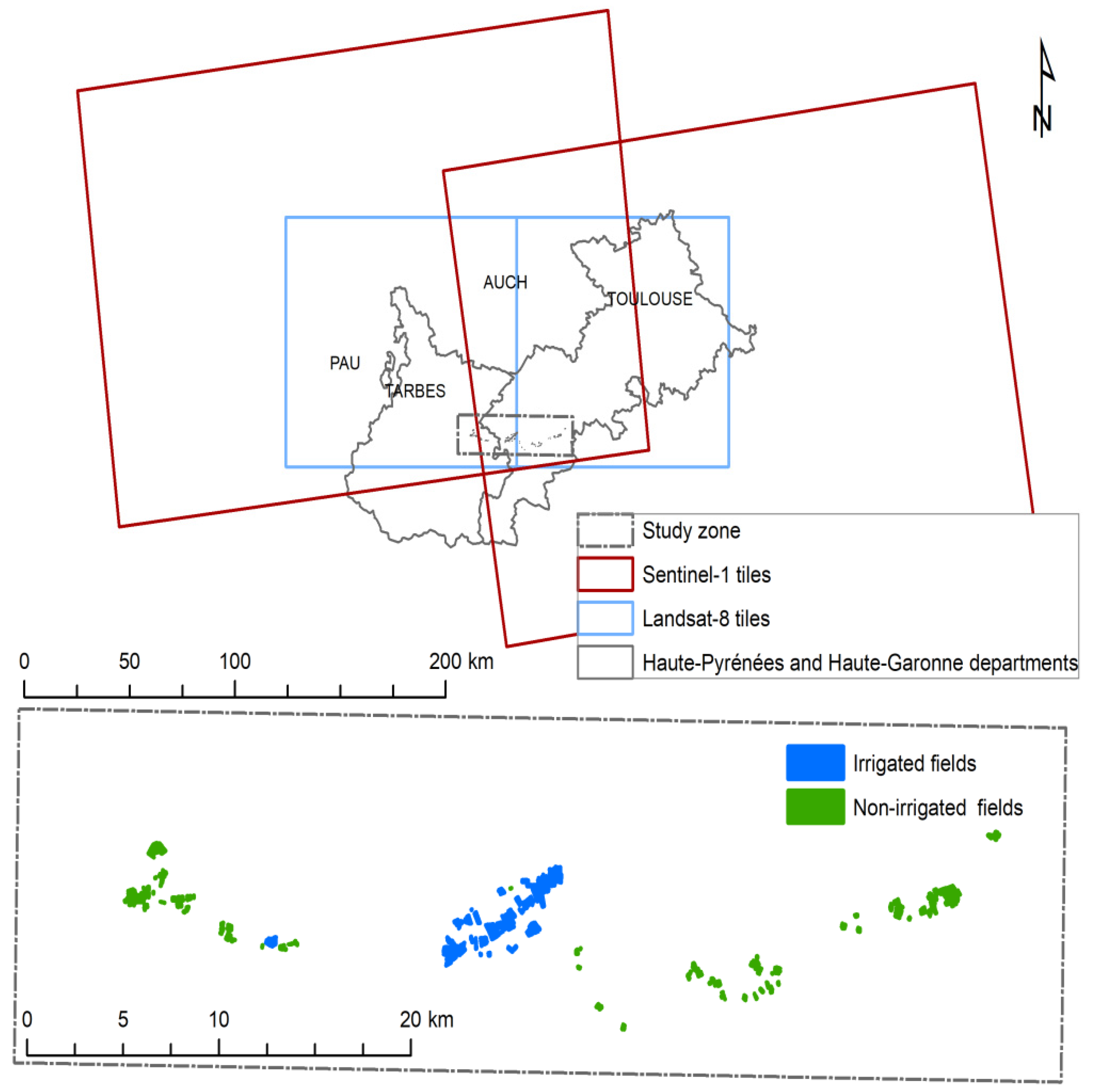
Figure 1. Location of the study zone with footprints of the Landsat-8 and Sentinel-1 images (top map) and field data (bottom map).
Remotesensing 11 00118 g001
Figure 2. Statistical distribution of elevations per class. The number of pixels per class is mentioned beside each boxplot.
Remotesensing 11 00118 g002
Figure 3. Time series of Landsat 8 images with cloud cover expressed in percent (red and black numbers) and Synthetic Aperture Radar (SAR)images with incidence angle expressed in degrees (green and blue numbers). ASC stands for ASCENDING orbit.
Remotesensing 11 00118 g003
Figure 4. k coefficient using Digital Elevation Model (DEM) features alone (aspect, slope, elevation, and their combined use). Error bars indicate 95% confidence intervals.
Remotesensing 11 00118 g004
Figure 5. Evolution of the Kappa coefficients (A) with time, with 95% confidence intervals, for the 3 scenarios. The Fscore is given for scenario 3 only (B)
Remotesensing 11 00118 g005
Figure 6. Precision (top) and recall metrics (bottom) for scenarios 2 and 3 for 14 April, 30 June, and 17 August.
Remotesensing 11 00118 g006
Figure 7. Temporal evolution of the k (A) and Fscore (scenario 3) (B) of the incremental classification with 95% confidence intervals for the three scenarios using elevation and radar imagery.
Remotesensing 11 00118 g007
Figure 8. Median of the Variable Importance cumulated for each SAR classification (legend bar). The number over each cell corresponds to the difference between the medians of two successive classifications.
Remotesensing 11 00118 g008
Figure 9. Temporal evolution of Kappa and Fscore coefficients of the incremental classification with 95% confidence intervals for the five scenarios.
Remotesensing 11 00118 g009
Table 1. Reference dataset.
Class LabelNumber of Fields SampledTotal Area Sampled (ha)Mean Field Size (ha)
Irrigated maize11425812.2
Non-irrigated maize17123721.3
Sunflower325051.5
Table 2. Confusion matrix using elevation alone. k = 0.68. Predicted classes are in columns and reference data are in rows.
Class LabelIrrigated MaizeNon-Irrigated MaizeSunflower
Irrigated maize90.380.389.24
Non-irrigated maize11.3587.121.22
Sunflower46.0614.3741.3