Flood Mapping with Convolutional Neural Networks Using Spatio-Contextual Pixel Information
Abstract
:1. Introduction
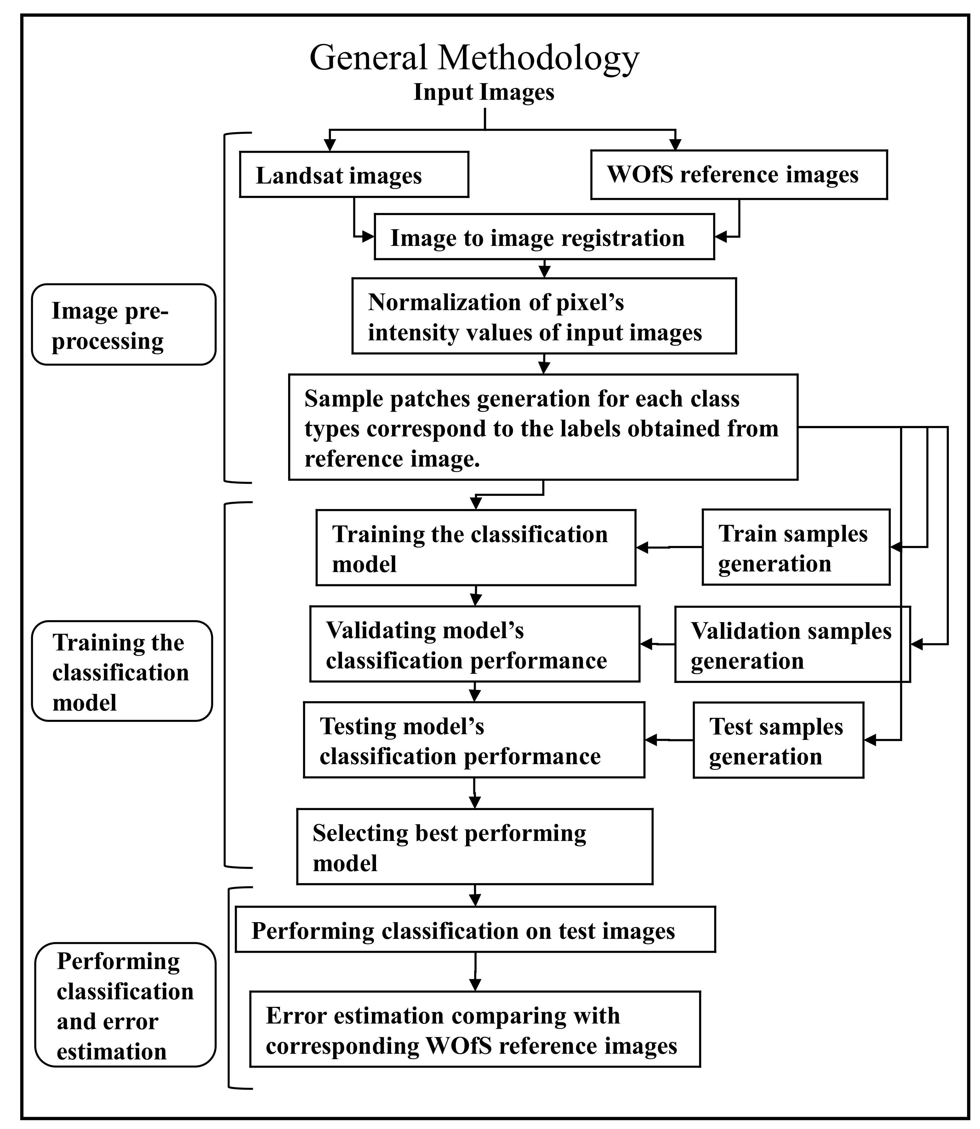
2. Methodology and Data Processing
2.1. Stage 1: Image Pre-Processing
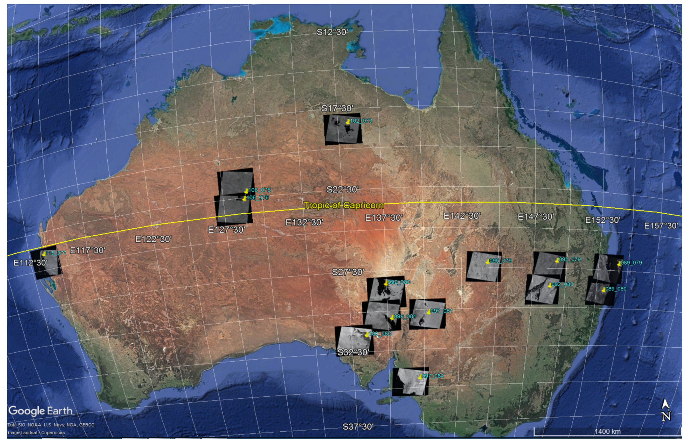
2.1.1. Landsat Data Collection
2.1.2. WOfS Reference Data Collection
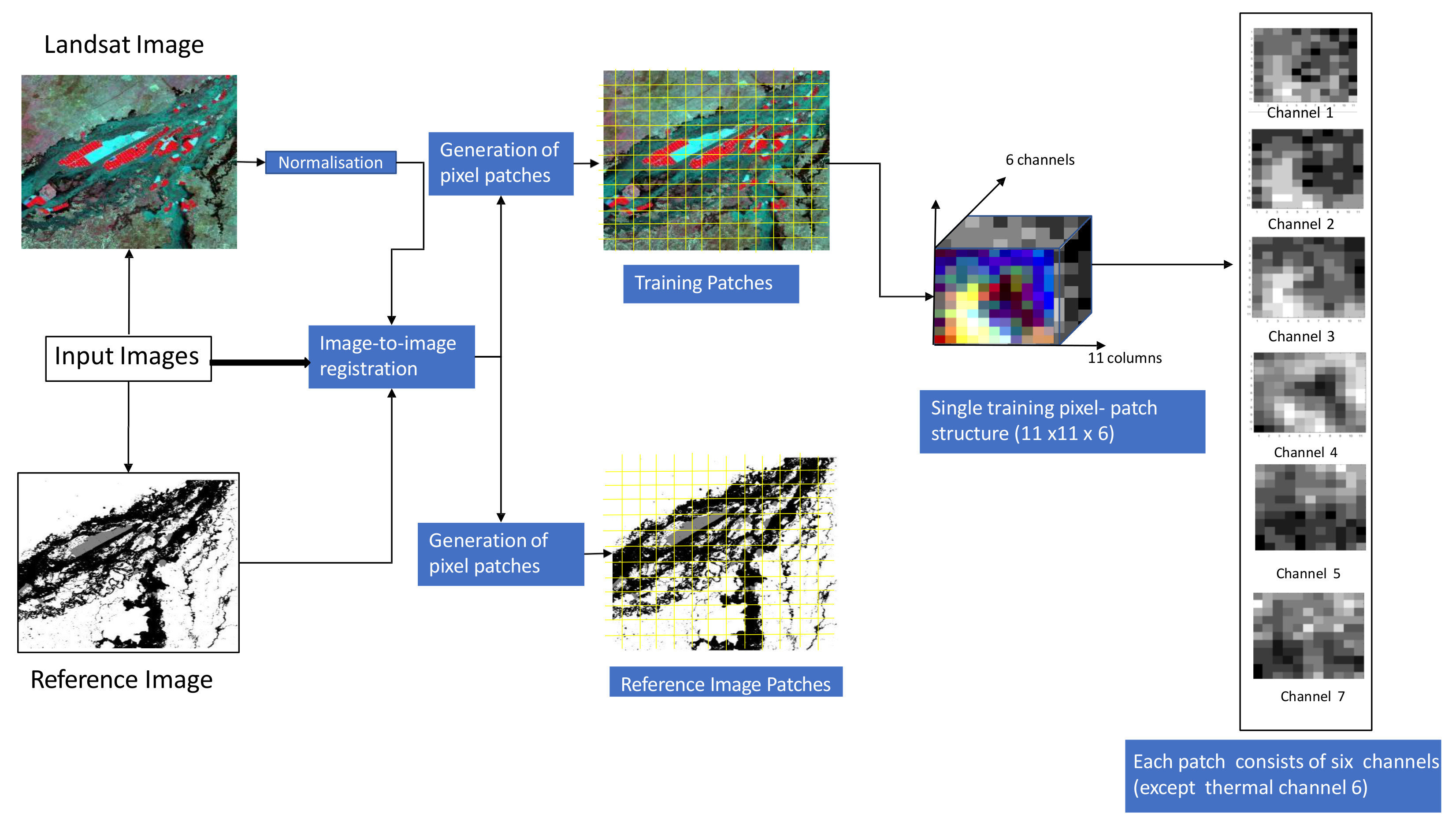
2.1.3. Image Registration
2.1.4. Data Normalization
2.1.5. Train, Validation and Test Sample Patches Generation for Model Design
2.2. Stage 2: Model Building and Training
2.2.1. Deep Network Structure
2.2.2. Training and Testing during Model Design
2.2.3. Validation during Model Design
2.2.4. Selecting Best Performing Model
2.3. Stage 3: Performing Classification and Error Estimation
3. Results
3.1. Training, Validation and Test Performances during the Model Design
- (1)
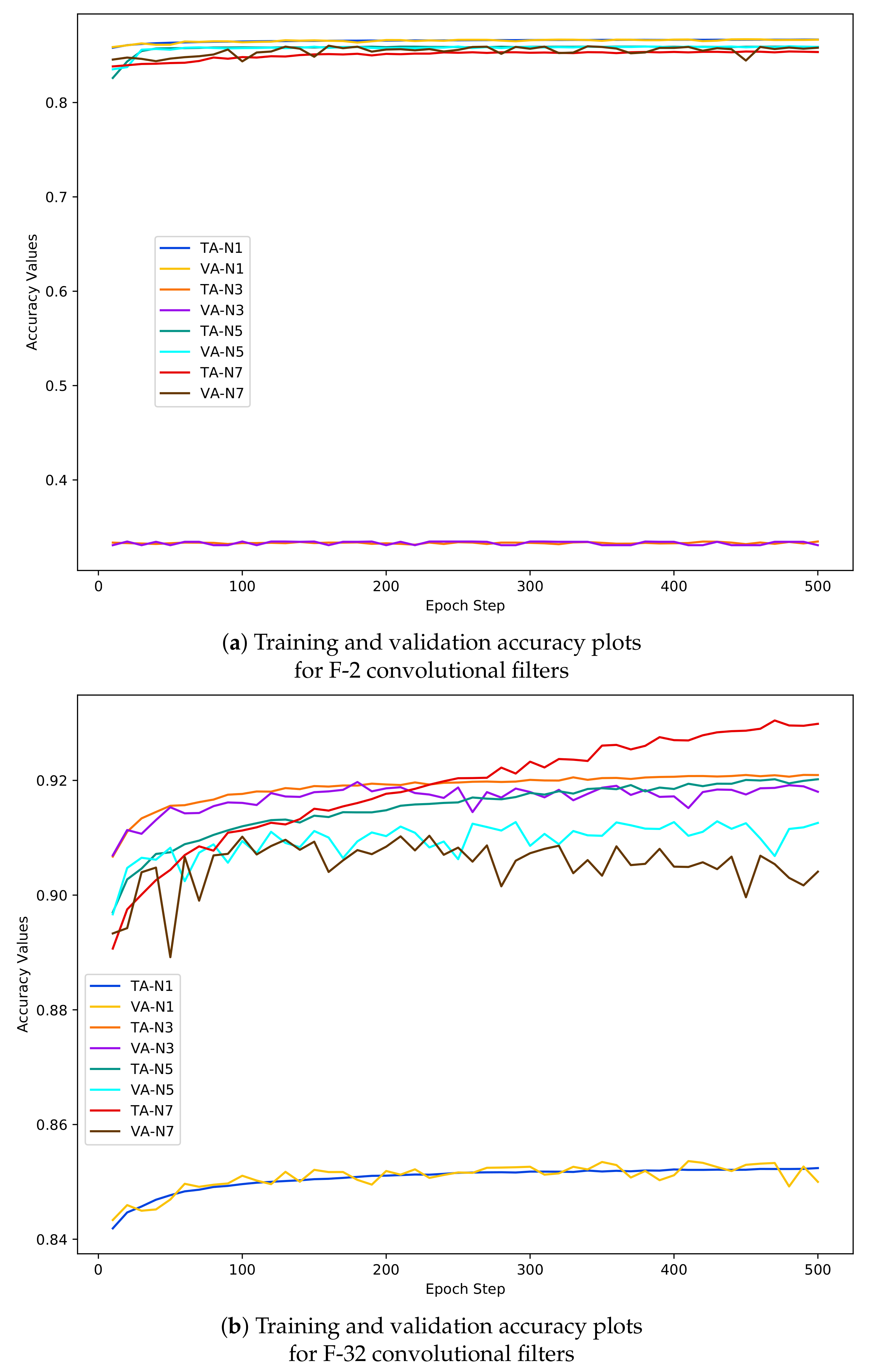
- N-1 training samples are the representative of pixel-wise training samples and the graphs exhibit highest accuracy (80%) of the model on training and validation data using N-1 training samples with 2 learnable filters in the convolutional layers (the yellow and blue coloured curves in Figure 7a). Increase in the number of learnable convolutional filters results decrease in model’s accuracy of the model using N-1 data.
- (2)
- Graphs in Figure 7b shows that the model’s performance improves drastically with the highest level of accuracy increases to 92% using 32 learnable filters. But the overall performance of the F-CNNs model using N-1 sample set increases from 80% but compared to the performance of N-3, N-5 and N-7, moves down to the lowest accuracy (84%) level.
- (3)
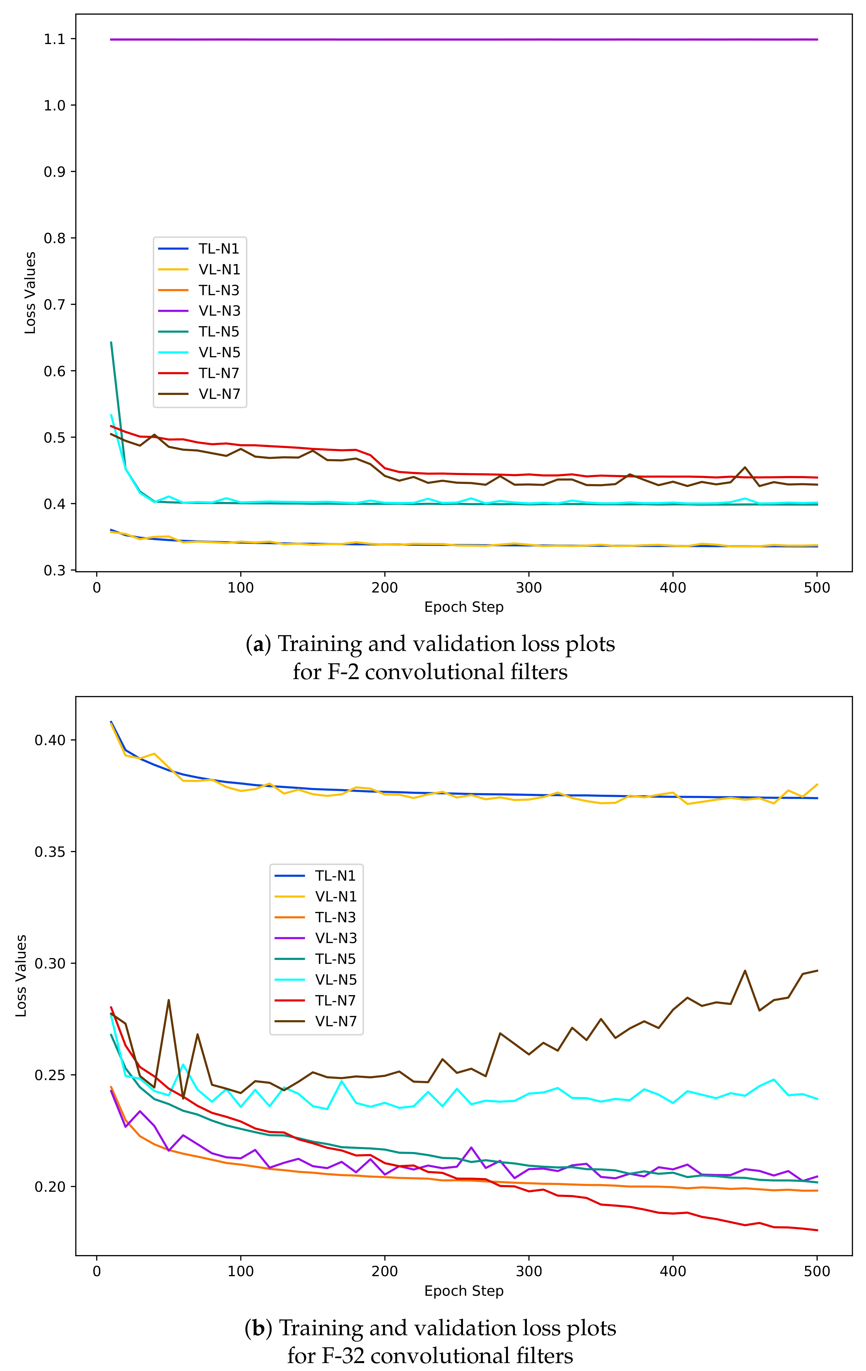
- The graphs in Figure 8 shows that the range of loss value remains constant (0.40–0.35) for N-1 training and validation data and the increase in filter numbers does not have any effect.
- (4)
- From the accuracy and loss graphs it can be outlined that the model performed with highest accuracy (95%) and lowest loss (0.20) values with N-3 samples (orange and violet coloured graph).
- (5)
- The F-CNNs model does not achieve the highest validation accuracy with N-5 and N-7 dastasets as we can see a deterioration of model’s validation performance compared to model’s training accuracy and loss results corresponds with N-5 (green and cyan coloured graphs) and N-7 (red and dark brown coloured graph) sample sets. For example, in Figure 8b the loss values recorded during model’s performance on N-7 validation dastaset (dark brown coloured graph) rises to 0.5 and shows a tendency of increasing at the 500th epoch where as the training loss (the red coloured curve) tends to decrease below 0.20. Similar trends can be observed for the accuracy graphs in Figure 7b.
- (1)
- Accuracy and loss test rates show that the F-CNNs model also performs worst while trained with N-1 sample set.
- (2)
- The F-CNNs model trained with N-3 sample patches performs best on the test samples with 32 learnable filters in first two feature extraction layers.
- (3)
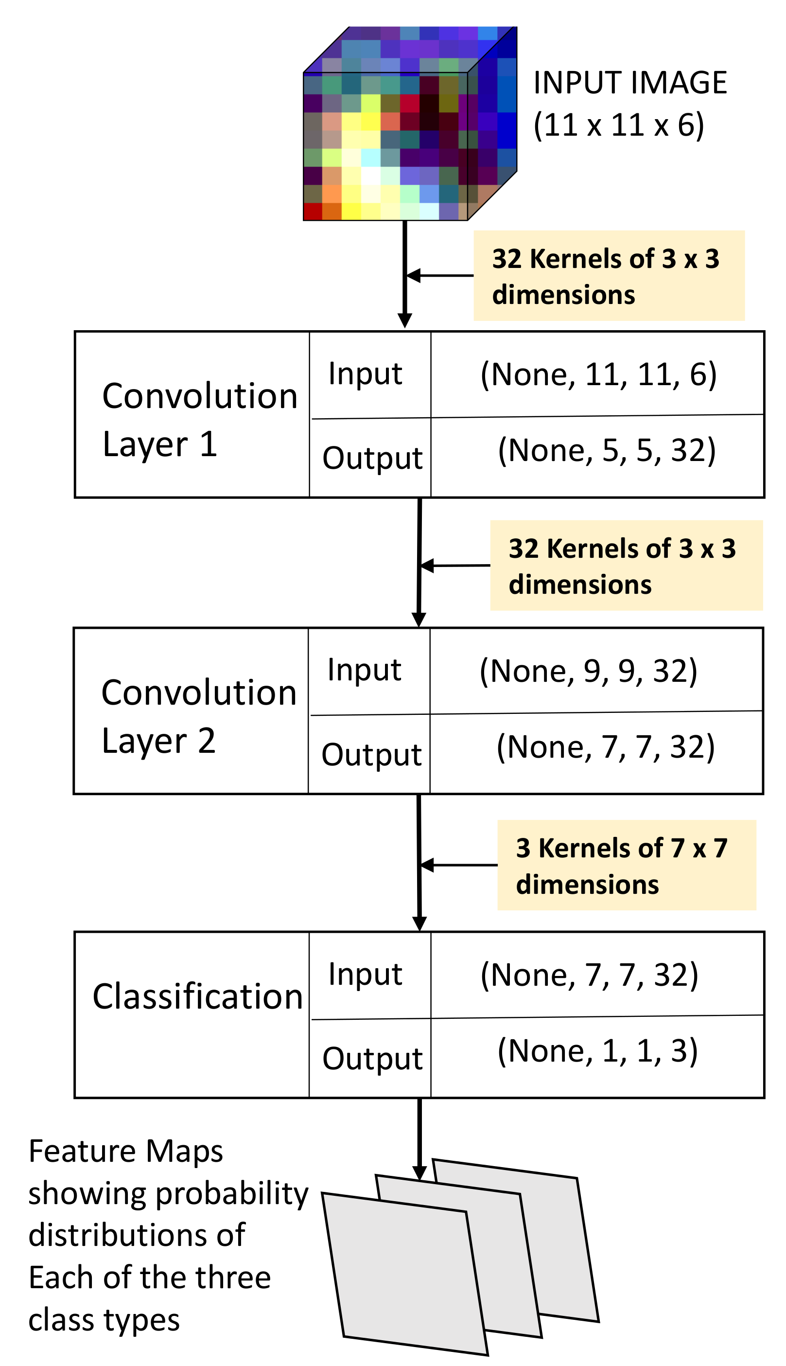
- It is also evident that adding more filters to to the model with 32 learnable filters does not have any effect on model’s test performance proving that the model achieves its optimum level of performance. Therefore, we have finally selected 32 learnable filters as best choice for L1 and L2 convolutional layers and N-3 as best size of neighbourhood window for this study.
3.2. Evaluation of Classification Performance of the F-CNNs Model on Test Images
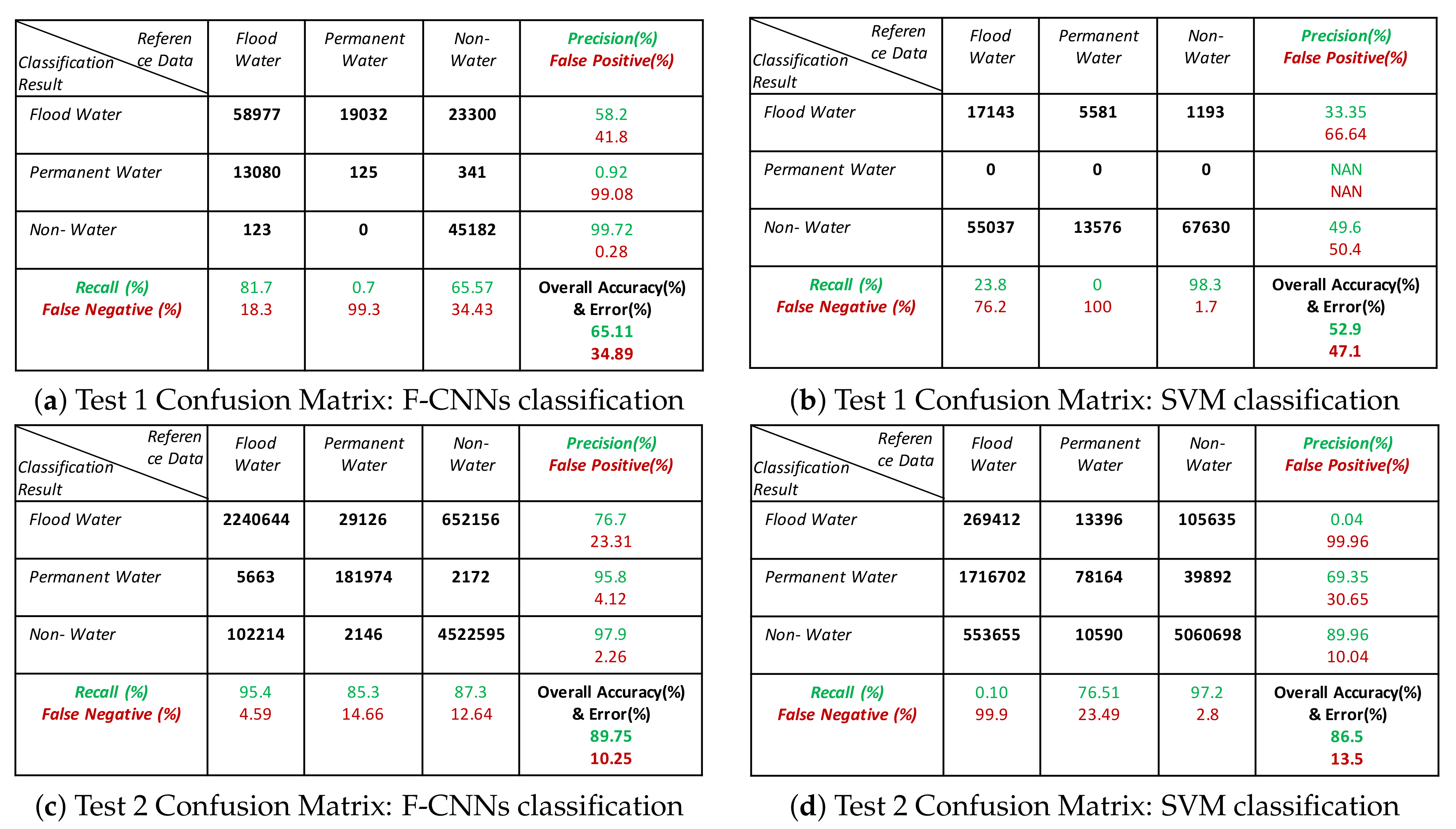
- The classification results show that our proposed model is able to detect flood pixels compared to SVM classifier. The accuracy measures in Figure 10a for Test-1 shows that the recall rate of flood water class is 81.7% which means that the classification model able to detect 81.7% flooded pixels accurately. Compared to F-CNNs, the conventional SVM classification only detects 23.8% (Figure 10b) flood pixels accurately. Much of the flooded pixels are classified as land or non-water by SVM classifier which lowers down the precision rate of non-water class to 49.6%.
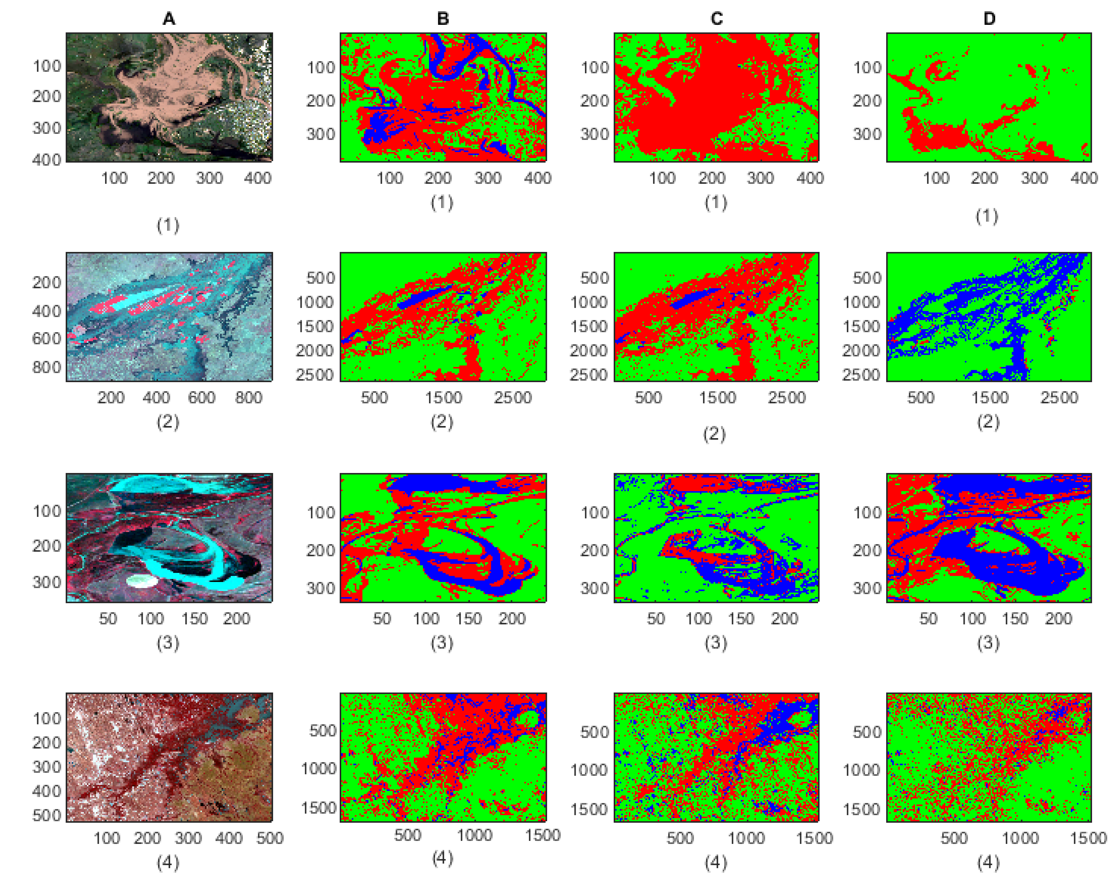
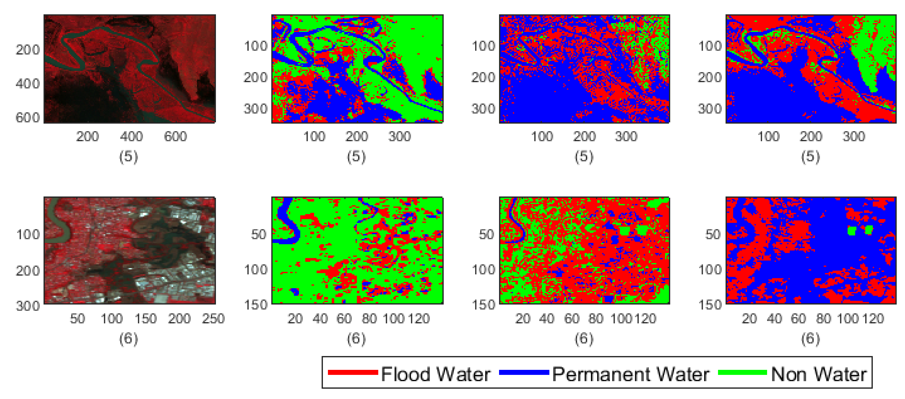
- Both the classification model fails to detect the permanent water from Test-1 image. While F-CNNs model detect permanent-water pixels as flood water (Figure 9(C-1)), SVM classifier misclassifies a considerable amount of flood water pixels and permanent water pixels (Figure 9(D-1)) as non-water class.
- The classification results (Figure 9(C-2,D-2)) of Test image-2 (Figure 9(A-2)) show that the F-CNNs model distinguishes between flood water and permanent water areas with 95.4% recall rate for flooded area detection (Figure 10c) while SVM classifier classifies the entire flooded areas as permanent water features and achieved as low as 0.10% recall rate (Figure 10d).
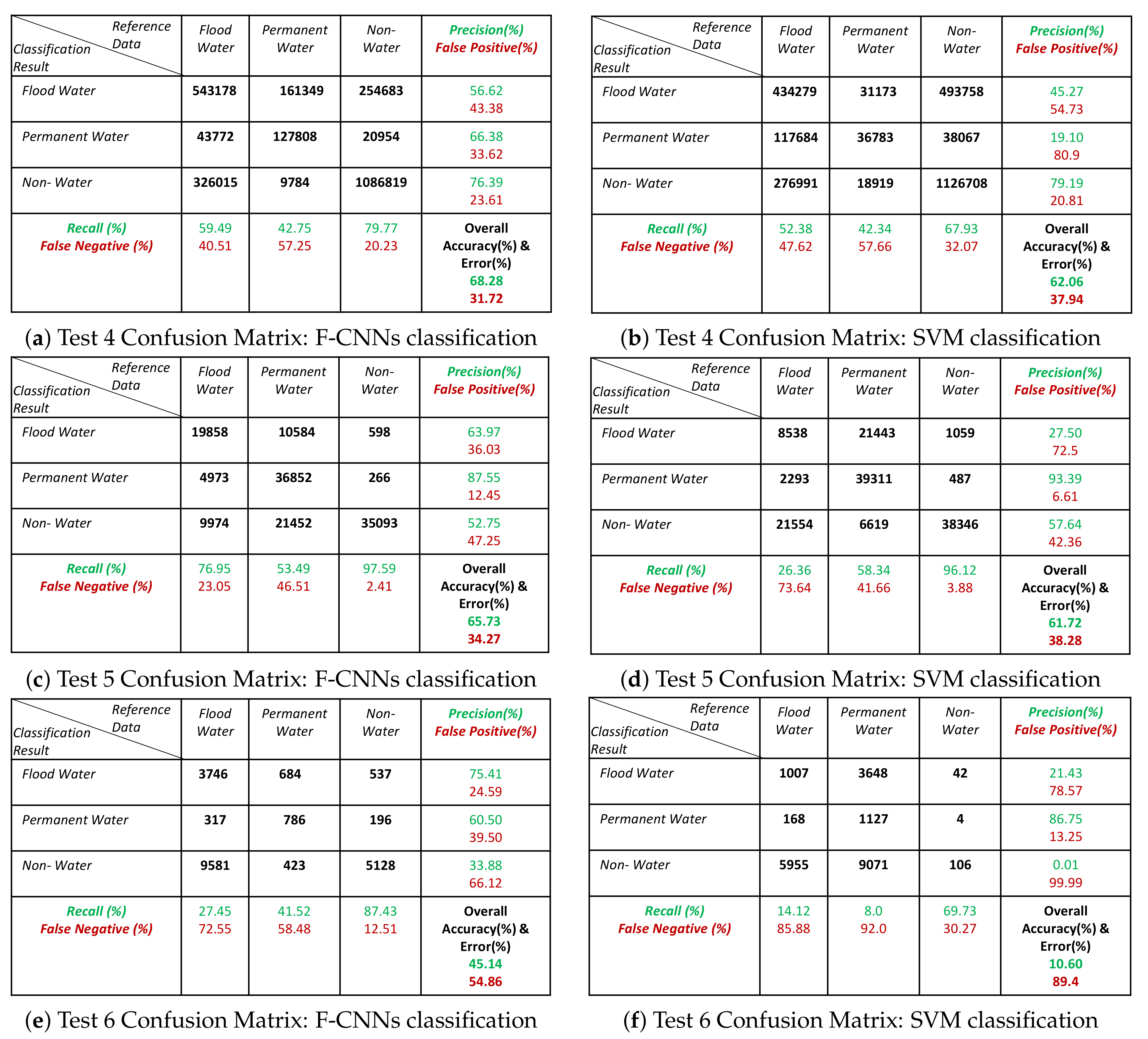
- Both the classification methods on Test-5 achieved with an overall accuracy less than 50%. However, the overall accuracies obtained by F-CNNs model ( 45.14%) is higher than the overall accuracy obtained by SVM classifiers (10.60%).
- However, the F-CNNs model does not able to achieve more than 70% overall accuracy level for every classification tasks, but it is clear from the results that the model is able to distinguish flood water from permanent-water features that the SVM classification method is not able to obtain as we observed in Figure 9(D-2) and Figure 9(D-6).
- Accuracy level of non-water area detection from all test images for both the classification method are showing more than 50% accurately classified pixels except for Test-6 where the SVM classification results show (Figure 9(D-6) and Figure 11f) all the non-water pixels are misclassified as flood waters.
- The overall classification performance also show that F-CNNs model achieves classification accuracy higher than SVM classifiers except in case of Test- 3 classification performance where overall accuracies of both the classifiers are more or less similar (overall accuracy 57.71% for F-CNNs classifier and 58.34% for SVM classifier).
4. Discussion
5. Conclusions
Author Contributions
Funding
Acknowledgments
Conflicts of Interest
References
- DNRM. Flood-Ready Queensland- Queensland Flood Mapping Program: Flood Mapping Implementation Kit. Available online: https://www.dnrm.qld.gov.au/__data/assets/pdf_file/0009/230778/flood-mapping-kit.pdf (accessed on 5 March 2018).
- Klemas, V. Remote Sensing of Floods and Flood-Prone Areas: An Overview. J. Coaster Res. 2015, 31, 1005–1013. [Google Scholar] [CrossRef]
- Zazo, S.; Rodríguez-Gonzálvez, P.; Molina, J.L.; González-Aguilera, D.; Agudelo-Ruiz, C.A.; Hernández-López, D. Flood hazard assessment supported by reduced cost aerial precision photogrammetry. Remote Sens. 2018, 10, 1566. [Google Scholar] [CrossRef]
- Liu, X.; Sahli, H.; Meng, Y.; Huang, Q.; Lin, L. Flood inundation mapping from optical satellite images using spatiotemporal context learning and modest AdaBoost. Remote Sens. 2017, 9, 617. [Google Scholar] [CrossRef]
- Ortega-Terol, D.; Moreno, M.; Hernández-López, D.; Rodríguez-Gonzálvez, P. Survey and classification of large woody debris (LWD) in streams using generated low-cost geomatic products. Remote Sens. 2014, 6, 11770–11790. [Google Scholar] [CrossRef]
- Rahman, M.R.; Thakur, P. Detecting, mapping and analysing of flood water propagation using synthetic aperture radar (SAR) satellite data and GIS: A case study from the Kendrapara District of Orissa State of India. Egyptial J. Remote. Sens. Space Sci. 2018, 21, S37–S41. [Google Scholar] [CrossRef]
- Feng, Q.; Gong, J.; Liu, J.; Li, Y. Flood mapping based on multiple endmember spectral mixture analysis and random forest classifier- the case of Yuyao, China. Remote Sens. 2015, 7, 12539–12562. [Google Scholar] [CrossRef]
- Faghih, M.; Mirzaei, M.; Adamowski, J.; Lee, J.; El-Shafie, A. Uncertainty estimation in flood inundation mapping: An application of non-parametric bootstrapping. River Res. Appl. 2017, 33, 611–619. [Google Scholar] [CrossRef]
- Zhao, J.; Zhong, Y.; Shu, H.; Zhang, L. High-resolution image classification integrating spectral-spatial- location cues by conditional random fields. IEEE Trans. Image Process. 2016, 25, 4033–4045. [Google Scholar] [CrossRef]
- Isikdogan, F.; Bovik, A.; Passalacqua, P. Surface water mapping by deep learning. IEEE J. Sel. Topics Appl. Earth Obs. Remote. Sens. 2017, 10, 4909–4918. [Google Scholar] [CrossRef]
- Ogashawara, I.; Curtarelli, M.; Ferreira, C. The use of optical remote sensing for mapping flooded areas. J. Eng. Res. Appl. 2013, 3, 1956–1960. [Google Scholar]
- Du, Y.; Zhang, Y.; Ling, F.; Wang, Q.; Li, W.; Li, X. Water bodies’ mapping from Sentinal-2 imagery with modified normalized difference water index at 10-m spatial resolution produced by sharpening the SWIR band. Remote Sens. 2016, 8, 354. [Google Scholar] [CrossRef]
- Amarnath, G. An algorithm for rapid flood uinundation mapping from optical data using a reflectance differencing technique. J. Flood Risk Manag. 2014, 7, 239–250. [Google Scholar] [CrossRef]
- Huang, C.; Chen, Y.; Wu, J. Mapping spatio-temporal flood inundation dynamics at large river basin scale using time-series flow data and MODIS imagery. Int. J. Appl. Earth Onservation Geoinform. 2014, 26, 350–362. [Google Scholar] [CrossRef]
- Haq, M.; Akhtar, M.; Muhammad, S.; Paras, S.; Rahmatullah, J. Techniques of remote sensing and gis for flood monitoring and damage assessment: A case study of Sindh province, Pakistan. Egypt. J. Remote Sens. Space Sci. 2012, 15, 135–141. [Google Scholar] [CrossRef]
- Villa, P.; Gianinetto, M. Monsoon flooding response: A multi-scale approach to water-extent change detection. In Proceedings of the ISPRS Commission VII Mid-term Symposium Remote Sensing: From Pixels to Processes, Enschede, The Netherlands, 8–11 May 2006; pp. 1–6. [Google Scholar]
- Chignell, S.; Anderson, R.; Evangelista, P.; Laituri, M.; Merritt, D. Multi-temporal independent component analysis and Landsat 8 for delineating maximum extent of the 2013 Colorado Front Range flood. Remote Sens. 2015, 7, 9822–9843. [Google Scholar] [CrossRef]
- Pierdicca, N.; Pulvirenti, L.; Chini, M.; Guerriero, L.; Candela, L. Observing floods from space: Experience gained from cosmo-skymed observations. Acta Astronaut 2013, 84, 122–133. [Google Scholar] [CrossRef]
- Nandi, I.; Srivastava, P.; Shah, K. Floodplain mapping through support vector machine and optical/infrared images from Landsat 8 OLI/TIRS sensors: Case study from Varanasi. Water Resour. Manag. 2017, 31, 1157–1171. [Google Scholar] [CrossRef]
- Kia, M.B.; Pirasteh, S.; Pradhan, B.; Mahmud, A.; Sulaiman, W.; Moradi, A. A artificial neural network model for flood simulation using GIS: Johor River Basin, Malaysia. Environ. Earth Sci. 2012, 67, 251–264. [Google Scholar] [CrossRef]
- Malinowski, R.; Groom, G.; Schwanghart, W.; Heckrath, G. Detection and delineation of localized flooding from WorldView-2 Multispectral Data. Remote Sens. 2015, 7, 14853–14875. [Google Scholar] [CrossRef]
- Richards, J.; Jia, X. Remote Sensing Digital Image Analysis: An Introduction; Springer: Berlin/Heidelberg, Germany, 2006. [Google Scholar]
- Bangira, T.; Alfieri, S.; Menenti, M.; Van Niekerk, A.; Vekerdy, Z. A spectral unmixing method with ensemble estimation of endmembers: Application to flood mapping in the Caprivi floodplain. Remote Sens. 2017, 9, 1013. [Google Scholar] [CrossRef]
- Gomez-Palacios, D.; Torres, M.; Reinoso, E. Flood mapping through principal component analysis of multitemporal satellite imagery considering the alteration of water spectral properties due to turbidity conditions. Geomat. Nat. Hazards Risk 2017, 8, 607–623. [Google Scholar] [CrossRef]
- Bui, D.; Hoang, N.D. A Bayesian framework based on a Gaussian mixture model and radial-basis-function Fisher discriminant analysis (BayGmmKda VI.1) for spatial prediction of floods. Geosci. Model Dev. 2017, 10, 3391–3409. [Google Scholar]
- Dey, C.; Jia, X.; Fraser, D.; Wang, L. Mixed pixel analysis for flood mapping using extended support vector machine. In 2009 Digital Image Computing: Techniques and Applications; IEEE: Melbourne, Australia, 2009; pp. 291–295. [Google Scholar]
- Wang, L.; Jia, X. Integration of soft and hard classifications using extended support vector machines. IEEE Geosci. Remote Sens. Lett. 2009, 6, 543–547. [Google Scholar] [CrossRef]
- Sarker, C.; Mejias, L.; Woodley, A. Integrating recursive Bayesian estimation with support vector machine to map probability of flooding from multispectral Landsat data. In Proceedings of the 2016 International Conference on Digital Image Computing: Techniques and Applications (DICTA), Gold Coast, Australia, 30 November–2 December 2016; pp. 1–8. [Google Scholar]
- Dao, P.; Liou, Y. Object-oriented approach of Landsat Imagery for flood mapping. Int. J. Comput. Appl. 2015, 7, 5077–5097. [Google Scholar]
- Pulvirenti, L.; Chini, M.; Pierdicca, N.; Guerriero, L.; Ferrazzoli, P. Flood monitoring using multi-temporal COSMO-SkyMed data: Image segmentation and signature interpretation. Remote Sens. Environ. 2011, 115, 990–1002. [Google Scholar] [CrossRef]
- Huang, C.; Townshend, J.; Liang, S.; Kalluri, S.; DeFries, R. Impact of sensor’s point spread function on land cover characterization: Assessment and deconvolution. Remote Sens. Environ. 2002, 80, 203–212. [Google Scholar] [CrossRef]
- Gurney, C.M. The use of contextual information in the classification of remotely sensed data. Photogramm. Eng. Remote Sens. 1983, 49, 55–64. [Google Scholar]
- Moggiori, E.; Tarabalka, Y.; Charpiat, G.; Alliez, P. Convolutional neural networks for large-scale remote sensing image classification. IEEE Trans. Geosci. Remote Sens. 2017, 55, 645–657. [Google Scholar] [CrossRef]
- Amit, S.; Aoki, Y. Disaster detection from aerial imagery with convolutional neural network. In Proceedings of the International Electronics Symposium on Knowledge Creation and Intelligent Computing, (IES-KCIC), Surabaya, Indonesia, 26–27 September 2017; pp. 1–7. [Google Scholar]
- Nogueira, K.; Fadel, S.G.; Dourado, Í.C.; Werneck, R.d.O.; Muñoz, J.A.V.; Penatti, O.A.B.; Calumby, R.T.; Li, L.T.; dos Santos, J.A.; Torres, R.d.S. Exploiting convNet diversity for flooding identification. IEEE Geosci. Remote Sens. Lett. 2018, 15, 1446–1450. [Google Scholar] [CrossRef]
- Gebrehiwot, A.; Hashemi-Beni, L.; Thompson, G.; Kordjamshidi, P.; Langan, T. Deep convolution neural network for flood extent mapping using unmanned aerial vehicles data. Sensors 2019, 19, 1486. [Google Scholar] [CrossRef]
- Mueller, N.; Lewis, A.; Roberts, D.; Ring, S.; Melrose, R.; Sixsmith, J.; Lymburner, L.; McIntyre, A.; Tan, P.; Curnow, S.; et al. Water observations from space: Mapping surface water from 25 years of Landsat imagery across Australia. Remote Sens. Environ. 2016, 174, 341–352. [Google Scholar] [CrossRef]
- Timms, P. Warmer Ocean Temperatures Worsened Queensland’s Deadly 2011 Floods: Study. 2015. Available online: https://www.abc.net.au/news/2015-12-01/warmer-ocean-temperatures-worsened-queenslands-2011-flood-study/6989846 (accessed on 18 March 2017).
- Croke, J. Extreme Flooding Could Return in South-East Queensland. 2017. Available online: https://www.uq.edu.au/news/article/2017/01/extreme-flooding-could-return-south-east-queensland (accessed on 18 March 2017).
- Coates, L. Moving Grantham? Relocating Flood-Prone Towns Is Nothing New. 2012. Available online: https://theconversation.com/moving-grantham-relocating-flood-prone-towns-is-nothing-new-4878 (accessed on 18 March 2017).
- Roebuck, A. Queensland Floodplain Management Plan Sets New National Benchmark. 2019. Available online: http://statements.qld.gov.au/Statement/2019/4/9/queensland-floodplain-management-plan-sets-new-national-benchmark (accessed on 29 September 2017).
- Mathworks. Control Point Registration. Available online: https://au.mathworks.com/help/images/control-point626registration.htm (accessed on 13 June 2019).
- Shalabi, A.L.; Shaaban, Z.; Kasasbeh, B. Data Mining: A preprocessing Engine. J. Comput. Sci. 2005, 2, 735–739. [Google Scholar] [CrossRef]
- Rosebroke, D. Understanding convolutions. In Deep Learning for Computer Vision with Python:Starter Bundle, 2nd ed.; PyImageSearch.com: USA, 2018; Available online: https://www.pyimagesearch.com/deep-learning-computer-vision-python-book (accessed on 16 July 2019).
- Kim, P. Convolutional neural network. In Matlab Deep Learning: With Machine Learning, Neural 616 Networks and Artificial Intelligence; Apress: New York, NY, USA, 2017; Chapter 6. [Google Scholar]
- Andrej, K. CS231n: Convolutional Neural Networks for Visual Recognition. 2016. Available online: http://cs231n.github.io/convolutional-networks/ (accessed on 20 August 2019).
- Simonyan, K.; Zisserman, A. Very deep convolutional networks for large-scale image recognition. In Proceedings of the International Conference on Learning Representations, San Diego, CA, USA, 7–9 May 2015. [Google Scholar]
- Liu, S.; McGree, J.; Ge, Z.; Xie, Y. 4- Computer Vision in Big Data Applications; Academic Press: San Diego, CA, USA, 2016. [Google Scholar]
- Kingma, D.; Lei Ba, J. ADAM: A method for stochastic optimization. In Proceedings of the 3rd International Conference for Learning Representations, San Diego, CA, USA, 7–9 May 2015. [Google Scholar]
- Vapnik, V. The Nature oif Statistical Learning Theory; Springer: New York, NY, USA, 1995. [Google Scholar]
- Notti, D.; Giordan, D.; Caló, F.; Pepe, A.; Zucca, F.; Pedro Galve, J. Potential and Limitations of Open Satellite Data for Flood Mapping. Remote Sens. 2018, 10, 1673. [Google Scholar] [CrossRef]
- Lillesand, T.; Kiefer, R.; Chipman, J. Energy interactions with earth surface features. In Remote Sensing and Image Interpretation; John Wiley and Sons, Inc.: Hoboken, NJ, USA, 2008. [Google Scholar]
- Jensen, J. Remote sensing-derived thematic map accuracy assessment. In Introductory Digital Image Processing: A Remote Sensing Perspective, 4th ed.; Pearson Education, Inc.: Glenview, IL, USA, 2004; pp. 570–571. [Google Scholar]
- Keys, C. Towards Better Practice: The Evolution Of Flood Management in New South Wales; Technical Report; New South Wales State Emergency Services: New South Wales, Australia, 1999. [Google Scholar]
- BMT WBM Pty Ltd. Guide for Flood Studies and Mapping in Queensland; Technical Report; Department of Natural Resources and Mines: Queensland, Australia, 2017. [Google Scholar]


| Specification | Description |
|---|---|
| Revisit Time | 16 Days |
| Spatial Resolutions | 30 m (Reflective bands) 120 m (thermal band) |
| Spectral Channels/Bands | Reflective bands: 1. Visible Blue (0.45–0.52 m); 2. Visible Green (0.52–0.60 m); 3. Visible Red (0.63–0.69 m); 4. Near Infrared (0.76–0.90 m); 5. Short wave Infrared (1.55–1.75 m); 7. Mid Infrared (2.08–2.35 m) Thermal band: 6. Thermal (10.40–12.50 m) |
| Scene Size (Size of an image) | 170 km × 185 km |
| Sensors | Thematic Mapper |
| Filter No. | N-1 Test Accuracy | N-3 Test Accuracy | N-5 Test Accuracy | N-7 Test Accuracy |
|---|---|---|---|---|
| 2 | 0.61 | 0.33 | 0.86 | 0.86 |
| 4 | 0.80 | 0.88 | 0.87 | 0.88 |
| 8 | 0.74 | 0.91 | 0.89 | 0.89 |
| 16 | 0.73 | 0.91 | 0.90 | 0.90 |
| 32 | 0.76 | 0.92 | 0.90 | 0.90 |
| 64 | 0.77 | 0.92 | 0.89 | 0.90 |
| 128 | 0.78 | 0.92 | 0.89 | 0.90 |
| 256 | 0.78 | 0.92 | 0.85 | 0.90 |
| Filter No. | N-1 Test Loss | N-3 Test Loss | N-5 Test Loss | N-7 Test Loss |
|---|---|---|---|---|
| 2 | 0.89 | 1.09 | 0.41 | 0.43 |
| 4 | 0.70 | 0.32 | 0.35 | 0.33 |
| 8 | 0.73 | 0.24 | 0.29 | 0.28 |
| 16 | 0.67 | 0.21 | 0.26 | 0.24 |
| 32 | 0.6 | 0.19 | 0.28 | 0.24 |
| 64 | 0.57 | 0.19 | 0.55 | 0.24 |
| 128 | 0.54 | 0.19 | 0.78 | 0.24 |
| 256 | 0.53 | 0.19 | 0.41 | 0.25 |
| Image No. | Name of the Sensor | Date (year/month/day) | Path-Row | Location |
|---|---|---|---|---|
| 1 | Landsat-8 Operational Land Imager (OLI) | 2017/04/04 | 91-76 | Rockhampton, Queensland, Australia |
| 2 | Landsat-5 Thematic Mapper (TM) | 2011/01/21 | 92-80 | Dirranbandi, Queensland, Australia |
| 3 | Landsat-5 Thematic Mapper (TM) | 2011/03/26 | 92-79 | Balonne River, Queensland, Australia |
| 4 | Landsat-5 Thematic Mapper (TM) | 2011/03/28 | 99-79 | Yelpawaralinna Waterhole, Queensland, Australia |
| 5 | Landsat-5 Thematic Mapper (TM) | 2008/03/04 | 106-69 | Daly River Basin, Darwin, Australia |
| 6 | Landsat-5 Thematic Mapper (TM) | 2011/01/16 | 89-79 | Brisbane River, Queensland Australia |
© 2019 by the authors. Licensee MDPI, Basel, Switzerland. This article is an open access article distributed under the terms and conditions of the Creative Commons Attribution (CC BY) license (http://creativecommons.org/licenses/by/4.0/).
Share and Cite
Sarker, C.; Mejias, L.; Maire, F.; Woodley, A. Flood Mapping with Convolutional Neural Networks Using Spatio-Contextual Pixel Information. Remote Sens. 2019, 11, 2331. https://doi.org/10.3390/rs11192331
Sarker C, Mejias L, Maire F, Woodley A. Flood Mapping with Convolutional Neural Networks Using Spatio-Contextual Pixel Information. Remote Sensing. 2019; 11(19):2331. https://doi.org/10.3390/rs11192331
Chicago/Turabian StyleSarker, Chandrama, Luis Mejias, Frederic Maire, and Alan Woodley. 2019. "Flood Mapping with Convolutional Neural Networks Using Spatio-Contextual Pixel Information" Remote Sensing 11, no. 19: 2331. https://doi.org/10.3390/rs11192331
APA StyleSarker, C., Mejias, L., Maire, F., & Woodley, A. (2019). Flood Mapping with Convolutional Neural Networks Using Spatio-Contextual Pixel Information. Remote Sensing, 11(19), 2331. https://doi.org/10.3390/rs11192331


