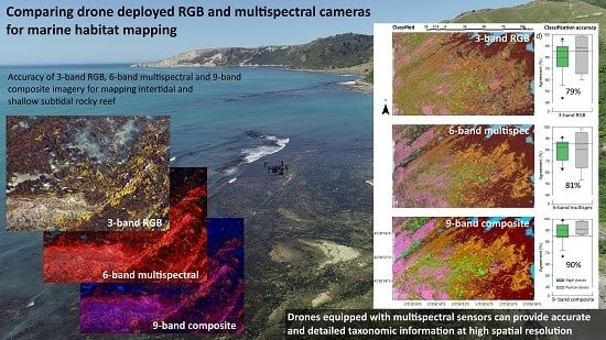
Unmanned Aerial Vehicles (UAVs) for Monitoring Macroalgal Biodiversity: Comparison of RGB and Multispectral Imaging Sensors for Biodiversity Assessments

Abstract

Developments in the capabilities and affordability of unmanned aerial vehicles (UAVs) have led to an explosion in their use for a range of ecological and agricultural remote sensing applications. However, the ubiquity of visible light cameras aboard readily available UAVs may be limiting the application of these devices for fine-scale, high taxonomic resolution monitoring. Here we compare the use of RGB and multispectral cameras deployed aboard UAVs for assessing intertidal and shallow subtidal marine macroalgae to a high taxonomic resolution. Our results show that the diverse spectral profiles of marine macroalgae naturally lend themselves to remote sensing and habitat classification. Furthermore, we show that biodiversity assessments, particularly in shallow subtidal habitats, are enhanced using six-band discrete wavelength multispectral sensors (81% accuracy, Cohen’s Kappa) compared to three-band broad channel RGB sensors (79% accuracy, Cohen’s Kappa) for 10 habitat classes. Combining broad band RGB signals and narrow band multispectral sensing further improved the accuracy of classification with a combined accuracy of 90% (Cohen’s Kappa). Despite notable improvements in accuracy with multispectral imaging, RGB sensors were highly capable of broad habitat classification and rivaled multispectral sensors for classifying intertidal habitats. High spatial scale monitoring of turbid exposed rocky reefs presents a unique set of challenges, but the limitations of more traditional methods can be overcome by targeting ideal conditions with UAVs.

1. Introduction

Kelp and macroalgal ecosystems cover a large proportion of the earth’s coastlines [1], support diverse and productive ecosystems [2], and are some of the most prolific carbon fixers on the planet [3]. These habitats on rocky shores are a key component of temperate marine ecosystems, providing a variety of ecosystem services, producing biomass for consumers within and far outside of kelp beds, and contributing to carbon sequestration in deep sediments [4]. Kelp distributions are declining globally [3], with warming trends and heatwave events causing the dramatic contraction of kelp beds in some regions [5,6,7]. Understanding the consequences of global climate change and other spatially explicit stressors (e.g., eutrophication, sedimentation) requires broad-scale assessments of spatial distributions and biodiversity.

Although imaging sensors aboard satellites have been frequently used for mapping terrestrial vegetation [8,9,10] and specific marine vegetation (e.g., Macrocystis pyrifera, [11,12,13]; Nereocystis leutkeana, [14]; and seagrass [15,16]), there are several limitations to using satellite imagery to assess multiple habitat classes simultaneously, particularly in patchy habitats [17]. Marine assemblages often form highly variable mosaics associated with a range of environmental and biological gradients [18,19]. In such cases, pixel resolution can be problematic for habitat classification, where spectral signatures of multiple vegetation types are dampened (spectral confusion) [17]. Furthermore, satellite imagery is greatly affected by meteorological conditions, such as cloud and aerosol interference, surface glare, and poor synchrony with tides. For many applications these limitations are absorbed by the high frequency of satellite passes. However, the chances of capturing high-quality images diminish greatly in turbid coastal waters where accurate observations of the intertidal and subtidal zones require aligning tide, meteorological, and oceanographic variables. Autonomous unmanned aerial vehicles (UAVs, commonly referred to as “drones”) deployed to coincide with meteorological and oceanographic conditions provide a potential alternative, allowing the targeting of key meteorological variables and performing moderate-scale mapping of intertidal and shallow subtidal kelp and macroalgae beds [20].

UAVs are increasingly being used for a range of environmental and ecological monitoring campaigns [20,21,22,23,24,25,26,27] and, although the use of aerial platforms for ecological monitoring is hardly new, the deployment of imaging sensors on unmanned aerial drones has some advantages (as well as disadvantages) over other manned and unmanned platforms. The key advantages of copter drones are high pixel resolution, highly flexible deployment, and relatively low cost per unit of time [25,28]. Satellite platforms provide the cheapest option, especially per unit area, but suffer from low pixel resolution and are restricted in the timing of imagery capture. One key benefit of satellite imagery is the multiple discrete spectral bands available, particularly infrared bands that allow enhanced vegetation detection [29]. However, the adaptation of multi-spectral and hyper-spectral imaging systems to drone platforms in some ways closes the gap between low spatial resolution, high spatial coverage satellite imagery, and traditional ecological monitoring techniques with high taxonomic resolution and accuracy, but very low spatial coverage [25].

The dissipation of infrared wavelengths during the active photosynthesis of vegetation provides a reflection of electromagnetic radiation in specific wavelengths (710–800 nm) and has been well used in terrestrial applications for the remote sensing of vegetation, including biomass estimation and assessments of vegetation health [8,9,10]. However, the rise of aerial drones for ecological research has been dominated by units equipped with visible light cameras (known as RGB because of the three bands of data representing the intensities of red, green, and blue wavelengths of each pixel [20,23]). Additional spectral bands (i.e., not only red-green-blue) provide further opportunities to identify unique spectral signatures among vegetation types. In this sense, marine macroalgae provide great opportunities for high species separation compared to terrestrial plants, because of their high photosynthetic pigment diversity [30,31,32]. Marine macroalgae fall across three phyla—Ochrophyta (brown algae), Chlorophyta (green algae), and Rhodophyta (red algae)—with each showing unique pigment profiles [33], and species within each phylum showing high variability in some cases [30,32]. The spectral separation of the return reflection signal potentially provides utility in more detailed broad-scale mapping of macroalgal communities with high species richness. The detection of these unique spectral profiles may be enhanced by isolating key parts of the electromagnetic spectrum using multispectral imaging with discrete, non-overlapping bands.

Here we examine the effectiveness and accuracy of UAVs for separating diverse species mixtures of intertidal and shallow subtidal macroalgae. Autonomous UAVs are readily and cheaply available to a range of specialist and citizen scientists and are commonly purchased with RGB (red-green-blue) cameras. Vegetation detection is notably improved by measuring reflection in the near-infrared wavelengths [34], but infrared wavelengths are heavily absorbed by water, making them less useful with increasing water depth. We examined the relative benefits of enhanced spectral sensing over more readily available RGB sensors to (a) determine the potential applications and limitations of readily available sensors, and (b) determine the potential of enhanced spectral sensors for marine macroalgal taxonomic separation across intertidal and shallow subtidal habitats in turbid and exposed environments.

2. Materials and Methods

2.1. Study Site

The Oaro reef is a limestone platform in the Kaikoura region of the South Island of New Zealand (Figure 1). This is an open coast rocky reef exposed to oceanic swell but with several fringing rocky platforms that can buffer all but the largest swells. These rocky intertidal and subtidal platforms have one of the richest macroalgal floras in New Zealand, with over 200 individual species of Ochrophyta (brown algae), Rhodophyta (red algae), and Chlorophyta (green algae) identified [35]. Several long-term studies have examined small-scale, high-resolution biodiversity [35,36], making it an ideal location to upscale macroalgal biodiversity assessments using UAVs. Much of this biodiversity is unlikely to be identifiable from above due to the spatial and temporal rarity of many species [35] and the occurrence of many species beneath canopies [37]. However, several canopy-forming brown algal species (Hormosira banksii, Carpophyllum maschalocarpum, Durvillaea spp.) occur at high abundance at this site, and there are also large stands of red (Gigartina spp., Cladhymenia oblongifolia, Corallina officinalis) and green (Ulva spp.) macroalgal species. The high algal richness and broad taxonomic variation make this an ideal location to examine the potential for UAVs to perform broad-scale biodiversity assessments of major habitat-dominating algae.

2.2. Macroalgal Richness and Spectral Profiles

The species richness of algae across the study site was assessed at two tidal zones (mid and low shore). At each shore height, the cover and identity of macroalgal species were enumerated and identified using permanent transects and 1 m² quadrats. A subset of these species from each phylum—Ochrophyta (brown algae), Rhodophyta (red algae), and Chlorophyta (green algae)—was selected for determining spectral signals.

The spectral signature of macroalgal reflection was determined for a number of key macroalgal species in the region. An Ocean Optics^® spectrometer (350–1000 nm range, band width of 0.3 nm) was used to identify the spectra reflected by macroalgal thalli. Samples were illuminated with a tungsten-halogen light source within an integrating sphere (ISP-REF, OceanOptics^®) for reflectance measurements. Before testing reflection spectra, dark calibration and a white standard (Spectralon 99%) were used for calibration and all data were collected using the OceanView (OceanOptics^®) software. In all cases, four replicate specimens of each species were used, with the combined spectra of the four replicates averaged for each species. Reflection signals of each macroalgal thallus were averaged over 5 nm widths, and all four replicates were then averaged, and the standard error was estimated. Although the remarkably high species richness of this site makes it difficult to examine the spectral signatures of all individual species, we sampled several species across the Phaeophyceae, Rhodophyta, and Chlorophyta. Species representing Ochrophyta (Carpophyllum maschalocarpum, Macrocystis pyrifera, and Hormosira banksii), Rhodophyta (Cladhymenia oblongifolia, Champia novaezealandiae, and Polysiphona sp.) and a single Chlorophyte (Ulva spp.) were assessed for reflection spectra. Reflection spectra were standardized by peak reflection at wavelengths between 700 and 720 nm.

2.3. UAV Mapping

The capture of RGB and multispectral aerial imagery for habitat classification was completed at the Oaro reef in February 2019 over 0.4 km² of rocky reef (Figure 2). A DJI Matrice 600 equipped with both an Airphen^® (Hiphen^®) six-band multispectral camera and a Sony mirrorless RGB camera was used to capture imagery. The Airphen^® multispectral camera has a focal length of 8 mm, a sensor resolution of 1280 × 960 pixels, and six synchronized global shutter sensors each centered at 530, 570, 630, 670, 710, and 750 nm (band width 10 nm). The three bands of the Sony^® RGB camera span the visible wavelengths (400–700 nm), with large overlap between blue and green and green and red, but little overlap between red and blue. The Sony camera was an A5100 with a 15 mm Voitlander^® rectilinear lens, providing final images of 6000 × 4000 pixels. Flights were completed during clear sky conditions, during the lowest tide series of the month (one of the best tide series of the year) and were completed within 30 minutes each side of peak low tide. Marine conditions were also favorable with a swell <0.8 m (significant wave height). Flights were at an elevation of 50 m above sea level and single images were taken with 95% overlap (RGB) and 80% overlap (multispectral camera); image capture on both cameras was triggered simultaneously.

To geo-reference the orthoimages accurately, 12 ground control targets were laid out evenly across the captured area. These targets were 0.5 × 0.5 m with high contrast blue and yellow squares to accurately identify the center of the target. Each target was surveyed using a high accuracy RTK-GPS system (Trimble™). Furthermore, 3 × 30 meter transects were laid out across the reef with weighted bright orange cones positioned at 10 m intervals along each tape. Transects were dominated by intertidal habitat, with only around 15% of transects covering shallow subtidal habitats. The cover and diversity of macroalgae were assessed and photographed in situ in 30 × 0.25 m² quadrats at 1 m intervals along each transect to provide ground truthing of species composition. The positions of the quadrats and relative species assessments were used to produce validated training samples on the whole reef orthoimage.

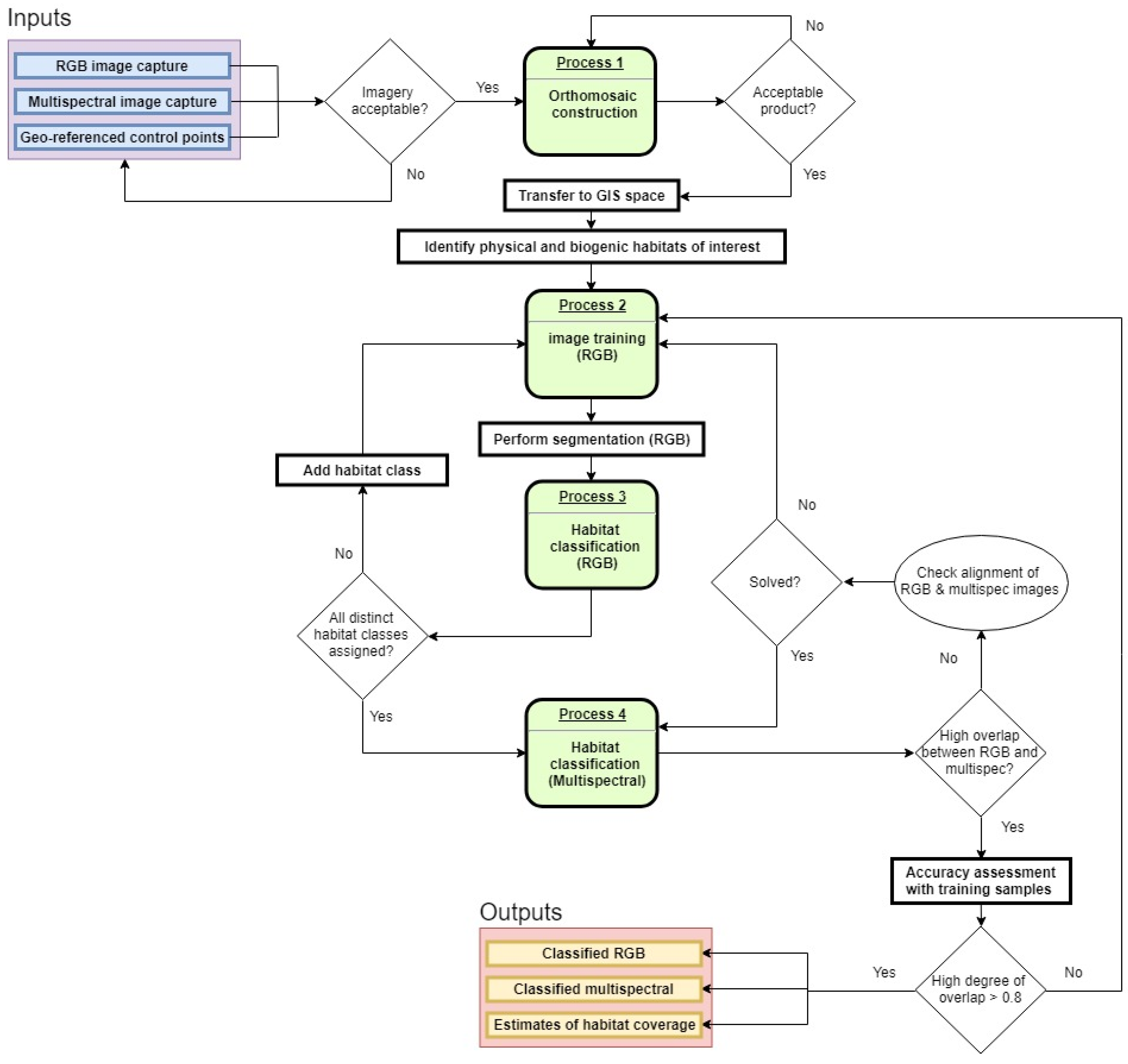
2.4. Analysis and Validation

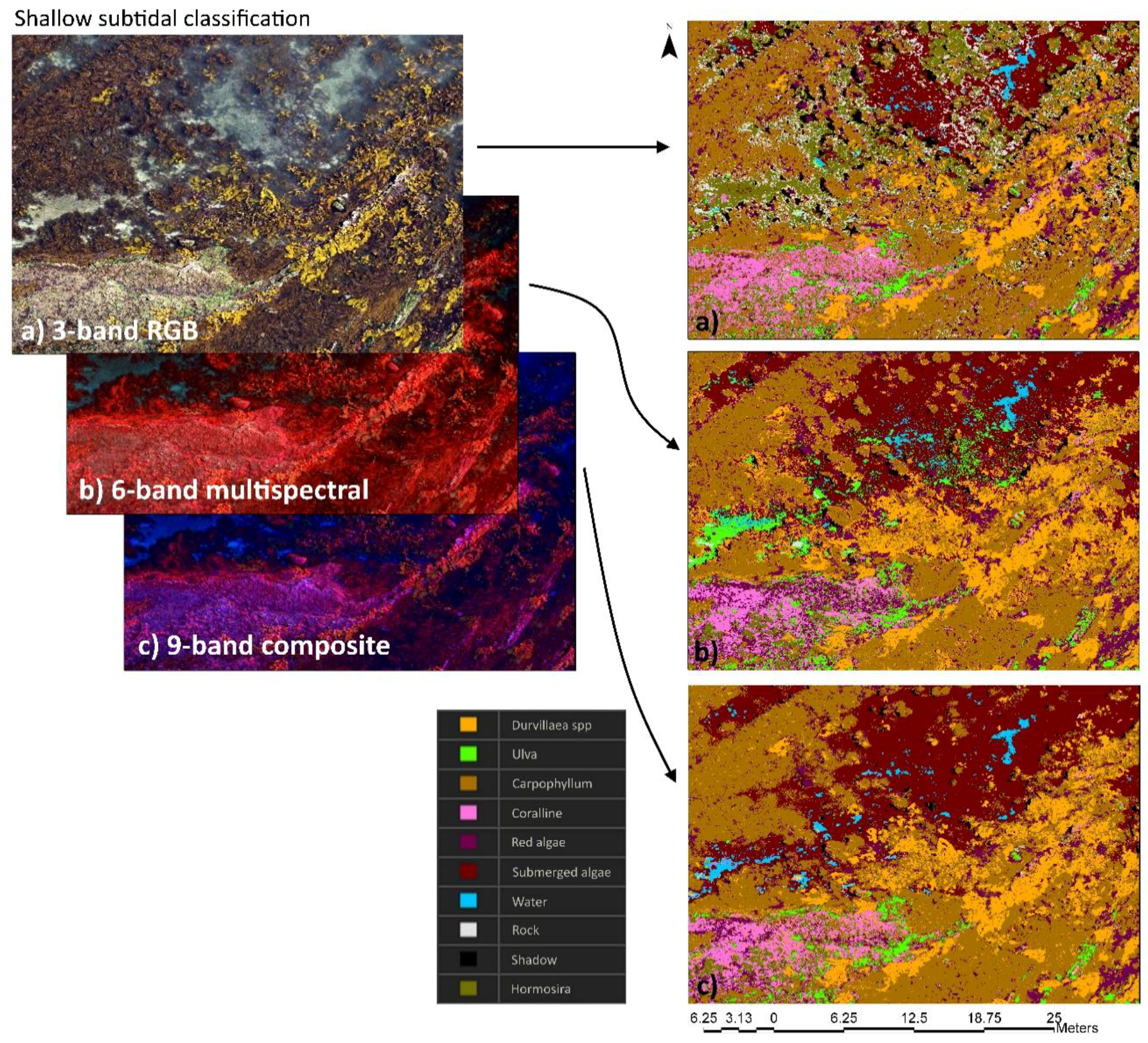
RGB imagery (8 bit) was stitched together using Agisoft Photoscan™. The final orthoproduct was a three-band image with a final pixel size of 1.25 cm² per pixel. Multispectral images (32 bit) were stitched together using Agisoft Photoscan™, as well as the Airphen™ plugin for multiband imagery. The final product was a six-band orthomosaic with 2.5 cm² pixels. Reflectance was calibrated using a reference panel and the radiometric calibration tool (Agisoft Photoscan™ and the Airphen™ plugin). Values from the RGB camera represent brightness alone. Additionally, the RGB and multispectral orthomosaics were combined into a composite nine-band orthomosaic by aligning the ground control targets from each orthomosaic. To do this, the six band multispectral dataset was resampled using bilinear interpolation to produce the same pixel size as the RGB imagery (1.25 cm² pixels). The composite imagery therefore combined the three broad bands of RGB and the six narrow bands of the multispectral camera, as well as combining the finer-scale pixel resolution of the RGB images with the coarser-scale multispectral images.

Habitat classification procedures were done on a per pixel basis using support vector machines (SVM) trained using 50 training samples per class (Arc GIS Pro™). Samples were polygons selected around habitat classes encompassing, in some cases, several hundred pixels. The assigned classes were: Durvillaea spp.; Carpophyllum (mostly Carpophyllum maschalocarpum, also including the occasional Cystophora sp.); Ulva spp.; red algae; Hormosira banksii; coralline algae (including articulated and crustose coralline algae); a generic algal class not readily identifiable to species due to increasing depth (but still identifiable as vegetation); bare rock; water (with no visible submerged vegetation); and shadow. Furthermore, an additional 50 unique samples of each class were retained for validation procedures (hereafter referred to as remote validation samples). On top of these remote validation samples, in situ validation regions along the three delineated transects were also identified for accuracy testing. These samples, unlike the validation samples, had uneven sample sizes of each class, but provided higher resolution at a small scale. Images taken at ground level were GPS-referenced and embedded into the whole region orthoimage, enabling the sampling of validation regions of the habitat classes. Remote and in situ validation samples were assessed using the high-resolution RGB imagery, where the color and shape of each habitat class was readily identifiable. Once samples were generated on the RGB images, the habitat classification was completed separately for RGB imagery, multispectral imagery, and composite imagery (three-band RGB + six-band multispectral). The workflow for these procedures is shown in Figure 3.

For accuracy assessments, confusion matrices were generated and the user accuracy, producer accuracy, Cohen’s kappa, and combined agreement between reference samples and the classified maps were determined. Furthermore, errors of omission (Type I errors) and errors of commission (Type II errors) were also calculated for each class. This was done separately for the remote validation and the in situ validation samples. Accuracy assessments used 10,000 random points and an equalized stratified random sampling strategy which equally distributes random points across each class. Accuracy assessments were done on RGB imagery, multispectral imagery, and the composite image (three-band RGB + six-band multispectral).

3. Results

Full macroalgal biodiversity surveys completed prior to aerial surveys revealed a total of 45 macroalgae, represented by three green algae, 15 brown algae, and 27 red algae (Appendix A). Low shore assemblages had only a single green alga, 10 brown algae, and 26 red algae. Mid-shore assemblages in contrast had more green algae (three species) and higher brown algal richness (12 species), but lower red algal richness (19 species).

The reflection spectra of brown, green, and red macroalgal species showed clear spectral separation between groups (Figure 3). In general, red algae showed reduced reflection between 520 and 650 nm wavelengths compared to brown algae, while green algae showed consistent but low reflection at most wavelengths except blue. The spectral sensitivity of RGB sensors integrate wavelengths that span peak absorption and reflection (e.g., 600–700 nm), but the blue (400–500 nm) band spans wavelengths not covered by the multispectral sensor (Figure 4a). In contrast, the bands of the multispectral camera are at wavelengths corresponding to high absorption (troughs) and high reflection (peaks). Red algal species (Cladhymenia oblongifolia, Champia novaezealandiae, and Polysiphonia sp) had some crossover, but overall showed unique signatures, particularly at near-infrared wavelengths (Figure 4b). The two fucoid species of brown algae (Hormosira banksii and Carpophyllum maschalocarpum) had similar spectral profiles (Figure 4c), but with some separation of the two species at the peak absorption of chlorophyll-a (670 nm). The single laminarian brown alga (Macrocystis pyrifera) varied greatly from the fucoid species. The green algae (Ulva spp.) had lower reflection overall than the red or brown species, with few distinct peaks of reflection or absorption (Figure 4d). The spectral bands captured by the multispectral camera were positioned at suitable wavelengths for separating macroalgal species, particularly between red, brown, and green algae, but may lack the spectral resolution for separating species with similar spectral profiles within phyla.

Imagery revealed that a number of species were readily identifiable from 50 m altitude (Figure 5a–c). However, not all species detected in situ were identifiable from aerial imagery, and so several species were combined into functional groups. Habitat classification of three-band RGB imagery, six-band multispectral imagery, and nine-band composite imagery showed comparable results (Figure 5e), but on closer inspection there were some differences within increasing spectral bands. In particular, nine-band composite imagery had >85% agreement between reference and classified datasets, while three-band RGB and six-band multispectral imagery had <85% agreement for algal classes (Figure 5e). Habitat classification of intertidal regions had relatively high rates of agreement between three-band, six-band, and nine-band imagery, although there was much greater patchiness of the three-band RGB dataset and greater connectedness of classes for the six-band multispectral and nine-band composite datasets (Figure 6). Subtidal regions showed a high rate of misclassification of Carpophyllum in the three-band RGB imagery, which was frequently misclassified as Hormosira, bare rock, and shadow (Figure 7). In fact, one of the common misclassifications of the RGB dataset was the classification of vegetation classes as null classes, particularly bare rock or shadow. Subtidal classification of multispectral imagery also frequently misclassified water (with bare rock beneath) as Ulva. Both misclassification errors were not obvious in the composite imagery. There was also a tendency for shallow submerged vegetation to be grouped into the generic submerged algae class, which included red algal species, coralline algae, and brown kelp and fucoid species.

Over the entire study area, RGB and multispectral imagery frequently misclassified several habitat classes (i.e., 1/5 pixels assigned to a class were misclassified), though these classes differed between the two imagery types. Multispectral imagery frequently misclassified Ulva and Durvillaea spp., whereas bare rock, coralline algae, Hormosira, and Carpophyllum were frequently misclassified by the RGB imagery (

Table 1. Accuracy assessment of habitat classification for three-band RGB, six-band multispectral, and nine-band composite imagery, including the accuracy of each class (user accuracy “U-acc” and producer accuracy “P-acc”), the combined agreement between classified data and reference data (“Agreement %”), and the Cohen’s kappa estimate of accuracy (negative values indicate that classification is significantly worse than random; values close to 1 indicate that classification is significantly better than random). Accuracy was assessed from validation samples collected in two ways: directly from imagery (remote validation) and from ground truth samples from three transects captured in the orthoimages (in situ validation). Bold values highlight the imagery type that had the lowest rate of misclassification.

	Remote Validation						In Situ Validation
	Three-band		Six-band		Nine-band		Three-band		Six-band		Nine-band
Class	U-acc	P-acc	U-acc	P-acc	U-acc	P-acc	U-acc	P-acc	U-acc	P-acc	U-acc	P-acc
Durvillaea spp.	0.88	0.71	0.76	0.71	0.89	0.78	0.72	0.96	0.63	0.91	0.79	0.96
Ulva	0.87	0.92	0.65	0.91	0.94	0.95	0.97	0.92	0.7	0.84	0.93	0.92
Carpophyllum	0.7	0.8	0.85	0.86	0.84	0.89	0.71	0.87	0.86	0.7	0.79	0.92
Coralline	0.71	0.89	0.84	0.81	0.84	0.83	0.72	0.79	0.7	0.84	0.81	0.9
Red algae	0.89	0.79	0.8	0.84	0.82	0.84	0.91	0.44	0.8	0.62	0.88	0.9
Submerged algae	0.82	0.73	0.75	0.65	0.84	0.98	-		-		-
Hormosira	0.55	0.66	0.82	0.91	0.89	0.9	0.62	0.71	0.67	0.76	0.73	0.86
Rock	0.75	0.6	0.98	0.53	0.98	0.87	0.82	0.99	0.98	0.68	0.99	0.99
Shadow	0.92	0.84	0.99	0.99	0.99	0.99	0.88	0.67	0.99	0.74	0.99	0.99
Water	0.99	0.99	0.61	0.94	0.98	0.95	0.99	0.93	0.76	0.83	0.99	0.87
Agreement %	79%		81%		90%		81%		77%		88%
Cohen’s Kappa	0.77		0.79		0.89		0.79		0.75		0.87

). In contrast, composite imagery (combined RGB + multispectral) had low rates of misclassification (better than 1/10 pixels misclassified for most classes). In all cases the highest degree of misclassification was for the fucoid algae, Hormosira banksii and Carpophyllum maschalocarpum, which, according to the reflectance profiles (Figure 4), were the most similar of any two species examined.

In general, the accuracy of remote validation samples was higher than that for in situ validation samples. However, this was not the case for RGB imagery, which had slightly lower rates of misclassification for in situ validation samples (Table 1; Appendix B). This may be associated with the dominance of intertidal habitat in the validation transects and the low sample size of several subtidal habitat classes. Combining three broad bands and six narrow bands of RGB and multispectral cameras provided the best results for the classification of marine macroalgae (ca. 1/10 pixels misclassified, compared to ca. 1/5 pixels misclassified for both RGB and multispectral imagery).

4. Discussion

Marine macroalgae are a key component of coastal ecosystems worldwide, and in many marine temperate systems they are the key habitat-formers and ecosystem engineers. Loss of marine macroalgae is often associated with the collapse of many essential ecosystem functions [38], with metrics of macroalgal richness and abundance therefore representing an integrated assessment of ecosystem health. These habitat-formers are threatened by a spatial hierarchy of anthropogenic disturbances, from local-scale point source discharges of sediments/pollutants [39,40] and regional-scale overfishing [41] to global-scale climate change [6,42]. Although the use of satellite sensors for monitoring some temperate macroalgal species is well established [11,12,13,14], these techniques are not reliable in all situations and do not enable the estimation of the relative cover of several overlapping species.

Targeting optimal meteorological and oceanographic conditions for high-resolution remote sensing with UAVs ideally fills a gap between high spatial cover, low-resolution satellites and low spatial cover, high-resolution in situ sampling [25,27]. High-resolution remote sensing using UAVs has great potential to detect changes in rocky reef ecosystems, but importantly may have the spatial and taxonomic resolution to detect subtle changes preceding ecological collapse (i.e., tipping points). Such subtle cues may include (a) species displacement (e.g., replacement of native Durvillaea spp. by invasive Undaria pinnatifida [7]), (b) distribution shifts at fringes of exposure [43,44], and (c) shifts in species compositions/richness/distributions.

Our results confirm that UAVs are a useful tool for the identification of multiple intertidal habitat types (see also [20,23,24,26]). Multispectral sensors aboard UAVs for high-resolution multiband imagery have, to our knowledge, not been used on temperate coastal marine environments. Spectrally rich imagery has enormous potential for producing spatial distribution maps of macroalgal distribution at relatively high taxonomic resolution. We showed the separation not only of broad taxonomic groupings (Ochrophyta, Rhodophyta, and Chlorophyta), but also of species within phyla. There are, however, limitations to the depth at which sufficiently unique spectral signals are returned, and limitations to the distinctness of spectral profiles that can be separated. For example, two spectrally similar species (the fucoids Hormosira banksii and Carpophyllum maschalocarpum) had the highest rates of misclassification.

UAVs are becoming a ubiquitous tool in local-scale remote sensing research [25,28]. However, the best practices and limitations of these tools for marine coastal biodiversity assessments are yet to be established. Our study highlights the potential of UAVs to accurately assess the richness of marine macroalgal vegetation in intertidal and shallow subtidal environments, but also strongly recommends the use of multispectral imaging systems (or hyperspectral systems) for detecting unique spectral signatures and maximizing taxonomic resolution. Habitat classification accuracy was greater when combining the broad spectral ranges of RGB bands and the narrow multispectral bands, suggesting that greater spectral resolution would lead to increasing accuracy and greater taxonomic resolution. However, RGB (three-band) imagery did perform remarkably well compared to composite (nine-band) imagery in classifying intertidal habitats, suggesting that imagery from readily available drones could be useful in determining broad-scale coverage of multiple intertidal habitat types [20,24,26]. This research promotes the use of RGB cameras aboard UAVs for high spatial resolution studies of intertidal macroalgal coverage but urges caution in the number of habitat classes that can be readily separated and suggests that immersed habitats may have insufficient spectral information to be classified accurately.

Regardless of the spectral resolution of the imaging system, there were limitations in the application of aerial tools for mapping submerged habitats. The dampening of spectral signals with increasing water column depth only allows the detection of taxonomically broad submerged algal classes. Beyond a depth of 2–3 m in turbid coastal waters, the accurate detection of any vegetation classes should be treated with caution. There were also limitations in the use of in situ transects for validating habitat classification procedures at a broad scale. The relatively small scale covered by in situ transects and the patchy nature of macroalgal assemblages can result in an uneven distribution of validation samples across habitat classes. We recommend trialing multi-height UAV flights (e.g., discrete 20 m altitude strips within an area mapped at 50 m altitude) to produce extremely high-resolution imagery over narrow strips (ideally including survey features such as transects and markers) to enable accurate validation sample collection, potentially leading to a greater separation of taxonomic richness.

There is, however, great potential in multispectral and hyperspectral sensing for the high taxonomic separation of intertidal and shallow macroalgal species [45], and potentially enhanced signature detection through increasing distances of water column with increasing band resolution. Multispectral imaging was more accurate than RGB imagery; however, combining the broad RGB signal with the narrow multispectral imagery produced high rates of accurate habitat classification. Hyperspectral imaging has been successfully used to separate even optically similar species, such as multiple species of seagrass [16], and a higher spectral resolution may be necessary for species-level classification in some cases (e.g., separating spectrally similar species such as Hormosira and Carpophyllum). Compact field deployable hyperspectral systems hold much promise for many applications [46], and their use for classifying marine macroalgae could allow species-level identification over moderate spatial scales.

5. Conclusions

Exposed coastal rocky reef ecosystems are particularly challenging habitats to monitor for several reasons: (a) they are ecologically highly variable in space and time (e.g., mosaic communities, substrate heterogeneity, stress gradients); (b) they are often exposed to swell, being exposed for short periods and sometimes difficult to access due to coastal topography; and (c) rocky reefs are typically a narrow interface between land and sea, making them difficult to sample in situ over large distances. For these reasons UAVs may be an ideal tool for sampling these habitats over broad spatial scales, while maintaining sufficient pixel resolution for species, genus, or functional group taxonomic resolution.

The deployment of discrete multispectral sensors for identifying marine macroalgae greatly increased classification accuracy compared to the use of RGB imagery, but the greatest benefits were observed when RGB and multispectral bands were combined (RGB, 79% accuracy; multispectral 81% accuracy; composite 90% accuracy). There were clear limitations in RGB imagery for classifying shallow submerged macroalgae, whereas multispectral and composite imagery were able to better distinguish two spectrally similar species (Carpophyllum maschalocarpum and Hormosira banksii). However, all camera platforms had limited utility at water depths beyond 3 m under the turbid conditions characteristic of many temperate coastlines.

Long-term monitoring of these important habitats to observe local- or global-scale changes may benefit greatly from well-timed deployments of UAVs, particularly when equipped with enhanced multi- or hyper-spectral sensors. However, the ubiquity of RGB sensors aboard readily available UAVs also holds promise for broad-scale marine macroalgal assessments. Such sensors could be effectively deployed by specialist scientists and citizen scientists alike to monitor functional group level shifts in marine macroalgae, but caution must be exercised regarding the higher rate of misclassification with limited spectral bands available.

References

1. Schiel, D.R.; Foster, M.S. The Biology and Ecology of Giant Kelp Forests; University of California Press: California, CA, USA, 2015. [Google Scholar]
2. Graham, M.H.; Vasquez, J.A.; Buschmann, A.H. Global ecology of the giant kelp Macrocystis: From ecotypes to ecosystems. Oceanogr. Mar. Biol. 2007, 45, 39. [Google Scholar]
3. Krumhansl, K.A.; Okamoto, D.K.; Rassweiler, A.; Novak, M.; Bolton, J.J.; Cavanaugh, K.C.; Connell, S.D.; Johnson, C.R.; Konar, B.; Ling, S.D.; et al. Global patterns of kelp forest change over the past half-century. Proc. Natl. Acad. Sci. USA 2016, 113, 13785–13790. [Google Scholar] [CrossRef] [PubMed] [Green Version]
4. Krause-Jensen, D.; Duarte, C.M. Substantial role of macroalgae in marine carbon sequestration. Nat. Geosci. 2016, 9, 737–742. [Google Scholar] [CrossRef]
5. Edgar, G.J.; Samson, C.R.; Barrett, N.S. Species Extinction in the Marine Environment: Tasmania as a Regional Example of Overlooked Losses in Biodiversity. Conserv. Boil. 2005, 19, 1294–1300. [Google Scholar] [CrossRef]
6. Wernberg, T.; Smale, D.A.; Tuya, F.; Thomsen, M.S.; Langlois, T.J.; De Bettignies, T.; Bennett, S.; Rousseaux, C.S. An extreme climatic event alters marine ecosystem structure in a global biodiversity hotspot. Nat. Clim. Chang. 2013, 3, 78. [Google Scholar]
7. Thomsen, M.S.; Mondardini, L.; Alestra, T.; Gerrity, S.; Tait, L.; South, P.M.; Lilley, S.A.; Schiel, D.R. Local Extinction of Bull Kelp (Durvillaea spp.) Due to a Marine Heatwave. Front. Mar. Sci. 2019, 6, 84. [Google Scholar] [CrossRef] [Green Version]
8. Kogan, F.; Kogan, F. Application of vegetation index and brightness temperature for drought detection. Adv. Space Res. 1995, 15, 91–100. [Google Scholar] [CrossRef]
9. Chen, J.M. Evaluation of Vegetation Indices and a Modified Simple Ratio for Boreal Applications. Can. J. Remote. Sens. 1996, 22, 229–242. [Google Scholar] [CrossRef]
10. Brown, M.E.; Pinzón, J.E.; Didan, K.; Morisette, J.T.; Tucker, C.J. Evaluation of the consistency of long-term NDVI time series derived from AVHRR, SPOT-vegetation, SeaWiFS, MODIS, and Landsat ETM+ sensors. IEEE Trans. Geosci. Remote Sens. 2006, 44, 1787–1793. [Google Scholar] [CrossRef]
11. Cavanaugh, K.; Siegel, D.; Reed, D.; Dennison, P. Environmental controls of giant-kelp biomass in the Santa Barbara Channel, California. Mar. Ecol. Prog. Ser. 2011, 429, 1–17. [Google Scholar] [CrossRef] [Green Version]
12. Bell, T.W.; Cavanaugh, K.C.; Reed, D.C.; Siegel, D.A. Geographical variability in the controls of giant kelp biomass dynamics. J. Biogeogr. 2015, 42, 2010–2021. [Google Scholar] [CrossRef]
13. Bell, T.W.; Allen, J.G.; Cavanaugh, K.C.; Siegel, D.A. Three decades of variability in California’s giant kelp forests from the Landsat satellites. Remote Sens. Environ. 2018. [Google Scholar] [CrossRef]
14. Nijland, W.; Reshitnyk, L.; Rubidge, E. Satellite remote sensing of canopy-forming kelp on a complex coastline: A novel procedure using the Landsat image archive. Remote. Sens. Environ. 2019, 220, 41–50. [Google Scholar] [CrossRef]
15. Phinn, S.; Roelfsema, C.; Dekker, A.; Brando, V.; Anstee, J.; Brando, V. Mapping seagrass species, cover and biomass in shallow waters: An assessment of satellite multi-spectral and airborne hyper-spectral imaging systems in Moreton Bay (Australia). Remote. Sens. Environ. 2008, 112, 3413–3425. [Google Scholar] [CrossRef]
16. Hedley, J.D.; Russell, B.J.; Randolph, K.; Pérez-Castro, M.Á.; Vásquez-Elizondo, R.M.; Dierssen, H.M.; Enríquez, S. Remote Sensing of Seagrass Leaf Area Index and Species: The Capability of a Model Inversion Method Assessed by Sensitivity Analysis and Hyperspectral Data of Florida Bay. Front. Mar. Sci. 2017, 4, 362. [Google Scholar] [CrossRef] [Green Version]
17. Knudby, A.; Nordlund, L. Remote sensing of seagrasses in a patchy multi-species environment. Int. J. Remote. Sens. 2011, 32, 2227–2244. [Google Scholar] [CrossRef]
18. Menge, B.A.; Farrell, T.M.; Oison, A.M.; Van Tamelen, P.; Turner, T. Algal recruitment and the maintenance of a plant mosaic in the low intertidal region on the Oregon coast. J. Exp. Mar. Boil. Ecol. 1993, 170, 91–116. [Google Scholar] [CrossRef]
19. Van Genne, B.; Heaven, C.S.; Scrosati, R.A.; Watt, C.A. Species richness and diversity in different functional groups across environmental stress gradients: A model for marine rocky shores. Ecography 2011, 34, 151–161. [Google Scholar]
20. Murfitt, S.L.; Allan, B.M.; Bellgrove, A.; Rattray, A.; Young, M.A.; Ierodiaconou, D. Applications of unmanned aerial vehicles in intertidal reef monitoring. Sci. Rep. 2017, 7, 10259. [Google Scholar] [CrossRef]
21. Koh, L.P.; Wich, S.A. Dawn of Drone Ecology: Low-Cost Autonomous Aerial Vehicles for Conservation. Trop. Conserv. Sci. 2012, 5, 121–132. [Google Scholar] [CrossRef] [Green Version]
22. Chirayath, V.; Earle, S.A. Drones that see through waves—Preliminary results from airborne fluid lensing for centimetre-scale aquatic conservation. Aquat. Conserv. Mar. Freshw. Ecosyst. 2016, 26, 237–250. [Google Scholar] [CrossRef]
23. Ventura, D.; Bruno, M.; Lasinio, G.J.; Belluscio, A.; Ardizzone, G. A low-cost drone based application for identifying and mapping of coastal fish nursery grounds. Estuar. Coast. Shelf Sci. 2016, 171, 85–98. [Google Scholar] [CrossRef]
24. Konar, B.; Iken, K. The use of unmanned aerial vehicle imagery in intertidal monitoring. Deep. Sea Res. Part II: Top. Stud. Oceanogr. 2018, 147, 79–86. [Google Scholar] [CrossRef]
25. Manfreda, S.; McCabe, M.F.; Miller, P.E.; Lucas, R.; Madrigal, V.P.; Mallinis, G.; Ben Dor, E.; Helman, D.; Estes, L.; Ciraolo, G.; et al. On the Use of Unmanned Aerial Systems for Environmental Monitoring. Remote. Sens. 2018, 10, 641. [Google Scholar] [CrossRef]
26. Ventura, D.; Bonifazi, A.; Gravina, M.F.; Belluscio, A.; Ardizzone, G. Mapping and Classification of Ecologically Sensitive Marine Habitats Using Unmanned Aerial Vehicle (UAV) Imagery and Object-Based Image Analysis (OBIA). Remote. Sens. 2018, 10, 1331. [Google Scholar] [CrossRef]
27. Nahirnick, N.K.; Reshitnyk, L.; Campbell, M.; Hessing-Lewis, M.; Costa, M.; Yakimishyn, J.; Lee, L. Mapping with confidence; delineating seagrass habitats using Unoccupied Aerial Systems (UAS). Remote Sens. Ecol. Conserv. 2019, 5, 121–135. [Google Scholar] [CrossRef]
28. Anderson, K.; Gaston, K.J. Lightweight unmanned aerial vehicles will revolutionize spatial ecology. Front. Ecol. Environ. 2013, 11, 138–146. [Google Scholar] [CrossRef] [Green Version]
29. Elvidge, C.D.; Chen, Z. Comparison of broad-band and narrow-band red and near-infrared vegetation indices. Remote. Sens. Environ. 1995, 54, 38–48. [Google Scholar] [CrossRef]
30. Enríquez, S.; Agustí, S.; Duarte, C.M. Light absorption by marine macrophytes. Oecologia 1994, 98, 121–129. [Google Scholar] [CrossRef] [PubMed]
31. Tait, L.W.; Hawes, I.; Schiel, D.R. Shining Light on Benthic Macroalgae: Mechanisms of Complementarity in Layered Macroalgal Assemblages. PLoS ONE 2014, 9, e114146. [Google Scholar] [CrossRef]
32. Rodríguez, Y.C.; Gómez, J.D.; Sánchez-Carnero, N.; Rodríguez-Pérez, D. A comparison of spectral macroalgae taxa separability methods using an extensive spectral library. Algal Res. 2017, 26, 463–473. [Google Scholar] [CrossRef]
33. Haxo, F.T.; Blinks, L.R. Photosynthetic Action Spectra of Marine Algae. J. Gen. Physiol. 1950, 33, 389–422. [Google Scholar] [CrossRef] [PubMed]
34. Schmidt, K.; Skidmore, A. Spectral discrimination of vegetation types in a coastal wetland. Remote. Sens. Environ. 2003, 85, 92–108. [Google Scholar] [CrossRef]
35. Schiel, D.R. Experimental analyses of diversity partitioning in southern hemisphere algal communities. Oecologia 2019, 190, 179–193. [Google Scholar] [CrossRef] [PubMed]
36. Schiel, D.R. Biogeographic patterns and long-term changes on New Zealand coastal reefs: Non-trophic cascades from diffuse and local impacts. J. Exp. Mar. Boil. Ecol. 2011, 400, 33–51. [Google Scholar] [CrossRef]
37. Tait, L.W.; Schiel, D.R. Ecophysiology of Layered Macroalgal Assemblages: Importance of Subcanopy Species Biodiversity in Buffering Primary Production. Front. Mar. Sci. 2018, 5, 444. [Google Scholar] [CrossRef]
38. Filbee-Dexter, K.; Scheibling, R. Sea urchin barrens as alternative stable states of collapsed kelp ecosystems. Mar. Ecol. Prog. Ser. 2014, 495, 1–25. [Google Scholar] [CrossRef] [Green Version]
39. Foster, M.S.; Schiel, D.R. Loss of predators and the collapse of southern California kelp forests (?): Alternatives, explanations and generalizations. J. Exp. Mar. Boil. Ecol. 2010, 393, 59–70. [Google Scholar] [CrossRef]
40. Tait, L.W. Giant kelp forests at critical light thresholds show compromised ecological resilience to environmental and biological drivers. Estuar. Coast. Shelf Sci. 2019, 219, 231–241. [Google Scholar] [CrossRef]
41. Ling, S.D.; Johnson, C.R.; Frusher, S.D.; Ridgway, K.R. Overfishing reduces resilience of kelp beds to climate-driven catastrophic phase shift. Proc. Natl. Acad. Sci. USA 2009, 106, 22341–22345. [Google Scholar] [CrossRef] [Green Version]
42. Wernberg, T.; Bennett, S.; Babcock, R.C.; De Bettignies, T.; Cure, K.; Depczynski, M.; Dufois, F.; Fromont, J.; Fulton, C.J.; Hovey, R.K.; et al. Climate-driven regime shift of a temperate marine ecosystem. Science 2016, 353, 169–172. [Google Scholar] [CrossRef] [PubMed] [Green Version]
43. Helmuth, B.; Broitman, B.R.; Blanchette, C.A.; Gilman, S.; Halpin, P.; Harley, C.D.G.; O’Donnell, M.J.; Hofmann, G.E.; Menge, B.; Strickland, D. Mosaic patterns of thermal stress in the rocky intertidal zone: Implications for climate change. Ecol. Monogr. 2006, 76, 461–479. [Google Scholar] [CrossRef]
44. Sorte, C.J.; Bernatchez, G.; Mislan, K.A.S.; Pandori, L.L.; Silbiger, N.J.; Wallingford, P.D. Thermal tolerance limits as indicators of current and future intertidal zonation patterns in a diverse mussel guild. Mar. Boil. 2019, 166, 6. [Google Scholar]
45. Oppelt, N.; Schulze, F.; Bartsch, I.; Doernhoefer, K.; Eisenhardt, I. Hyperspectral classification approaches for intertidal macroalgae habitat mapping: A case study in Heligoland. Opt. Eng. 2012, 51, 111703. [Google Scholar] [CrossRef]
46. Stuart, M.B.; Mcgonigle, A.J.S.; Willmott, J.R. Hyperspectral Imaging in Environmental Monitoring: A Review of Recent Developments and Technological Advances in Compact Field Deployable Systems. Sensors 2019, 19, 3071. [Google Scholar] [CrossRef] [PubMed]
Figure 1. Study site location relative to the New Zealand archipelago (A), along the Kaikoura Coast (B), with the area of aerial imagery captured near the Oaro settlement superimposed on the satellite imagery panel (C).
Remotesensing 11 02332 g001
Figure 2. RGB (left) and multispectral (RGB) orthomosaic (right) of the Oaro reef, Kaikoura, New Zealand. Blue boxes represent ground truth transects captured in aerial imagery.
Remotesensing 11 02332 g002
Figure 3. Workflow scheme for imagery capture, processing, and analysis protocol for habitat classification using RGB and multispectral imagery.
Remotesensing 11 02332 g003
Figure 4. Spectral range of RGB (red, blue, and green curves) and multispectral bands represented as grey bars (a) and % reflection (±SE) of red algal species, Polysiphonia sp, Champia novaezealandia, and Cladhymenia oblongifolia (b), brown algal species Hormosira banksii, Macrocystis pyrifera, and Carpophyllum maschalocarpum (c), and the green alga Ulva spp. (d) across the electromagnetic spectrum, ranging from 400 to 900 nm.
Remotesensing 11 02332 g004
Figure 5. Examples of RGB, multispectral, and composite imagery (a), the observed habitat classes that were apparent from both in situ transects and aerial imagery (b), close-up images of the 10 habitat classes (c), habitat classification outputs for RGB, multispectral, and composite imagery (d), and accuracy for physical and algal classes for the three imagery types tested (e).
Remotesensing 11 02332 g005
Figure 6. Examples of intertidal zone habitat imagery and the classification outputs from three-band RGB imagery (a), six-band multispectral imagery (b), and nine-band composite imagery (c). Habitat classification was done using support vector machines trained using 50 training samples for 10 classes: Durvillaea spp.; Carpophyllum; Ulva spp.; red algae; Hormosira banksii; coralline algae; submerged algae; bare rock; water; and shadow.
Remotesensing 11 02332 g006
Figure 7. Example of shallow subtidal zone habitat imagery and the classification outputs from three-band RGB imagery (a), six-band multispectral imagery (b), and nine-band composite imagery (c). Habitat classification performed using support vector machines trained using 50 training samples for 10 classes: Durvillaea spp.; Carpophyllum; Ulva spp.; red algae; Hormosira banksii; coralline algae; submerged algae; bare rock; water; and shadow.
Remotesensing 11 02332 g007