Four Dimensional Mapping of Vegetation Moisture Content Using Dual-Wavelength Terrestrial Laser Scanning


Abstract
1. Introduction
2. Materials and Methods
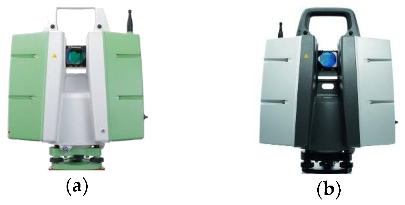
2.1. TLS Instruments
2.2. Study Area
2.3. Leaf Sampling
2.4. Leaf Samples Processing and Biochemistry Measurements
2.5. TLS Point-Cloud Processing
3. Results
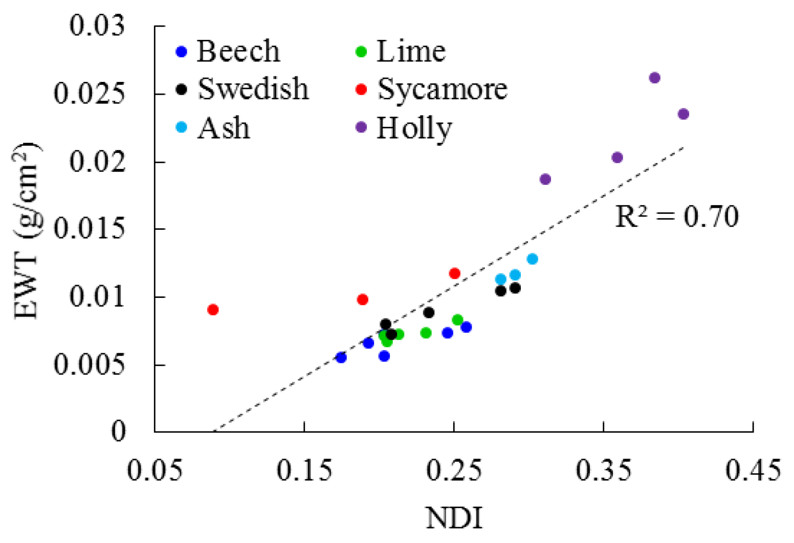
3.1. Leaf Level
3.2. Canopy Level
3.3. Temporal Change in EWT
3.4. EWT Vertical Profiles
4. Discussion
4.1. Leaf Level
4.2. Canopy Level
4.3. EWT Vertical Profiles
5. Conclusions
Author Contributions
Funding
Acknowledgments
Conflicts of Interest
References
- Schär, C.; Vidale, P.L.; Lüthi, D.; Frei, C.; Häberli, C.; Liniger, M.A.; Appenzeller, C. The role of increasing temperature variability in European summer heatwaves. Nature 2004, 427, 332. [Google Scholar] [CrossRef] [PubMed]
- Allen, C.D.; Breshears, D.D.; McDowell, N.G. On underestimation of global vulnerability to tree mortality and forest die-off from hotter drought in the anthropocene. Ecosphere 2015, 6, 1–55. [Google Scholar] [CrossRef]
- García-Herrera, R.; Díaz, J.; Trigo, R.M.; Luterbacher, J.; Fischer, E.M. A review of the european summer heat wave of 2003. Crit. Rev. Environ. Sci. Technol. 2010, 40, 267–306. [Google Scholar] [CrossRef]
- Stott, P.A.; Stone, D.A.; Allen, M.R. Human contribution to the European heatwave of 2003. Nature 2004, 432, 610. [Google Scholar] [CrossRef] [PubMed]
- Vogel, M.M.; Zscheischler, J.; Wartenburger, R.; Dee, D.; Seneviratne, S.I. Concurrent 2018 hot extremes across northern hemisphere due to human-induced climate change. Earth’s Future 2019, 7, 692–703. [Google Scholar] [CrossRef]
- Mitchell, D.; Kornhuber, K.; Huntingford, C.; Uhe, P. The day the 2003 European heatwave record was broken. Lancet Planet. Health 2019, 3, e290–e292. [Google Scholar] [CrossRef]
- Ceccato, P.; Flasse, S.; Tarantola, S.; Jacquemoud, S.; Grégoire, J.-M. Detecting vegetation leaf water content using reflectance in the optical domain. Remote Sens. Environ. 2001, 77, 22–33. [Google Scholar] [CrossRef]
- Jarvis, P.G.; McNaughton, K. Stomatal control of transpiration: Scaling up from leaf to region. In Advances in Ecological Research; Elsevier: London, UK, 1986; Volume 15, pp. 1–49. [Google Scholar]
- Farquhar, G.D.; Sharkey, T.D. Stomatal conductance and photosynthesis. Annu. Rev. Plant Physiol. 1982, 33, 317–345. [Google Scholar] [CrossRef]
- Bartlett, M.K.; Klein, T.; Jansen, S.; Choat, B.; Sack, L. The correlations and sequence of plant stomatal, hydraulic, and wilting responses to drought. Proc. Natl. Acad. Sci. USA 2016, 113, 13098–13103. [Google Scholar] [CrossRef] [PubMed]
- McDowell, N.G.; Fisher, R.A.; Xu, C.; Domec, J.; Hölttä, T.; Mackay, D.S.; Sperry, J.S.; Boutz, A.; Dickman, L.; Gehres, N. Evaluating theories of drought-induced vegetation mortality using a multimodel–experiment framework. New Phytol. 2013, 200, 304–321. [Google Scholar] [CrossRef] [PubMed]
- Sepulcre-Cantó, G.; Zarco-Tejada, P.J.; Jiménez-Muñoz, J.; Sobrino, J.; De Miguel, E.; Villalobos, F.J. Detection of water stress in an olive orchard with thermal remote sensing imagery. Agric. For. Meteorol. 2006, 136, 31–44. [Google Scholar] [CrossRef]
- Yebra, M.; Chuvieco, E.; Riaño, D. Estimation of live fuel moisture content from modis images for fire risk assessment. Agric. For. Meteorol. 2008, 148, 523–536. [Google Scholar] [CrossRef]
- Clevers, J.G.P.W.; Kooistra, L.; Schaepman, M.E. Estimating canopy water content using hyperspectral remote sensing data. Int. J. Appl. Earth Obs. Geoinf. 2010, 12, 119–125. [Google Scholar] [CrossRef]
- Ceccato, P.; Gobron, N.; Flasse, S.; Pinty, B.; Tarantola, S. Designing a spectral index to estimate vegetation water content from remote sensing data: Part 1—Theoretical approach. Remote Sens. Environ. 2002, 82, 188–197. [Google Scholar] [CrossRef]
- Tucker, C.J. Remote sensing of leaf water content in the near infrared. Remote Sens. Environ. 1980, 10, 23–32. [Google Scholar] [CrossRef]
- Zarco-Tejada, P.J.; Rueda, C.A.; Ustin, S.L. Water content estimation in vegetation with modis reflectance data and model inversion methods. Remote Sens. Environ. 2003, 85, 109–124. [Google Scholar] [CrossRef]
- Hunt, J.E.; Rock, B. Detection of changes in leaf water content using near- and middle-infrared reflectance. Remote Sens. Environ. 1989, 30, 43–54. [Google Scholar]
- Hardisky, M.; Klemas, V.; Smart, M. The influence of soil salinity, growth form, and leaf moisture on the spectral radiance of. Spartina Alterniflora 1983, 49, 77–83. [Google Scholar]
- Gao, B.C. Ndwi—A normalised difference water index for remote sensing of vegetation liquid water from space. Remote Sens. Environ. 1996, 58, 257–266. [Google Scholar] [CrossRef]
- Peñuelas, J.; Filella, I.; Biel, C.; Serrano, L.; Save, R. The reflectance at the 950–970 nm region as an indicator of plant water status. Int. J. Remote Sens. 1993, 14, 1887–1905. [Google Scholar] [CrossRef]
- Chen, D.; Huang, J.; Jackson, T.J. Vegetation water content estimation for corn and soybeans using spectral indices derived from modis near-and short-wave infrared bands. Remote Sens. Environ. 2005, 98, 225–236. [Google Scholar] [CrossRef]
- Rodríguez-Pérez, J.R.; Riaño, D.; Carlisle, E.; Ustin, S.; Smart, D.R. Evaluation of hyperspectral reflectance indexes to detect grapevine water status in vineyards. Am. J. Enol. Vitic. 2007, 58, 302–317. [Google Scholar]
- Fensholt, R.; Sandholt, I. Derivation of a shortwave infrared water stress index from modis near-and shortwave infrared data in a semiarid environment. Remote Sens. Environ. 2003, 87, 111–121. [Google Scholar] [CrossRef]
- Yebra, M.; Dennison, P.E.; Chuvieco, E.; Riano, D.; Zylstra, P.; Hunt, E.R., Jr.; Danson, F.M.; Qi, Y.; Jurdao, S. A global review of remote sensing of live fuel moisture content for fire danger assessment: Moving towards operational products. Remote Sens. Environ. 2013, 136, 455–468. [Google Scholar] [CrossRef]
- Ali, A.M.; Darvishzadeh, R.; Skidmore, A.K.; Duren, I.V. Effects of canopy structural variables on retrieval of leaf dry matter content and specific leaf area from remotely sensed data. J. Sel. Top. Appl. Earth Obs. Remote Sens. 2016, 9, 898–909. [Google Scholar] [CrossRef]
- Eitel, J.U.H.; Vierling, L.A.; Long, D.S. Simultaneous measurements of plant structure and chlorophyll content in broadleaf saplings with a terrestrial laser scanner. Remote Sens. Environ. 2010, 114, 2229–2237. [Google Scholar] [CrossRef]
- Serrano, L.; Ustin, S.L.; Roberts, D.A.; Gamon, J.A.; Penuelas, J. Deriving water content of chaparral vegetation from aviris data. Remote Sens. Environ. 2000, 74, 570–581. [Google Scholar] [CrossRef]
- Baret, F.; Guyot, G. Potentials and limits of vegetation indices for lai and apar assessment. Remote Sens. Environ. 1991, 35, 161–173. [Google Scholar] [CrossRef]
- Jacquemoud, S.; Baret, F.; Andrieu, B.; Danson, F.; Jaggard, K. Extraction of vegetation biophysical parameters by inversion of the prospect+ sail models on sugar beet canopy reflectance data. Application to tm and aviris sensors. Remote Sens. Environ. 1995, 52, 163–172. [Google Scholar] [CrossRef]
- Kötz, B.; Schaepman, M.; Morsdorf, F.; Bowyer, P.; Itten, K.; Allgöwer, B. Radiative transfer modeling within a heterogeneous canopy for estimation of forest fire fuel properties. Remote Sens. Environ. 2004, 92, 332–344. [Google Scholar] [CrossRef]
- Ustin, S.L.; Roberts, D.A.; Pinzon, J.; Jacquemoud, S.; Gardner, M.; Scheer, G.; Castaneda, C.M.; Palacios-Orueta, A. Estimating canopy water content of chaparral shrubs using optical methods. Remote Sens. Environ. 1998, 65, 280–291. [Google Scholar] [CrossRef]
- White, K.; Pontius, J.; Schaberg, P. Remote sensing of spring phenology in northeastern forests: A comparison of methods, field metrics and sources of uncertainty. Remote Sens. Environ. 2014, 148, 97–107. [Google Scholar] [CrossRef]
- Eastman, J.; Sangermano, F.; Machado, E.; Rogan, J.; Anyamba, A. Global trends in seasonality of normalized difference vegetation index (ndvi), 1982–2011. Remote Sens. 2013, 5, 4799–4818. [Google Scholar] [CrossRef]
- Améglio, T.; Archer, P.; Cohen, M.; Valancogne, C.; Daudet, F.-A.; Dayau, S.; Cruiziat, P. Significance and limits in the use of predawn leaf water potential for tree irrigation. Plant. Soil 1999, 207, 155–167. [Google Scholar] [CrossRef]
- Wang, Q.; Li, P. Canopy vertical heterogeneity plays a critical role in reflectance simulation. Agric. For. Meteorol. 2013, 169, 111–121. [Google Scholar] [CrossRef]
- Kuusk, A. A two-layer canopy reflectance model. J. Quant. Spectrosc. Radiat. Transf. 2001, 71, 1–9. [Google Scholar] [CrossRef]
- Elsherif, A.; Gaulton, R.; Mills, J. Estimation of vegetation water content at leaf and canopy level using dual-wavelength commercial terrestrial laser scanners. Interface Focus 2018, 8, 59–69. [Google Scholar] [CrossRef]
- Zhu, X.; Wang, T.; Skidmore, A.K.; Darvishzadeh, R.; Niemann, K.O.; Liu, J. Canopy leaf water content estimated using terrestrial lidar. Agric. For. Meteorol. 2017, 232, 152–162. [Google Scholar] [CrossRef]
- Hancock, S.; Gaulton, R.; Danson, F.M. Angular reflectance of leaves with a dual-wavelength terrestrial lidar and its implications for leaf-bark separation and leaf moisture estimation. IEEE Trans. Geosci. Remote Sens. 2017, 55, 3084–3090. [Google Scholar] [CrossRef]
- Jacquemoud, S.; Baret, F. Prospect—A model of leaf optical-properties spectra. Remote Sens. Environ. 1990, 34, 75–91. [Google Scholar] [CrossRef]
- Kaasalainen, S.; Åkerblom, M.; Nevalainen, O.; Hakala, T.; Kaasalainen, M. Uncertainty in multispectral lidar signals caused by incidence angle effects. Interface Focus 2018, 8, 20170033. [Google Scholar] [CrossRef] [PubMed]
- Gaulton, R.; Danson, F.M.; Ramirez, F.A.; Gunawan, O. The potential of dual-wavelength laser scanning for estimating vegetation moisture content. Remote Sens. Environ. 2013, 132, 32–39. [Google Scholar] [CrossRef]
- Junttila, S.; Sugano, J.; Vastaranta, M.; Linnakoski, R.; Kaartinen, H.; Kukko, A.; Holopainen, M.; Hyyppä, H.; Hyyppä, J. Can leaf water content be estimated using multispectral terrestrial laser scanning? A case study with norway spruce seedlings. Front. Plant Sci. 2018, 9, 299. [Google Scholar] [CrossRef] [PubMed]
- Junttila, S.; Holopainen, M.; Vastaranta, M.; Lyytikäinen-Saarenmaa, P.; Kaartinen, H.; Hyyppä, J.; Hyyppä, H. The potential of dual-wavelength terrestrial lidar in early detection of ips typographus (L.) infestation–leaf water content as a proxy. Remote Sens. Environ. 2019, 231, 111264. [Google Scholar] [CrossRef]
- Elsherif, A.; Gaulton, R.; Shenkin, A.; Malhi, Y.; Mills, J. Three dimensional mapping of forest canopy equivalent water thickness using dual-wavelength terrestrial laser scanning. Agric. For. Meteorol. 2019, 276, 107627. [Google Scholar] [CrossRef]
- Elsherif, A.; Gaulton, R.; Mills, J. The potential of dual-wavelength terrestrial laser scanning in 3d canopy fuel moisture content mapping. In Proceedings of the ISPRS Geospatial Week 2019, Enschede, The Netherlands, 10–14 June 2019. [Google Scholar]
- Schneider, C.A.; Rasband, W.S.; Eliceiri, K.W. Nih image to imagej: 25 Years of image analysis. Nat. Methods 2012, 9, 671–675. [Google Scholar] [CrossRef]
- Danson, F.M.; Steven, M.D.; Malthus, T.J.; Clark, J.A. High-spectral resolution data for determining leaf water content. Int. J. Remote Sens. 1992, 13, 461–470. [Google Scholar] [CrossRef]
- Gara, T.W.; Darvishzadeh, R.; Skidmore, A.K.; Wang, T. Impact of vertical canopy position on leaf spectral properties and traits across multiple species. Remote Sens. 2018, 10, 346. [Google Scholar] [CrossRef]
- Chavana-Bryant, C.; Malhi, Y.; Wu, J.; Asner, G.P.; Anastasiou, A.; Enquist, B.J.; Caravasi, C.; Eric, G.; Doughty, C.E.; Saleska, S.R. Leaf aging of amazonian canopy trees as revealed by spectral and physiochemical measurements. New Phytol. 2016, 214, 1049–1063. [Google Scholar] [CrossRef]
- Arellano, P.; Tansey, K.; Balzter, H.; Boyd, D.S. Field spectroscopy and radiative transfer modelling to assess impacts of petroleum pollution on biophysical and biochemical parameters of the amazon rainforest. Environ. Earth Sci. 2017, 76, 217. [Google Scholar] [CrossRef]
- Buchanan-Wollaston, V. The molecular biology of leaf senescence. J. Exp. Bot. 1997, 48, 181–199. [Google Scholar] [CrossRef]
- Yuan, L.; Huang, Y.; Loraamm, R.W.; Nie, C.; Wang, J.; Zhang, J. Spectral analysis of winter wheat leaves for detection and differentiation of diseases and insects. Field Crop. Res. 2014, 156, 199–207. [Google Scholar] [CrossRef]
- Yilmaz, M.T.; Hunt, E.R., Jr.; Jackson, T.J. Remote sensing of vegetation water content from equivalent water thickness using satellite imagery. Remote Sens. Environ. 2008, 112, 2514–2522. [Google Scholar] [CrossRef]
- Champagne, C.M.; Staenz, K.; Bannari, A.; McNairn, H.; Deguise, J.-C. Validation of a hyperspectral curve-fitting model for the estimation of plant water content of agricultural canopies. Remote Sens. Environ. 2003, 87, 148–160. [Google Scholar] [CrossRef]
- Cheng, Y.-B.; Ustin, S.L.; Riaño, D.; Vanderbilt, V.C. Water content estimation from hyperspectral images and modis indexes in southeastern Arizona. Remote Sens. Environ. 2008, 112, 363–374. [Google Scholar] [CrossRef]
- Zhang, Y.; Zhu, H.; Yan, B.; Ou, Y.; Li, X. Vertical distribution and temporal variation of nitrogen, phosphorus and carbon in ditch sediment of Sanjiang plain northeast china. Fresenius Environ. Bull. 2013, 22, 2265–2272. [Google Scholar]
- Liu, S.; Peng, Y.; Wei, D.; Le, Y.; Li, L. Remote estimation of leaf and canopy water content in winter wheat with different vertical distribution of water-related properties. Remote Sens. 2015, 7, 4626–4650. [Google Scholar] [CrossRef]
- Aber, J.D. Foliage-height profiles and succession in northern hardwood forests. Ecology 1979, 60, 18–23. [Google Scholar] [CrossRef]
- Ellsworth, D.; Reich, P. Canopy structure and vertical patterns of photosynthesis and related leaf traits in a deciduous forest. Oecologia 1993, 96, 169–178. [Google Scholar] [CrossRef]
- Hikosaka, K. Leaf canopy as a dynamic system: Ecophysiology and optimality in leaf turnover. Ann. Bot. 2004, 95, 521–533. [Google Scholar] [CrossRef]
- Hirose, T.; Werger, M. Maximizing daily canopy photosynthesis with respect to the leaf nitrogen allocation pattern in the canopy. Oecologia 1987, 72, 520–526. [Google Scholar] [CrossRef] [PubMed]
- Chazdon, R.L.; Fetcher, N. Photosynthetic light environments in a lowland tropical rain forest in Costa Rica. J. Ecol. 1984, 553–564. [Google Scholar] [CrossRef]
- Herrera, C.M.; Bazaga, P. Epigenetic correlates of plant phenotypic plasticity: DNA methylation differs between prickly and nonprickly leaves in heterophyllous ilex aquifolium (aquifoliaceae) trees. Bot. J. Linn. Soc. 2013, 171, 441–452. [Google Scholar] [CrossRef]
- Lichtenthaler, H.K.; Buschmann, C.; Döll, M.; Fietz, H.J.; Bach, T.; Kozel, U.; Meier, D.; Rahmsdorf, U. Photosynthetic activity, chloroplast ultrastructure, and leaf characteristics of high-light and low-light plants and of sun and shade leaves. Photosynth. Res. 1981, 2, 115–141. [Google Scholar] [CrossRef] [PubMed]


| Index | Formula |
|---|---|
| NDII | (P820 − P1650)/(P820 + P1650) |
| NDWI | (P860 − P1240)/(P860 + P1240) |
| WI | (P900)/(P970) |
| MSI | (P1600)/(P820) |
| Leica P20 | Leica P50 | |
|---|---|---|
| Measurement type | time-of-flight | time-of-flight |
| Wavelength | 808 nm | 1550 nm |
| Maximum range | 120 m at 18% reflectivity | 1 km at 80% reflectivity |
| Beam diameter at exit | 2.8 mm | 3.5 mm |
| Beam diameter at 10 m | 4.8 mm | 5.8 mm |
| Beam diameter at 20 m | 6.8 mm | 8.1 mm |
| Beam divergence | 0.20 mrad | 0.23 mrad |
| August | October | |||
|---|---|---|---|---|
| EWT model | Validation | EWT model | Validation | |
| Swedish whitebeam | 5 | 5 | 5 | 5 |
| Ash | 3 | 5 | 5 | 4 |
| Beech | 6 | 5 | 5 | 5 |
| Holly | 4 | 5 | 4 | 5 |
| Sycamore | 3 | 4 | --- | --- |
| Lime | 5 | --- | --- | --- |
| Total number of leaf samples | 26 | 24 | 19 | 19 |
| August | October | |||
|---|---|---|---|---|
| Pooled EWT Model 1 | Pooled EWT Model 2 | Pooled EWT Model 1 | Pooled EWT Model 2 | |
| Swedish whitebeam | 23.4% | –2.2% | 17.8% | 6.3% |
| Ash | 25.5% | –4% | –4.2% | –5.6% |
| Beech | 56.2% | 12% | –17.6% | 7.3% |
| Holly | 1% | 4.4% (1) | 2.4% | 5.8% (1) |
| Sycamore | –46.7% | --- | --- | --- |
| Swedish Whitebeam | Ash | Beech | Holly | ||
|---|---|---|---|---|---|
| Actual EWT (g cm−2) from leaf sampling | August | 0.0092 | 0.0127 | 0.0068 | 0.0266 |
| October | 0.0108 | 0.0139 | 0.0082 | 0.0239 | |
| EWT change | 0.0016 | 0.0012 | 0.0014 | –0.0027 | |
| EWT change (%) | 17.4% | 9.5% | 20.6% | –10.2% | |
| Estimated EWT (g cm−2) from TLS | August | 0.0090 | 0.0121 | 0.0076 | 0.0268 |
| October | 0.0114 | 0.0131 | 0.0088 | 0.0245 | |
| EWT change | 0.0024 | 0.0010 | 0.0012 | –0.0023 | |
| EWT change (%) | 26.7% | 8.3% | 15.8% | –8.6% | |
© 2019 by the authors. Licensee MDPI, Basel, Switzerland. This article is an open access article distributed under the terms and conditions of the Creative Commons Attribution (CC BY) license (http://creativecommons.org/licenses/by/4.0/).
Share and Cite
Elsherif, A.; Gaulton, R.; Mills, J. Four Dimensional Mapping of Vegetation Moisture Content Using Dual-Wavelength Terrestrial Laser Scanning. Remote Sens. 2019, 11, 2311. https://doi.org/10.3390/rs11192311
Elsherif A, Gaulton R, Mills J. Four Dimensional Mapping of Vegetation Moisture Content Using Dual-Wavelength Terrestrial Laser Scanning. Remote Sensing. 2019; 11(19):2311. https://doi.org/10.3390/rs11192311
Chicago/Turabian StyleElsherif, Ahmed, Rachel Gaulton, and Jon Mills. 2019. "Four Dimensional Mapping of Vegetation Moisture Content Using Dual-Wavelength Terrestrial Laser Scanning" Remote Sensing 11, no. 19: 2311. https://doi.org/10.3390/rs11192311
APA StyleElsherif, A., Gaulton, R., & Mills, J. (2019). Four Dimensional Mapping of Vegetation Moisture Content Using Dual-Wavelength Terrestrial Laser Scanning. Remote Sensing, 11(19), 2311. https://doi.org/10.3390/rs11192311