Gaussian Process Graph-Based Discriminant Analysis for Hyperspectral Images Classification

Abstract

Dimensionality Reduction (DR) models are highly useful for tackling Hyperspectral Images (HSIs) classification tasks. They mainly address two issues: the curse of dimensionality with respect to spectral features, and the limited number of labeled training samples. Among these DR techniques, the Graph-Embedding Discriminant Analysis (GEDA) framework has demonstrated its effectiveness for HSIs feature extraction. However, most of the existing GEDA-based DR methods largely rely on manually tuning the parameters so as to obtain the optimal model, which proves to be troublesome and inefficient. Motivated by the nonparametric Gaussian Process (GP) model, we propose a novel supervised DR algorithm, namely Gaussian Process Graph-based Discriminate Analysis (GPGDA). Our algorithm takes full advantage of the covariance matrix in GP to constructing the graph similarity matrix in GEDA framework. In this way, more superior performance can be provided with the model parameters tuned automatically. Experiments on three real HSIs datasets demonstrate that the proposed GPGDA outperforms some classic and state-of-the-art DR methods.

1. Introduction

Hyperspectral images (HSIs) contain considerable different reflections of electromagnetic waves from visible light to near-infrared or even far-infrared [1,2]. This characteristic allows various ground objects to be discriminated based on HSIs with abundant information. Because of it, HSIs are widely used in astronomy [3], agriculture [4], biomedical imaging [5], geosciences [6] and military surveillance [7]. However, the abundant features in HSIs could lead to significant redundancy. When using traditional classification algorithms to distinguish the class/object of each pixels in HSIs, the curse of dimensionality or the so-called “Hughes Phenomenon” would occur [8]. Chang et al. found that up to 94% of the spectral bands can be brushed aside without affecting the classification accuracy [9]. Therefore, Dimensionality Reduction (DR), a pre-processing procedure which tries to discover low-dimensional latent features from high-dimensional HSIs, plays a vital role in HSIs data analysis and classification.

In general, DR methods can be divided into two categories: feature selection and feature extraction. The former attempts to select a small subset of bands from the original bands based on some criteria, while the latter tries to find a low-dimensional subspace embedded in high-dimensional observations [10]. As reviewed in [11], discovering optimal bands from large numbers of possible feature combinations by feature selection methods could be suboptimal, so we only focus on feature extraction based DR methods for HSIs instead of feature selection in this paper.

A variety of feature extraction based DR models have been introduced for HSIs data analysis over the past decades. They can be roughly divided into two categories: unsupervised and supervised DR techniques. Unsupervised DR methods try to find low-dimensional representations that could preserve the intrinsic structure of the high-dimensional observations without using labels, while supervised methods make use of the available labels to find low-dimensional and discriminant features. The most representative unsupervised DR algorithm could be Principal Component Analysis (PCA), which tries to use the linear model to project the observed data into low-dimensional space with maximal variances [12,13]. Based on PCA, various extensions have been proposed, such as Probabilistic PCA (PPCA), Robust PCA (RPCA), Sparse PCA, Tensor PCA, etc. [11,14,15,16,17,18]. However, the aforementioned algorithms belong to the linear DR methods. When dealing with nonlinear structures embedded into the high-dimensional HSIs data, PCA and its linear extensions could be unable to provide satisfactory performance. Therefore, many nonlinear DR methods have been introduced, among which manifold learning based DR models have been widely employed in HSIs data analysis [19,20,21].

Representative manifold learning based DR algorithms include Isometric Mapping (ISOMAP) [20], Locally Linear embedding (LLE) [19], Laplacian Eigenmaps (LE) [22], Local Tangent Space Alignment (LTSA) [23], etc. The idea behind these algorithms is to assume that the data lie along a low-dimensional manifold embedded in a high-dimensional Euclidean space, and to uncover this manifold structure [24] with different criteria. For example, ISOMAP, an extension of Multi-dimensional Scaling (MDS) [25], seeks a low-dimensional embedding that preserves geodesic distances of all the pairs of points. In LLE, each sample is reconstructed by a linear combination of its neighbors and then the corresponding low-dimensional representations that could preserve the linear reconstruction relationship in original space are solved. LE utilizes a similarity graph to represent the neighbor relationships of pairwise points in low-dimensional space. The local geometry via the tangent space is modeled in LTSA to learn the low-dimensional embedding. However, most of the manifold learning models encounter the so-called out-of-sample problem [26], which means it could be ineffective to find the low-dimensional representation corresponding to a new testing sample. An effective solution to this problem is to add a linear mapping that projects observed samples to low-dimensional subspace. For instance, Locality Preserving Projections (LPP) [27], Neighborhood Preserving Embedding (NPE) [28] and Linear Local Tangent Space Alignment (LLTSA) [29] are the linear extensions of LE, LLE and LTSA, respectively. In [30], a Graph Embedding (GE) framework has been proposed to unify these manifold learning methods on the basis of geometry theory. Recently, the representation-based algorithms have also been introduced to the GE framework to construct various similarity graphs [31]. For example, Sparse Representation (SR), Collaborative Representation (CR) and Low Rank Representation (LRR) [32] are utilized to constitute the sparse graph (${\ell }_1$ graph), collaborative graph (${\ell }_2$ graph) and low-rank graph, leading to Sparsity Preserving Projection (SPP) [33], Collaborative Representation based Projection (CRP) [34] and Low Rank Preserving Projections (LRPP) [35], respectively.

Nevertheless, the aforementioned algorithms are all unsupervised DR models, which means that extra labels available in HSIs data are not utilized. To take advantage of these label information, the unsupervised DR models can be extended to the supervised versions, which could improve the discriminative power of DR models [24]. In this line, Linear Discriminant Analysis (LDA), as the most well-known supervised DR model, attempts to improve the class-separability by maximizing the distance between heterogeneous samples and minimizing the distance between homogeneous samples [36]. However, LDA can only extract up to $c-1$ features with c being the number of label classes. Thus, Nonparametric Weighted Feature Extraction (NWFE) was proposed to tackle this problem by using the weighted mean to calculate the nonparametric scatter matrices which could obtain more than $c$-dimension features [37]. Other related works including Regularized LDA (RLDA) [38], Modified Fisher’s LDA (MFLDA) [39] and Supervised PPCA (SPPCA) [11,40] have been introduced for supervised HSIs feature extraction.

Apparently, the above supervised linear DR models may fail to discover the nonlinear geometric structure in HSIs data, resulting in unsatisfactory performance of DR models. Therefore, many supervised nonlinear DR methods have been introduced to find the complex geometric structure embedded in high-dimensional data. For example, Local Fisher Discriminant Analysis (LFDA) effectively combine the advantages of Fisher Discriminant Analysis (FDA) [41] and LPP by maximizing the between-class separability and minimizing the within-class distance simultaneously [42,43]. Local Discriminant Embedding (LDE) extends the concept of LDA to perform local discrimination [44,45]. Low-rank Discriminant Embedding (LRDE) learns the latent embedding space by maximizing the empirical likelihood and preserving the geometric structure [46]. Other related techniques include Discriminative Gaussian Process Latent Variable Model (DGPLVM) [47], Locally Weighted Discriminant Analysis (LWDA) [48], Multi-Feature Manifold Discriminant Analysis (MFMDA) [49], etc. Similarly, the representation based algorithms have also been introduced to supervised DR framework, such as Sparse Graph-based Discriminate Analysis (SGDA) [50], Weighted Sparse Graph-based Discriminate Analysis (WSGDA) [51], Collaborative Graph-based Discriminate Analysis (CGDA) [52], Laplacian regularized CGDA (LapCGDA) [53], Discriminant Analysis with Graph Learning (DAGL) [54], Graph-based Discriminant Analysis with Spectral Similarity (GDA-SS) [55], Local Geometric Structure Fisher Analysis (LGSFA) [56], Sparse and Low-Rank Graph-based Discriminant Analysis (SLGDA) [57], Kernel CGDA (KCGDA) [53], Laplacian Regularized Spatial-aware CGDA (LapSaCGDA) [58], etc. A good survey of these discriminant analysis models can be found in [31].

Although the graph embedding based DR methods are effective for extracting discriminative spectral features of HSIs data, these models are significantly affected by two factors: similarity graphs and model parameters. The similarity graph is the key for all the graph embedding models, while the performance of the models largely relies on the manual settings of model parameters, which is time-consuming and inefficient. Motivated by the nonparametric Gaussian Process (GP) model [59], we constitute the similarity graphs with GP in this paper. A Gaussian process is a type of continuous stochastic process, which defines a probability distribution over functions. With various covariance/kernel functions, GP can nonparametrically model complex and nonlinear mappings. Furthermore, all parameters of covariance functions typically termed hyperparameters can be learned automatically in GP. Inspired by the benefits of GP, we try to learn the similarity matrix in the graph embedding framework with GP. Specifically, the learned covariance matrix in GP is considered as the similarity graphs, giving rise to the Gaussian Process Graph based Discriminate Analysis (GPGDA), which could learn more efficient similarity graphs and avoid manually tuning parameters compared to existing algorithms. Experimental results on three HSIs datasets demonstrate that the proposed GPGDA can effectively improve the classification accuracy without time-consuming model parameters tuning.

The rest of the paper is organized as follows. In Section 2, we briefly review the related works, including the Gaussian Process (GP), Graph-Embedding Discriminate Analysis framework. The proposed Gaussian Process Graph-based Discriminate Analysis (GPGDA) is introduced in Section 3. Then, three HSIs datasets are used to evaluate the effectiveness of the proposed GPGDA in Section 4. Finally, a brief summary is given in Section 5.

2. Related Works

In this section, we briefly review the Gaussian Process and Graph-Embedding Discriminate Analysis framework. For the sake of consistency, we make use of the following notations throughout this paper: $X={[{\mathit{x}}_1,\dots ,{\mathit{x}}_N]}^T\in {\mathcal{R}}^{N\times D}$ are the original high-dimensional data with each sample ${\mathit{x}}_n\in {\mathcal{R}}^D$; $Y={[{\mathit{y}}_1,\dots ,{\mathit{y}}_N]}^T\in {\mathcal{R}}^{N\times 1}$ are the outputs where each sample ${\mathit{y}}_n\in \mathcal{R}$ (real values for regression tasks and discrete labels in $\{1,2,\dots ,C\}$ for classification tasks); $Z=[{\mathit{z}}_1,\dots ,{\mathit{z}}_N]\in {\mathcal{R}}^{d\times N}$ are the projected low-dimensional data with dimension $d\ll D$ and each ${\mathit{z}}_n$ corresponding to ${\mathit{x}}_n$ and ${\mathit{y}}_n$. For the sake of convenience, we further denote X as an $D\times N$ matrix, Y an $N\times 1$ vector and Z an $d\times N$ matrix.

2.1. Gaussian Process

Gaussian Process is typically used in Gaussian Process Regression (GPR), where we assume that each output sample ${\mathit{y}}_n$ is generated from the unknown function $\mathit{f}$ with independent and identically-distributed noise variables $ϵ$ with distributions $\mathcal{N}(0,{\sigma }^2)$, which is $\mathit{y}=\mathit{f}\left(\mathit{x}\right)+ϵ$. A Gaussian Process prior is placed over the latent function f, i.e., $\mathit{f}\sim \mathcal{N}\left(\mathit{f}\right|0,K_{XX})$, with the covariance matrix defined by the positive-semidefinite kernel function $K_{XX}=k(X,X|\theta )$. $\theta$ are the parameters of kernel function and typically termed as hyperparameters. The choice of kernel function and its hyperparameters settings determine the behavior of GP, which are fairly significant. With Bayesian theorem, the latent function $\mathit{f}$ can be marginalized analytically $P\left(Y\right|X,\theta )=\mathcal{N}\left(Y\right|0,K_{XX}+{\sigma }^{2}I)$. Generally, the parameter ${\sigma }^2$ of Gaussian noise can be easily merged into the covariance function with $K_Y=K_{XX}+{\sigma }^{2}I$. Thus, the hyperparameters of kernel function can be optimized by maximizing the log marginal likelihood

$$\begin{array}{c}\hfill logP\left(Y\right|X,\theta )=-\frac{1}{2}{Y}^T{K}_Y^{-1}Y-\frac{1}{2}log\left|K_Y\right|-\frac{n}{2}log2\pi .\end{array}$$

(1)

Considering a testing data point $\left\{({\mathit{x}}^{*},{\mathit{y}}^{*})\right\}$, the prediction distribution for a new test point ${\mathit{x}}^{*}$ can be calculated as follows

$$\begin{array}{c}\hfill {\mathit{f}}^{*}|{\mathit{x}}^{*},X,Y\sim \mathcal{N}(K_{{\mathit{x}}^{*}X}{(K_{XX}+{\sigma }^2\mathbf{I})}^{-1}Y,K_{{\mathit{x}}^{*}{\mathit{x}}^{*}}-K_{{\mathit{x}}^{*}X}{(K_{XX}+{\sigma }^2\mathbf{I})}^{-1}{K}_{X{\mathit{x}}^{*}})\end{array}$$

(2)

where Ks are the matrices of the covariance/kernel function values at the corresponding points X and/or ${\mathit{x}}^{*}$.

For the classification task with discrete outputs, active functions such as the sigmoid function $\tau \left(x\right)=1/(1+exp(-x\left)\right)$ as the likelihood model in $p(y_n=1|{\mathit{x}}_{\mathit{n}})=\tau \left(f\left({\mathit{x}}_{\mathit{n}}\right)\right)$ are typically introduced in Gaussian Process Classification (GPC) for binary classification. When making prediction, the predictive distributions over the $f^{*}=f\left({\mathit{x}}^{*}\right)$ and $y^{*}$ for a new test point ${\mathit{x}}^{*}$ are

$$\begin{array}{c}\hfill p\left({\mathit{f}}^{*}\right|{\mathit{x}}^{*},X,Y)=\int p\left({\mathit{f}}^{*}\right|{\mathit{x}}^{*},X,\mathit{f})p\left(\mathit{f}\right|X,Y)d\mathit{f}\\ \hfill p(y^{*}=1|{\mathit{x}}^{*},X,Y)=\int p\left(y^{*}\right|{\mathit{f}}^{*})p\left({\mathit{f}}^{*}\right|{\mathit{x}}^{*},X,Y)d{\mathit{f}}^{*}.\end{array}$$

(3)

It is worth noting that the two integrals become analytically intractable due to the non-Gaussianity of the logistic function $\tau \left(f\left({\mathit{x}}_{\mathit{n}}\right)\right)$, making it impossible to get the exact posterior in GPC. In such case, approximation techniques such as Laplace Approximation (LA), Expectation Propagation (EP), etc. are adopted to acquire the approximated GP posterior and conduct model optimization.

2.2. Graph-Embedding Discriminant Analysis

Many DR approaches have been proposed recently for HSIs feature extraction and classification, among which the Graph-Embedding Discriminant Analysis methods have shown promising performance [31]. Typically, Graph-Embedding Discriminant Analysis (GEDA) models try to find the projection matrix P in the mapping function ${\mathit{z}}_n=P^T{\mathit{x}}_n$ by preserving the similarities of samples in the original observation space. The objective function of GEDA can be denoted by

$$\begin{array}{cc}\hfill \tilde{P}& =\underset{P}{argmin}\sum _{i\ne j}\parallel {\mathit{z}}_i-{\mathit{z}}_j\parallel W_{ij}=\underset{P}{argmin}\sum _{i\ne j}\parallel P^T{\mathit{x}}_i-P^T{\mathit{x}}_j\parallel W_{ij}\hfill \\ \hfill & =\underset{P}{argmin}trace\left(P^{T}XL{X}^{T}P\right),s.t.P^{T}X{L}_p{X}^{T}P=I,\hfill \end{array}$$

(4)

where the similarity matrix W is an undirected intrinsic graph with each element $W_{ij}$ describing the similarity between samples ${\mathit{x}}_i$ and ${\mathit{x}}_j$, $L=T-W$ is the Laplacian matrix of graph W, T is the diagonal matrix with $T_{ii}={\sum }_{j=1}^N{W}_{ij}$ and $L_p$ is the constraint matrix defined to find a non-trivial solution of the objective function. Typically, $L_p$ is the diagonal matrix T for scale normalization and may also be the Laplacian matrix of penalty graph $W_p$. The intrinsic graph W characterizes intraclass compactness while the penalty graph $W_p$ describes interclass separability. By simply re-formulating the objective function, we can obtain

$$\begin{array}{c}\hfill \tilde{P}=\underset{P}{argmin}\frac{|P^{T}XL{X}^{T}P|}{|P^{T}X{L}_p{X}^{T}P|}.\end{array}$$

(5)

When $L_p$ is the Laplacian matrix of penalty graph $W_p$, Equation (5) is named as Marginal Fisher Analysis (MFA) [60]. The solution of Equation (5) can be easily obtained by solving the generalized eigenvalue decomposition problem

$$\begin{array}{c}\hfill XL{X}^{T}P=\lambda X{L}_p{X}^{T}P,\end{array}$$

(6)

where $P\in {\mathcal{R}}^{D\times d}$ is constructed by the eigenvectors corresponding to the d smallest eigenvalues. As we can see from the above formulations, the most significant step of GEDA is to build an intrinsic graph.

A popular approach that estimate the similarity between samples ${\mathit{x}}_i$ and ${\mathit{x}}_j$ is the heat kernel, which is utilized in unsupervised LPP

$$\begin{array}{c}\hfill W_{ij}=e^{-\frac{\parallel {\mathit{x}}_i-{\mathit{x}}_j{\parallel }^2}{r}},\end{array}$$

(7)

where $r>0$ denotes the local scaling of data samples. Different from unsupervised LPP that estimates the similarities of all the vertices, supervised discriminant analysis methods build the affinity matrix with label information, which will further improve the discriminative power. Thus, the similarity matrix W typically becomes a block-diagonal matrix

$$\begin{array}{c}\left[\begin{array}{cccc}{W}^1& & & \\ & W^2& & \\ & & \ddots & \\ & & & W^C\end{array}\right],\end{array}$$

(8)

where ${\left\{W^l\right\}}_{l=1}^C$ is the affinity matrix of size $n_l\times n_l$ only from the lth class.

Recently, representation based algorithms have been introduced to construct the within-class similarity matrix. For example, the sparse representation coefficients (${\ell }_1$ norm) is used to construct the similarity matrix $W^l=[{\mathit{w}}_1^l;{\mathit{w}}_2^l;\dots ;{\mathit{w}}_{n_l}^l]\in {\mathcal{R}}^{n_l\times n_l}$ in SGDA [50] ($n_l$ is the number of training data from the lth class). To reduce the computational complexity of SGDA, the collaborative representation (${\ell }_2$ norm) instead of sparse representation is used in CGDA [52]. Similarly, SLGDA [57], LapCGDA [53] and LapSaCGDA [58] were developed recently with different objective functions to construct the similarity matrices as follows,

$$\begin{array}{c}\begin{array}{c}\mathrm{SGDA}:{argmin}_{{\mathit{w}}_n^l}\parallel {\mathit{x}}_n^l-X_n^l{\mathit{w}}_n^l{\parallel }_2^2+\alpha {\parallel {\mathit{w}}_n^l\parallel }_1,\\ \mathrm{CGDA}:{argmin}_{{\mathit{w}}_n^l}\parallel {\mathit{x}}_n^l-X_n^l{\mathit{w}}_n^l{\parallel }_2^2+\alpha {\parallel {\mathit{w}}_n^l\parallel }_2,\\ \mathrm{SLGDA}:{argmin}_{W^l}\parallel X^l-X^l{W}^l{\parallel }_2^2+\alpha \parallel W^l{\parallel }_{*}+\beta {\parallel W^l\parallel }_1,\\ \mathrm{LapCGDA}:{argmin}_{{\mathit{w}}_n^l}\parallel {\mathit{x}}_n^l-X_n^l{\mathit{w}}_n^l{\parallel }_2^2+\alpha {\parallel {\mathit{w}}_n^l\parallel }_2+\beta {{\mathit{w}}_n^l}^T{H}_n{\mathit{w}}_n^l,\\ \mathrm{LapSaCGDA}:{argmin}_{{\mathit{w}}_n^l}\parallel {\mathit{x}}_n^l-X_n^l{\mathit{w}}_n^l{\parallel }_2^2+\alpha \parallel \Gamma {\mathit{w}}_n^l{\parallel }_2^2+\beta {\parallel \mathrm{diag}\left({\mathit{s}}_n\right){\mathit{w}}_n^l\parallel }_2^2+\gamma {{\mathit{w}}_{\mathit{n}}^{\mathit{l}}}^T{H}_n{\mathit{w}}_n^l,\end{array}\end{array}$$

(9)

where ${\mathit{x}}_n^l$ is a training sample from lth class, $X^l$ denotes all training samples from lth class, $X_n^l$ is $X^l$ excluding ${\mathit{x}}_n$, ${\parallel ·\parallel }_{*}$ in SLGDA indicates the nuclear norm, $H_n$ in LapCGDA and LapSaCGDA is the Laplacian matrix constructed by Equation (7), and $\Gamma$ and $\mathit{s}$ are similarly defined by ${\Gamma }_{ii}={\parallel x_n^l-x_i^l\parallel }_2$ and ${\mathit{s}}_n={\left[\mathrm{dist}((p_n,q_n),(p_i,q_i))\right]}^t$ with the pixel coordinate $(p_i,q_i)$ for samples in lth class $(i=1,2,\cdots ,n_l)$, respectively.

3. The Proposed Method

To effectively learn the similarity graphs without time-consuming parameters tuning in the Graph-Embedding Discriminant Analysis (GEDA) framework, the Gaussian Process Graph based Discriminant Analysis (GPGDA) method is proposed to address it. The GPGDA method makes use of the nonparametric and nonlinear GP model to learn the similarity/affinity matrix adaptively.

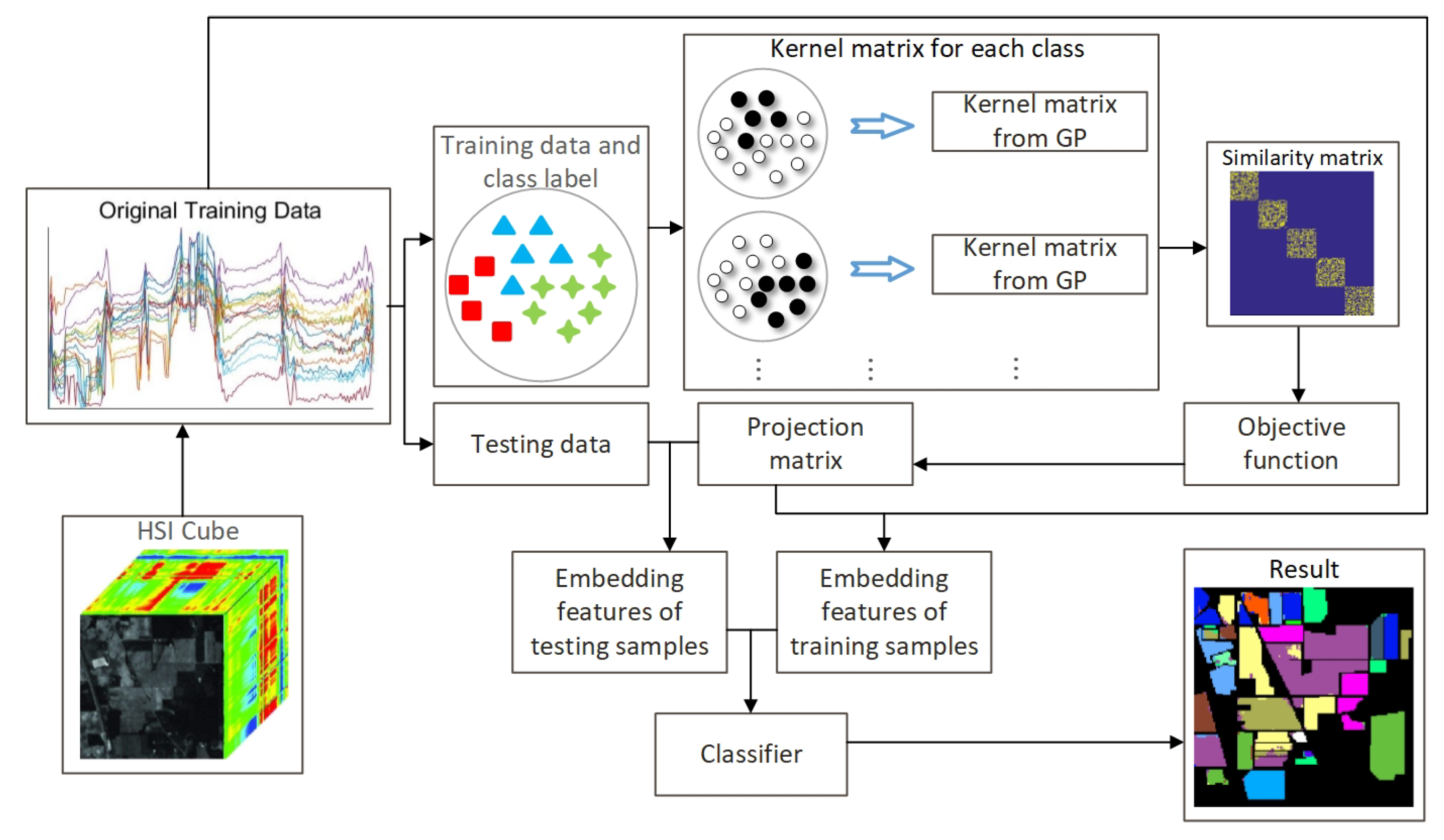
The flowchart of the proposed GPGDA method is shown in Figure 1. Firstly, the HSIs data will be divided into training and testing dataset randomly. Then, we try to construct the block-diagonal similarity matrix. Inspired by CGDA, we make use of GPR to model training samples from each class. To be specific, when we handle the training data from lth class, their labels are manually set to be 1 while the rest of the training data are labeled to be 0 conversely, which implicitly enforces interclass separability when learning the similarity graphs of each class. Thus, the learned similarity matrix should be more efficient than those from CGDA, KCGDA and other related algorithms. Subsequently, the similarity matrices of all classes are reassembled into the block-diagonal matrix, resulting a complete similarity matrix in the GEDA framework. Finally, the projection matrix can be acquired by solving the generalized eigenvalue decomposition problem and the dimension-reduced testing data can be obtained accordingly. To further measure the proposed method, the dimension-reduced training and testing data will be fed to different classifiers to get the prediction results.

From Section 2.1, we can learn that the convariance/kernel function is vital to GP since the corresponding kernel matrix measures the similarities between all pairs of samples. In view of this, kernel matrix in GP can be used to represent the similarity graph in GEDA framework. Because we want the intrinsic graph reflecting class-label information, it will be eventually expressed in the form of block-diagonal structure as in Equation (8). Here, we straightforwardly make use of GPR rather than GPC to model the high-dimensional training data with discrete labels, because time-consuming approximation methods in GPC could increase the model complexity. In addition, GPR is enough to model the class-specific training data.

Given a dataset $\mathcal{D}={\left\{({\mathit{x}}_i,{\mathit{y}}_i)\right\}}_{i=1}^N$, in which ${\mathit{x}}_i$ is a high-dimensional HSI sample and ${\mathit{y}}_i$ is the corresponding label. First, to efficiently learn the similar matrix, we set the label of training samples from lth class to be 1 while the rest are 0. The new binary labels can be denoted by $T={\left\{{\mathit{t}}_i\right\}}_{i=1}^N({\mathit{t}}_i\subset \{0,1\})$. Then, let us model the mapping from ${\mathit{x}}_i$ to ${\mathit{t}}_i$ with nonlinear GPR,

$$\begin{array}{c}\hfill P\left(T\right|X,\theta )=\mathcal{N}\left(T\right|0,K_T)\end{array}$$

(10)

The optimal hyperparameters $\theta$ of specific kernel function can be automatically estimated by optimizing the GPR objective function in Equation (1) with gradients based optimization algorithms. With the optimal hyperparameters, we could obtain the corresponding kernel matrix as follows,

$$\begin{array}{c}\hfill K_T=K(X^l,X^{\prime }|\theta ),\end{array}$$

(11)

where $X^l={\left\{{\mathit{x}}_n^l\right\}}_{n=1}^{n_l}$ are the training samples from lth class with the number of the class-specific data $n_l$, and ${\mathit{x}}^{\prime }$ denotes training data from other categories.

At this moment, we only care about training samples from lth class, which have been labeled to be 1, so we choose the $n_l\times n_l$ block from the kernel matrix, which corresponds to the samples from lth class in order to form the similarity matrix $W^l$. Once we have repeatedly obtained all the class-specific similarity matrix $W^l(l=1,\dots ,C)$ by GPR, the block-diagonal matrix W in Equation (8) can be simply constructed

$$\begin{array}{c}\hfill W=\mathrm{diag}(W^1,W^2,\dots ,W^C)\mathrm{with}{W}^l=\left[\begin{array}{ccc}k({\mathit{x}}_1^l,{\mathit{x}}_1^l)& \cdots & k({\mathit{x}}_1^l,{\mathit{x}}_{n_l}^l)\\ ⋮& \ddots & ⋮\\ k({\mathit{x}}_{n_l}^l,{\mathit{x}}_1^l)& \cdots & k({\mathit{x}}_{n_l}^l,{\mathit{x}}_{n_l}^l)\end{array}\right]\end{array}$$

(12)

Finally, based on the GEDA framework, it is easy to solve the optimal projection matrix P by solving the eigenvalue decomposition in Equation (6).

The complete GPGDA algorithm is outlined in Algorithm 1. To boost the performance of the models, we preprocess the HSIs data by a simple average filtering initially.

Algorithm 1 GPGDA for HSIs dimensionality reduction and classification.

Input: High-dimensional training samples $X\in {\mathcal{R}}^{D\times N}$, training ground truth $y\in {\mathcal{R}}^N$, pre-fixed latent dimensionality d, and testing pixels $X^{*}\in {\mathcal{R}}^{D\times M}$, testing ground truth $y^{*}\in {\mathcal{R}}^M$. Output: s = {$Acc$, P}. 1: Preprocess all the training and testing data by average filtering; 2: Estimate the hyperparameters’ set $\theta$ of kernel function by Equation (1); 3: Evaluate the similarity matrix W by Equation (11) and Equation (12); 4: Evaluate the optimal projection matrix P by solving the eigenvalue decomposition in Equation (6); 5: Evaluate low-dimensional features for all the training and testing data by ${\mathit{z}}_n=P^T{\mathit{x}}_n$; 6: Perform KNN/SVM in low-dimensional feature space and return classification accuracy $Acc$; 7: returns

As for the model complexity, since only small-scale training data are considered, we do not make use of the approximation methods such as Fully Independent Training Conditional (FITC) model [59] for GPR. Therefore, the time complexity of the proposed GPGDA is $\mathcal{O}\left(C{n_l}^3\right)$ where C is the number of the discrete classes and $n_l$ is the maximum number of samples in each class. By comparison, other discriminant analysis based methods such as CGDA and LapCGDA are with $\mathcal{O}\left(C{n_l}^3\right)$ as well because there are matrix inversion operation. Thus, the proposed GPGDA does not increase the model complexity theoretically.

4. Experiments

We validated the effectiveness of the proposed GPGDA for HSI feature extraction and classification by comparing with SPPCA, NWFE, DGPLVM, SLGDA, LapCGDA, KCGDA and LGSFA on three typical HSIs datasets. In addition, the traditional Support Vector Machine (SVM) and Convolutional Neural Network (CNN) [61] were applied in the original high-dimensional spectral feature space for comparison. K-Nearest Neighbors (KNN) with Euclidean distance and SVM with Radial Basis Function (RBF) kernel were adopted as classifiers in the learned low-dimensional space to verify all the DR models in terms of the classification Overall Accuracy (OA), the classification Average Accuracy (AA) and the Kappa Coefficient (KC). The parameter K in KNN was set to 5. The optimal parameters of kernel in SVM were selected by grid searching within a given set $\{{10}^{-6},{10}^{-5},\dots ,{10}^4\}$. The architecture of CNNs for each dataset is shown in

Table 1. Architecture of the CNN.

No.	Convolution	Batch Normalization	Rectified Linear Unit	Pooling	Stride	Dropout
1	$1\times 1\times 32$	YES	YES	$2\times 2$	2	NO
2	$5\times 5\times 48$	YES	YES	$2\times 2$	2	50%
3	$4\times 4\times 64$	NO	YES	$2\times 2$	2	50%

based on the experiments settings in [61]. For a fair comparison, all the data were preprocessed by average filtering with a $7\times 7$ spatial window, which is a simple and efficient method for smoothing HSIs. Experiments to verify the effect of different window sizes were also conducted; please refer to the Supplementary Materials for details.

Firstly, the most suitable kernel in GPGDA was chosen from 18 kernels in the fast Gaussian process latent variable model toolbox (FGPLVM) (http://inverseprobability.com/fgplvm/index.html). The corresponding hyperparameters of each kernel can be learned automatically in the proposed GPGDA. The regularization parameters such as $\alpha ,\beta$ for DGPLVM, SLGDA, LapCGDA and KCGDA were selected by the grid search with a given set $\{{10}^{-6},{10}^{-5},\dots ,{10}^4\}$.

Table 2. Optimal parameters settings for DGPLVM, SLGDA, LapCGDA and KCGDA on three HSI datasets.

	IndianPines		PaviaU		Salinas
Model	$\mathit{\alpha }$	$\mathit{\beta }$	$\mathit{\alpha }$	$\mathit{\beta }$	$\mathit{\alpha }$	$\mathit{\beta }$
DGPLVM	1	—	100	—	100	—
SLGDA	100	1	10	10	10	10
LapCGDA	0.01	100	0.1	100	0.01	1
KCGDA	0.1	—	0.0001	—	100	—

displays the best parameter values for the above four DR models. Then, after obtaining the optimal kernel and its corresponding hyperparameters, we compared and chose the best dimensionality of each DR model in the range of 1–30 in terms of the classification accuracy based on SVM in the projected low-dimensional space. Finally, we further compared all the DR models on the selected optimal dimension when different numbers of training data were chosen. All the experiments were repeated ten times and the average results are reported with standard deviation (STD). All methods were tested on MATLAB R2017a using an Intel Xeon CPU with 2.50 GHz and 64G memory PC with Linux platform.

4.1. Data Description

Three popular HSIs datasets were selected in our experiments (http://www.ehu.es/ccwintco/index.php/Hyperspectral_Remote_Sensing_Scenes).

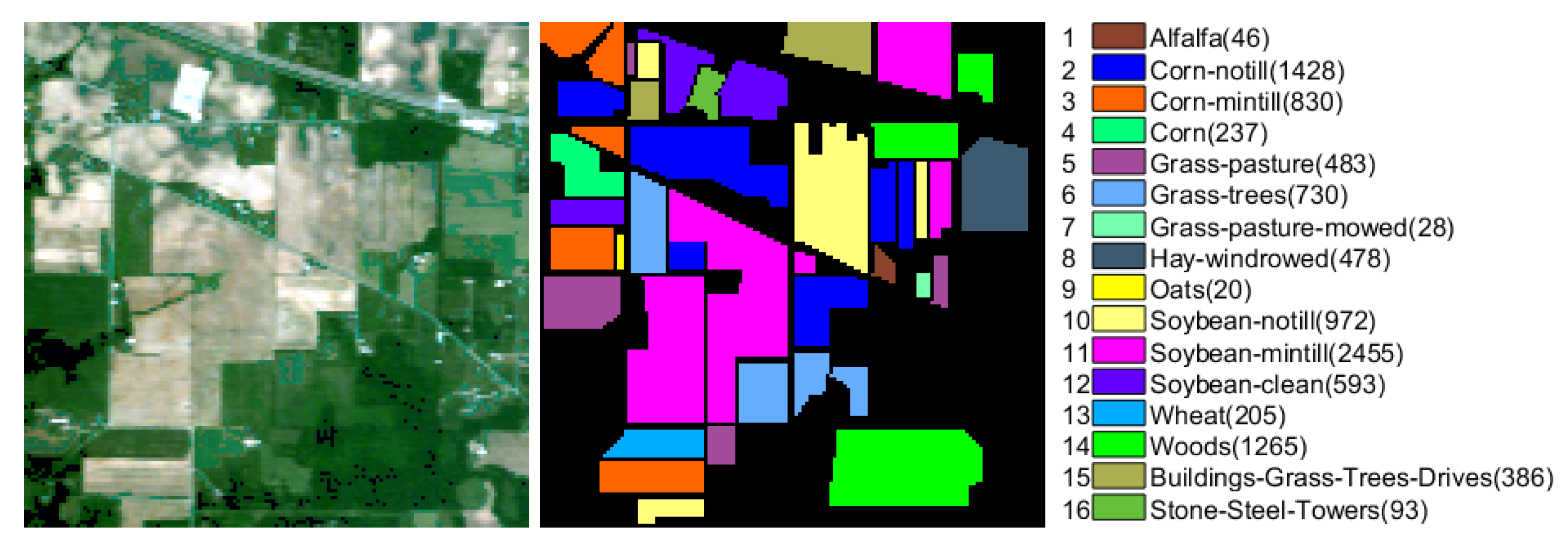
The Indian Pines scene (IndianPines) was captured by Airborne Visible/Infrared Imaging Spectrometer (AVIRIS) sensor over Northwest Indiana in 1992, which contains $145\times 145$ pixels and 200 spectral reflectance bands after discarding 24 bands affected by water absorption. Sixteen ground truth classes are discriminated in this dataset, and the False Color Composition (FCC) and Ground Truth (GT) are shown in Figure 2.

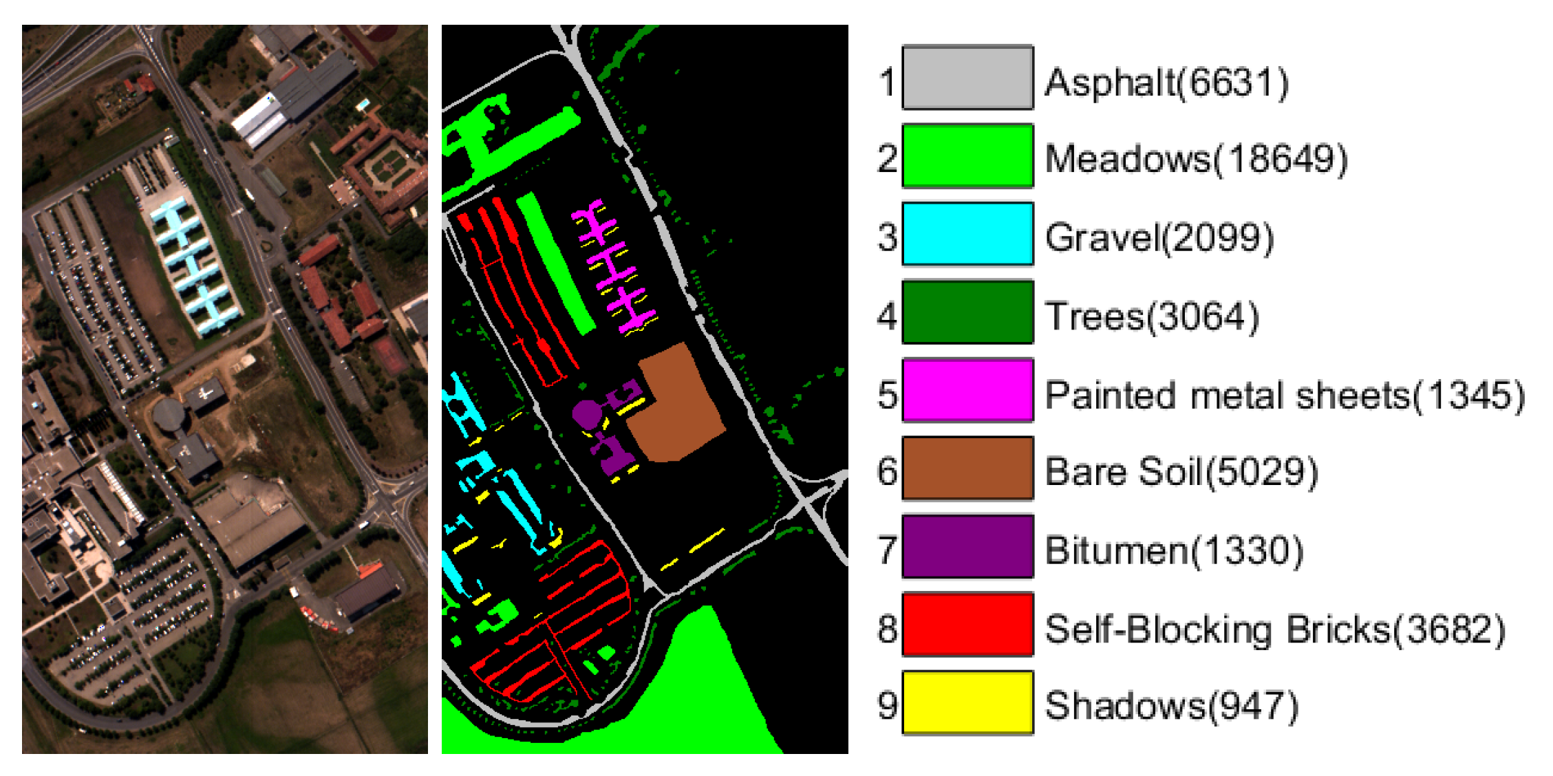
The University of Pavia scene (PaviaU) was gathered by Reflective Optics System Imaging Spectrometer (ROSIS-3) sensor over the University of Pavia, Italy in 2002. There are $610\times 340$ valid pixels with 103 spectral bands after removing some samples of the original scene containing no information. Nine ground truth classes are considered in this dataset, and the false color composition and ground truth are shown in Figure 3.

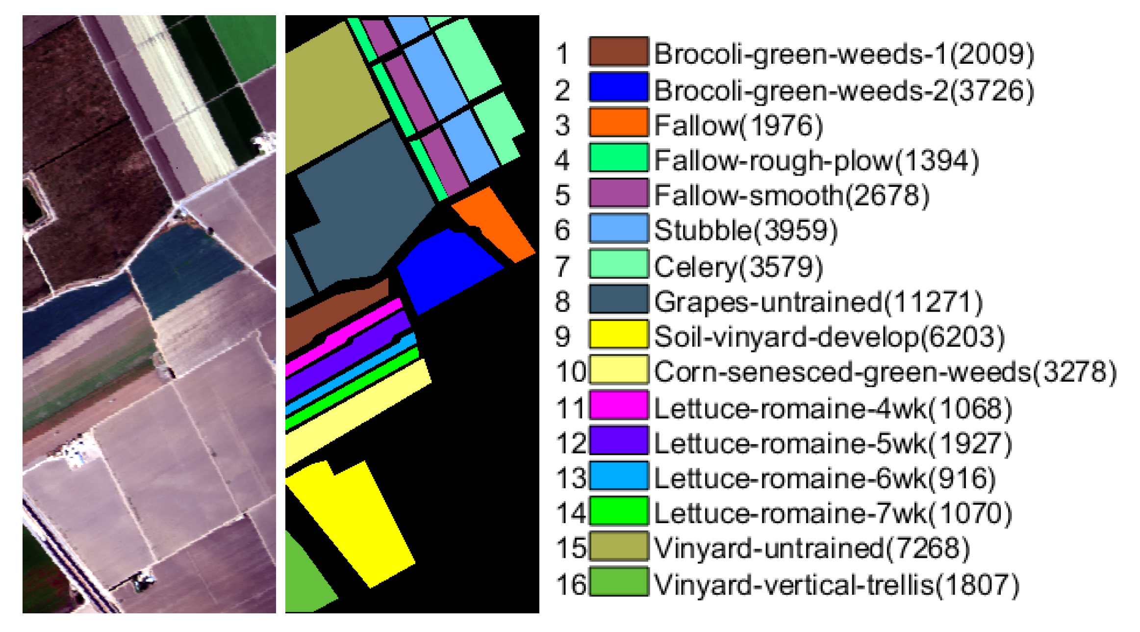
The Salinas Scene (Salinas) was collected by AVIRIS sensor over Salinas Valley, California in 1998, which consists of $512\times 217$ pixels with 224 spectral bands. Similar to Indian Pines scene, 20 water absorption and atmospheric effects bands are discarded, then the number of spectral bands becomes 204. Sixteen ground truth classes are labeled in this dataset, and the false color composition and ground truth are shown in Figure 4.

4.2. Sensitivity Analysis for Kernel

In this section, we mainly analyze the impact of all the 18 kernels in terms of OAs, because the type of kernel is the only thing that has to be manually selected in our proposed model. We randomly chose 30 samples from each class as training data and the remainder were testing data with the number of reduced dimensionality being 30.

Table 3. Classification accuracy based on the proposed GPGDA with 18 kernels on Indian Pines, University of Pavia and Salinas datasets.

	IndianPines		PaviaU		Salinas
Kernel	KNN	SVM	KNN	SVM	KNN	SVM
rbf	78.23 ± 1.99	89.66 ± 0.55	83.48 ± 1.42	93.98 ± 0.36	91.94 ± 1.14	94.97 ± 0.35
mlp	83.73 ± 2.97	89.18 ± 1.99	85.87 ± 1.22	93.68 ± 0.59	91.09 ± 1.54	94.62 ± 0.98
poly	83.27 ± 0.94	91.70 ± 0.69	84.07 ± 6.17	89.71 ± 2.52	92.55 ± 0.78	94.91 ± 0.72
lin	84.01 ± 0.60	91.32 ± 0.82	86.61 ± 1.83	93.84 ± 0.75	92.21 ± 0.51	95.06 ± 0.40
rbfard	79.13 ± 3.17	89.10 ± 0.97	81.26 ± 3.43	93.32 ± 0.87	90.41 ± 0.49	94.66 ± 0.33
mlpard	84.63 ± 1.83	90.54 ± 0.59	85.57 ± 1.74	93.67 ± 0.57	91.27 ± 1.52	94.49 ± 1.12
polyard	83.38 ± 1.71	91.51 ± 0.67	81.35 ± 7.84	87.57 ± 6.58	92.56 ± 0.75	94.96 ± 0.68
linard	85.15 ± 0.70	91.17 ± 1.00	87.29 ± 1.56	93.77 ± 0.54	92.28 ± 0.58	95.13 ± 0.48
matern32	79.95 ± 1.51	89.53 ± 0.73	75.65 ± 20.74	82.82 ± 23.13	92.37 ± 1.58	95.30 ± 0.56
matern52	80.60 ± 1.87	90.34 ± 0.50	81.47 ± 2.67	92.79 ± 0.75	92.80 ± 1.06	95.32 ± 0.25
rbfard2	79.95 ± 0.58	90.27 ± 0.62	77.34 ± 4.65	91.20 ± 0.99	92.87 ± 1.19	95.58 ± 0.06
sqexp	81.28 ± 2.62	90.19 ± 0.94	82.80 ± 3.13	93.20 ± 1.00	92.76 ± 1.00	95.39 ± 0.51
tensor	63.19 ± 2.05	85.54 ± 0.34	67.01 ± 0.86	90.96 ± 1.94	87.36 ± 0.57	93.22 ± 0.81
dexp	83.34 ± 1.42	91.71 ± 0.58	87.97 ± 1.41	93.88 ± 0.60	91.82 ± 1.86	95.18 ± 1.06
exp	64.03 ± 1.99	85.84 ± 0.32	67.57 ± 0.83	91.05 ± 1.87	87.52 ± 0.62	93.24 ± 0.83
gaussian	78.23 ± 1.99	89.66 ± 0.55	83.48 ± 1.42	93.98± 0.36	91.94 ± 1.14	94.97 ± 0.35
gg	78.48 ± 2.10	89.60 ± 0.60	82.85 ± 2.04	93.43 ± 1.09	92.43 ± 1.48	95.11 ± 0.37
gibbs	80.96 ± 2.48	90.24 ± 1.41	83.89 ± 3.70	93.41 ± 0.67	93.01 ± 0.80	95.36 ± 0.54

demonstrates the OAs based on the proposed GPGDA with different kernels on three HSIs datasets, where we can see that many kernels (up to 10 kernels on each dataset) could provide satisfactory results in terms of OAs in bold. Thus, choosing the best kernel function is not a big problem for our model. For the Indian Pines, University of Pavia and Salinas scenes, we have recommended ten kernels for each dataset with respect to the following experimental results. As for other HSI datasets that have not been studied in this paper, the kernels “dexp” and “lin” in the proposed GPGDA can be firstly considered as they could provide high accuracy for all the three datasets.

4.3. Experiments on the Indian Pines Data

Initially, an optimal kernel was selected for the proposed GPGDA based on the KNN and SVM classification results. The corresponding hyperparameters of each kernel could be learned via empirical Bayesian approach according to the training data. In this experiment, 30 samples were randomly chosen from each class as training data. When the number of training data in a certain category was less than 30, then 60% samples were chosen. For the fair comparison, the remaining data were split into the verification set (50%) and test set (50%). The optimal number of reduced dimensionality are chosen based on the verification set, and the reported results in Figure 5 are based on the test set.

As can be seen in Figure 5a,b, KNN and SVM based classification results from the proposed GPGDA with ten kernel functions are depicted. Here, we do not show all the results from 18 kernel functions because it could be chaos to plot 18 curves simultaneously. We only demonstrate ten kernels of poly, lin, mlpard, polyard, linard, matern52, rbfard2, sqexp, dexp and gibbs [59], which have better classification results than others. Although there are some differences for the ten kernels in terms of the KNN classification results, the classification results from SVM are similar, which means each one out of the ten kernels can be used efficiently. Since the ultimate goal of dimensionality reduction is classification, we only select the appropriate kernel based on SVM results, which are usually higher than KNN results. According to Figure 5b, kernel dexp is selected for the following experiments.

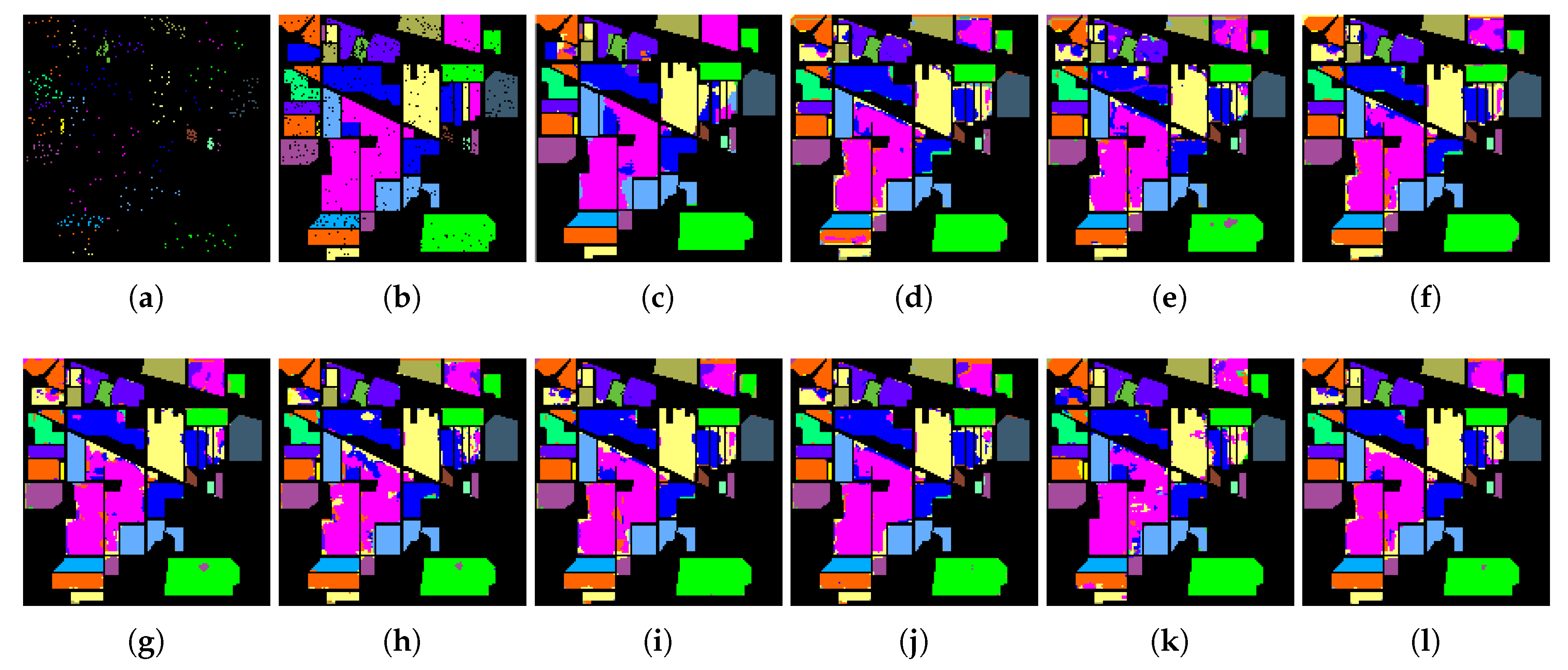
After setting the optimal kernel for GPGDA, we further conducted experiments to choose the best dimensionality of the projection space in terms of the OAs based on SVM. The optimal number of dimensionality of the projection space was selected from the range of 1–30. For the sake of fairness, the optimal regularization parameters in other DR models to be compared were set beforehand, as shown in the Table 2. It can be viewed in Figure 5c that, the optimal number of dimensionality for each DR model in Indian pines data is 30. It is also worth noting that, the OA of GPGDA surpasses other DR models on most dimensions, meaning that the learned low-dimensional features are very discriminatory.

Table 4. Classification results of CNN and different dimensionality reduction methods based on SVM on the Indian Pines data.

Class	Samples		DR Models
	Train	Test	CNN	SVM	SPPCA	NWFE	DGPLVM	SLGDA	LapCGDA	KCGDA	LGSFA	GPGDA
1	28	18	61.5 ± 14.5	54.1 ± 9.7	57.7 ± 16.7	65.8 ± 11.4	87.3 ± 11.7	93.0 ± 6.1	71.4 ± 14.8	65.9 ± 13.1	80.1 ± 13.7	83.8 ± 12.9
2	30	1398	91.1 ± 4.2	86.3 ± 5.2	77.9 ± 3.5	87.3 ± 4.1	86.4 ± 3.5	87.1 ± 4.8	90.8 ± 4.1	87.4 ± 4.4	89.6 ± 3.4	92.5 ± 3.8
3	30	800	81.0 ± 7.3	75.4 ± 5.5	82.1 ± 6.0	81.7 ± 4.8	84.1 ± 5.5	84.2 ± 3.4	82.9 ± 5.9	81.0 ± 3.6	81.1 ± 4.5	88.5 ± 4.3
4	30	207	87.0 ± 8.9	69.4 ± 7.2	75.7 ± 7.6	75.3 ± 7.3	81.6 ± 6.0	83.0 ± 9.0	81.4 ± 8.5	78.3 ± 8.5	85.5 ± 6.1	84.9 ± 8.1
5	30	453	95.4 ± 4.4	86.6 ± 8.1	83.5 ± 6.3	89.1 ± 6.5	92.7 ± 5.4	88.0 ± 7.9	91.5 ± 5.1	90.8 ± 5.8	95.1 ± 3.9	95.8 ± 3.0
6	30	700	87.3 ± 5.3	94.8 ± 2.9	98.3 ± 1.3	97.2 ± 1.9	98.0 ± 1.0	96.8 ± 1.3	98.6 ± 1.0	97.9 ± 1.2	97.1 ± 1.4	98.9 ± 0.9
7	17	11	80.7 ± 16.5	47.3 ± 22.6	61.5 ± 15.8	64.0 ± 32.8	82.9 ± 19.5	90.2 ± 8.5	72.1 ± 28.9	62.7 ± 31.4	84.6 ± 19.2	85.1 ± 18.4
8	30	448	94.9 ± 4.1	100.0 ± 0.0	100.0 ± 0.0	100.0 ± 0.0	99.6 ± 0.7	98.6 ± 4.3	100.0 ± 0.0	100.0 ± 0.0	99.8 ± 0.4	100.0 ± 0.1
9	12	8	47.8 ± 26.7	12.5 ± 2.5	48.7 ± 22.4	17.1 ± 4.6	61.1 ± 18.3	60.6 ± 22.7	38.0 ± 11.3	26.7 ± 8.2	34.5 ± 19.1	62.0 ± 13.4
10	30	942	84.1 ± 5.2	76.6 ± 5.5	75.1 ± 5.4	77.5 ± 6.5	77.8 ± 4.6	81.5 ± 6.8	78.1 ± 4.4	76.5 ± 5.5	80.8 ± 6.1	79.3 ± 5.2
11	30	2425	93.7 ± 2.9	92.5 ± 1.6	91.6 ± 2.6	94.0 ± 2.3	92.0 ± 3.0	93.8 ± 2.9	94.2 ± 1.9	92.8 ± 2.1	94.7 ± 1.3	94.8 ± 1.3
12	30	563	81.5 ± 5.7	78.6 ± 3.0	60.0 ± 5.1	81.6 ± 6.2	74.2 ± 7.0	84.2 ± 4.6	82.1 ± 5.5	81.0 ± 3.5	83.9 ± 5.9	83.9 ± 6.9
13	30	175	93.5 ± 5.7	94.1 ± 3.4	99.2 ± 1.3	98.2 ± 1.3	99.3 ± 1.5	98.4 ± 2.8	99.3 ± 1.0	99.0 ± 1.7	96.6 ± 2.6	99.6 ± 0.7
14	30	1235	97.1 ± 2.0	99.1 ± 0.5	98.6 ± 0.5	99.0 ± 0.8	98.6 ± 0.5	99.1 ± 0.7	98.9 ± 1.0	99.1 ± 0.7	98.9 ± 0.6	98.6 ± 0.6
15	30	356	66.0 ± 13.4	76.9 ± 3.7	74.6 ± 6.9	84.0 ± 4.4	83.5 ± 6.6	86.6 ± 4.5	85.4 ± 5.6	83.2 ± 6.3	89.7 ± 2.9	85.9 ± 5.5
16	30	63	74.3 ± 10.9	82.8 ± 8.0	89.2 ± 6.4	85.6 ± 8.3	89.3 ± 7.1	85.2 ± 10.4	86.6 ± 9.9	87.7 ± 8.2	79.1 ± 8.8	86.5 ± 8.7
AA(%)			82.2 ± 3.0	76.7 ± 1.7	79.6 ± 2.4	81.1 ± 2.6	86.8 ± 2.1	88.1 ± 2.6	84.5 ± 2.7	81.9 ± 2.8	85.7 ± 2.3	88.8 ± 1.9
OA(%)			89.2 ± 0.9	86.0 ± 1.0	83.5 ± 1.7	87.6 ± 1.6	88.5 ± 1.4	89.4 ± 1.3	89.4 ± 1.4	87.9 ± 1.2	89.8 ± 1.2	91.7 ± 0.6
KC			0.87 ± 0.01	0.77 ± 0.02	0.80 ± 0.02	0.81 ± 0.03	0.87 ± 0.02	0.88 ± 0.03	0.84 ± 0.03	0.82 ± 0.03	0.86 ± 0.02	0.89 ± 0.01
Runtime (in seconds)			38.41	1.31	0.17	18.18	848.85	24.42	2.48	3.18	4.35	112.32

illustrates the average classification accuracy of each class, the AAs, OAs, and KCs, as well as their STDs of eight DR models when dimensionality is 30 and classifier is SVM. Table 4 shows that the proposed GPGDA outperforms traditional CNN, SVM and other models in terms of the AA, OA and KC. Accordingly, Figure 6 tells us that classification maps from the proposed methods are more accurate than other contrastive approaches.

Finally, to verify the discriminating power of the proposed method even further, more classification experiments were conducted when different numbers of training data were randomly chosen: 10–60 samples were randomly chosen from each class, and the remainder were testing samples. For those classes with less samples, no more than 60% samples were randomly chosen.

Table 5. Classification results with different amounts of training data on the Indian pines data (OA ± STD (%)).

Classifier	DR Model	${\mathit{n}}_{\mathit{l}}=10$	${\mathit{n}}_{\mathit{l}}=20$	${\mathit{n}}_{\mathit{l}}=30$	${\mathit{n}}_{\mathit{l}}=40$	${\mathit{n}}_{\mathit{l}}=50$	${\mathit{n}}_{\mathit{l}}=60$
NN	SPPCA	54.26 ± 2.73	66.04 ± 1.42	70.77 ± 1.30	76.35 ± 1.30	78.98 ± 1.43	81.18 ± 0.89
	NWFE	62.62 ± 2.14	69.50 ± 1.75	74.89 ± 1.57	77.93 ± 1.55	79.88 ± 0.84	81.30 ± 1.06
	DGPLVM	68.09 ± 1.85	74.75 ± 2.14	78.40 ± 1.97	81.97 ± 1.50	84.86 ± 0.97	87.92 ± 1.16
	SLGDA	67.66 ± 1.49	76.75 ± 1.33	80.89 ± 1.88	84.59 ± 1.37	86.45 ± 1.06	88.28 ± 0.98
	LapCGDA	62.28 ± 31.48	67.31 ± 23.68	78.85 ± 1.79	81.09 ± 1.35	82.89 ± 1.22	83.90 ± 1.44
	KCGDA	57.35 ± 2.77	68.10 ± 1.86	72.79 ± 2.44	76.41 ± 2.04	79.33 ± 1.51	81.17 ± 1.09
	LGSFA	74.08 ± 1.86	84.34 ± 1.62	90.12 ± 1.28	92.63 ± 1.17	93.88 ± 0.99	95.15 ± 0.75
	GPGDA	66.78 ± 2.22	77.26 ± 2.09	82.50 ± 1.68	85.43 ± 1.63	88.09 ± 1.51	90.09 ± 0.86
SVM	SPPCA	71.80 ± 1.71	79.26 ± 1.51	83.53 ± 1.68	85.89 ± 1.12	87.80 ± 0.91	89.30 ± 0.73
	NWFE	76.50 ± 1.01	83.35 ± 1.49	87.62 ± 1.62	89.90 ± 0.82	91.33 ± 1.08	92.37 ± 0.83
	DGPLVM	76.70 ± 1.49	84.77 ± 1.03	88.52 ± 1.41	91.58 ± 0.75	93.10 ± 0.42	94.55 ± 0.46
	SLGDA	77.11 ± 1.29	85.17 ± 1.39	88.96 ± 0.93	91.23 ± 0.94	92.71 ± 0.65	94.17 ± 0.62
	LapCGDA	66.39 ± 37.19	77.18 ± 26.91	89.44 ± 1.36	91.04 ± 0.92	92.50 ± 1.06	93.61 ± 0.77
	KCGDA	74.74 ± 1.49	83.34 ± 1.04	87.85 ± 1.16	90.05 ± 0.88	91.89 ± 0.65	92.69 ± 0.60
	LGSFA	74.17 ± 1.94	84.05 ± 1.94	89.75 ± 1.16	92.59 ± 1.15	93.97 ± 0.94	95.37 ± 0.50
	GPGDA	79.87 ± 1.36	87.15 ± 1.21	91.71 ± 0.58	93.37 ± 0.68	94.80 ± 0.47	95.52 ± 0.34

shows that the OAs, AAs and KCs improve as the number of training samples increases for all methods. In addition, when classifier is KNN, LGSFA outperforms other DR models, followed by GPGDA. It is because LGSFA takes the intraclass neighbor reconstruction relationship of each training pixels into consideration, thus enhancing the class-separability of projected low-dimensional testing data. However, the local geometric structure is not utilized in GPGDA, thus it could be added in our future works. As for SVM classification accuracy, GPGDA demonstrates better OAs compared to other DR techniques. In general, the proposed GPGDA is capable of obtaining more discriminating features.

4.4. Experiments on the University of Pavia Data

To further demonstrate the effectiveness of the proposed algorithms, we chose the University of Pavia data to conduct experiments. Similarly, we firstly selected the optimal kernel and learned their corresponding hyperparameters for the proposed GPGDA. In this experiment, 30 training samples were randomly picked from each class while the remaining data were split into the verification set (50%) and test set (50%). The optimal number of reduced dimensionality was picked based on the verification set, and the reported results in Figure 7 are based on the test set.

According to Figure 7a,b, OAs based on KNN and SVM from the proposed GPGDA with ten kernel functions are illustrated. Considering the display effects, only ten well-performing kernels (rbf, mlp, lin, rgfard, mlpard, linard, dexp, gaussian, gg and gibbs) are shown. Similarly, there are some differences for the ten kernels in terms of the OAs based on KNN, but the classification results from SVM are almost coincidence with each other. Thus, choosing arbitrary kernel from these ten kernel functions would have little impact on the SVM classification results, indicating that selecting the best kernel function is not a troublesome problem for our model. In view of the fact that the OAs of dexp are the highest in both Figure 7a,b, we chose kernel dexp for the next experiments.

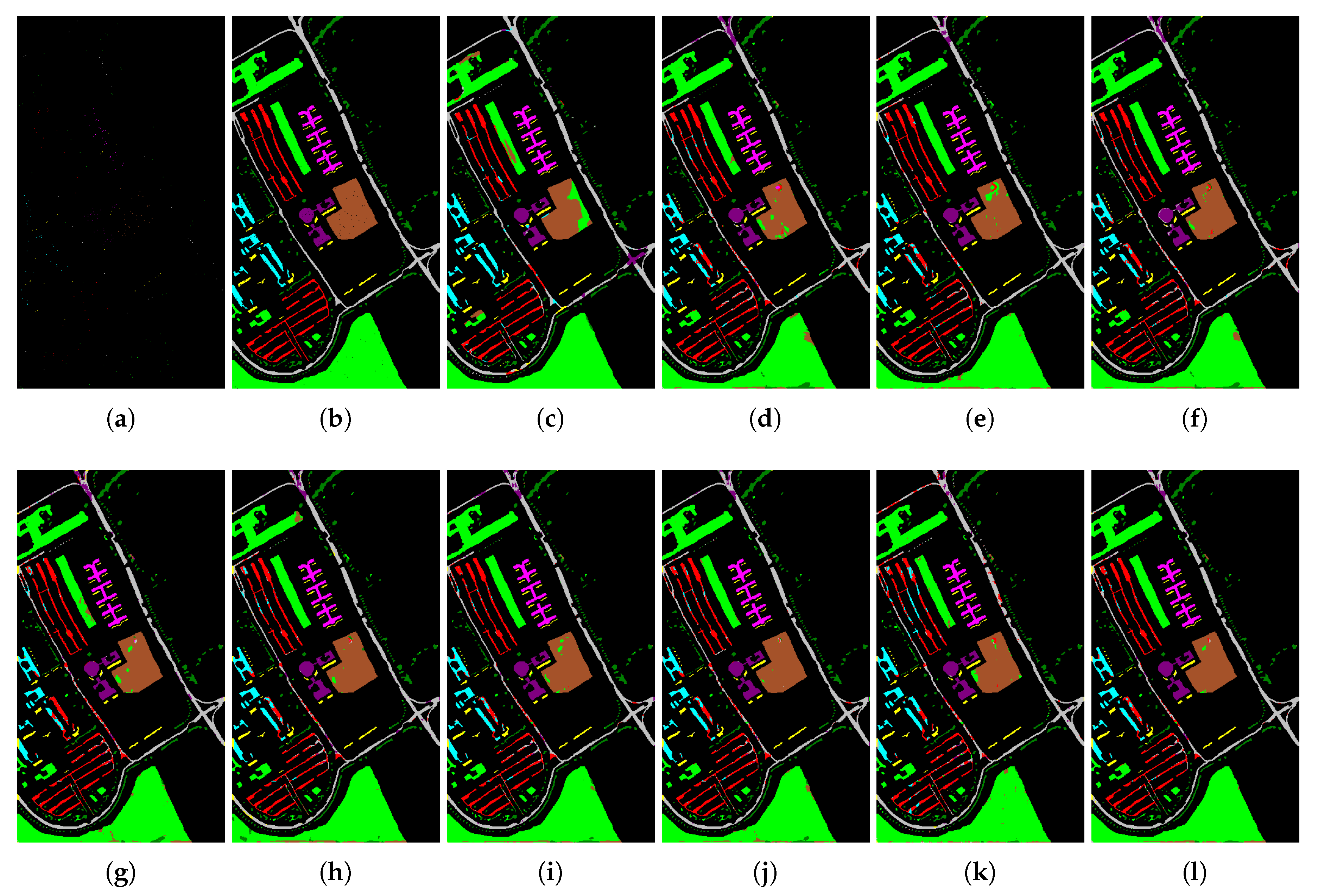
Once the optimal kernel for GPGDA was chosen, we chose the best dimensionality of the projection space in terms of the SVM results acquired in the low-dimensional space. All the experiments were conducted on low dimensions from 1 to 30. To be fair, the optimal regularization parameters in other contrastive DR models were determined via parameter sensitivity experiments, as shown in Table 2. Figure 7c shows that the proposed GPGDA is superior to other DR models in almost all the low-dimensional projection space. Moreover, the optimal number of dimensionality for each DR model in University of Pavia data is 30.

Table 6. Classification results of CNN and different DR methods based on SVM on the University of Pavia data.

Class	Samples		DR Models
	Train	Test	CNN	SVM	SPPCA	NWFE	DGPLVM	SLGDA	LapCGDA	KCGDA	LGSFA	GPGDA
1	30	6601	97.1 ± 2.2	92.2 ± 1.9	93.7 ± 2.5	93.0 ± 1.7	94.2 ± 1.1	92.8 ± 3.3	93.5 ± 1.6	92.7 ± 1.7	91.6 ± 1.9	94.3 ± 2.1
2	30	18619	96.1 ± 1.6	98.2 ± 0.7	97.9 ± 0.8	98.4 ± 0.6	98.1 ± 0.6	98.3 ± 0.5	98.7 ± 0.5	98.1 ± 1.0	97.4 ± 0.8	98.6 ± 0.4
3	30	2069	76.3 ± 9.3	84.5 ± 6.3	80.1 ± 7.9	85.1 ± 5.0	81.4 ± 8.2	81.8 ± 6.5	86.5 ± 5.0	85.1 ± 6.4	74.6 ± 6.0	86.5 ± 3.6
4	30	3034	97.3 ± 1.2	84.0 ± 7.7	90.1 ± 8.4	84.0 ± 9.9	85.3 ± 8.6	88.6 ± 4.5	86.6 ± 7.0	84.9 ± 7.4	93.1 ± 5.0	93.5 ± 1.3
5	30	1315	99.5 ± 0.5	98.7 ± 1.4	99.8 ± 0.2	99.8 ± 0.2	99.8 ± 0.1	98.9 ± 2.9	99.2 ± 1.9	99.3 ± 1.0	99.9 ± 0.1	98.7 ± 2.4
6	30	4999	76.7 ± 9.2	84.2 ± 4.4	82.5 ± 2.7	87.3 ± 4.4	88.9 ± 3.9	86.3 ± 5.0	87.5 ± 4.2	85.0 ± 4.8	84.4 ± 4.8	88.9 ± 5.1
7	30	1300	79.8 ± 8.4	79.2 ± 5.5	92.0 ± 6.2	82.1 ± 5.6	76.2 ± 2.2	83.5 ± 7.9	83.4 ± 6.7	80.0 ± 3.8	92.7 ± 4.9	87.6 ± 5.2
8	30	3652	89.8 ± 4.5	81.6 ± 3.5	84.4 ± 3.9	82.9 ± 4.3	82.7 ± 2.9	83.6 ± 3.2	84.6 ± 3.0	81.6 ± 3.4	78.9 ± 3.6	84.2 ± 3.2
9	30	917	95.5 ± 4.5	90.5 ± 5.5	87.0 ± 1.8	90.1 ± 5.7	88.8 ± 5.9	87.2 ± 7.4	89.0 ± 5.2	91.3 ± 5.3	92.1 ± 4.1	90.7 ± 4.1
AA(%)			89.8 ± 0.9	88.1 ± 1.1	89.7 ± 0.8	89.2 ± 0.8	88.4 ± 1.0	89.0 ± 1.7	89.9 ± 1.3	88.7 ± 0.8	89.4 ± 1.3	91.5 ± 0.6
OA(%)			90.4 ± 1.3	91.2 ± 0.9	92.5 ± 1.0	91.3 ± 1.18	92.6 ± 0.8	91.4 ± 1.5	91.8 ± 1.2	92.4 ± 0.8	91.2 ± 1.0	93.9 ± 0.6
KC			0.90 ± 0.01	0.88 ± 0.01	0.90 ± 0.01	0.89 ± 0.01	0.88 ± 0.01	0.89 ± 0.02	0.90 ± 0.01	0.89 ± 0.01	0.89 ± 0.01	0.91 ± 0.01
Runtime (in seconds)			23.61	1.82	0.22	3.45	483.93	19.37	1.4	0.9	1.81	62.82

displays the AAs, OAs, KCs and detailed classification accuracy for each class based on SVM when dimensionality is 30. In Table 6 we can see that GPGDA excels traditional CNN, SVM and other DR algorithms in terms of AA, OA and KC. Accordingly, the classification maps in Figure 8 give us a similar conclusion.

Finally, based on the optimal projection dimensionality, we further compared the discriminating power of the eight DR approaches by randomly selecting different number of pixels as training data. Here, 10–60 training samples were randomly chosen from each class, and the remainder were testing samples.

Table 7. Classification results with different amounts of training data on the University of Pavia data (OA ± STD (%)).

Classifier	DR Model	${\mathit{n}}_{\mathit{l}}=10$	${\mathit{n}}_{\mathit{l}}=20$	${\mathit{n}}_{\mathit{l}}=30$	${\mathit{n}}_{\mathit{l}}=40$	${\mathit{n}}_{\mathit{l}}=50$	${\mathit{n}}_{\mathit{l}}=60$
NN	SPPCA	63.69 ± 2.03	69.58 ± 1.79	73.73 ± 2.60	76.67 ± 3.27	79.91 ± 2.13	81.53 ± 2.57
	NWFE	63.59 ± 3.10	69.18 ± 3.34	73.53 ± 2.16	75.87 ± 2.55	79.51 ± 2.58	80.93 ± 2.25
	DGPLVM	69.98 ± 2.87	77.98 ± 3.07	82.93 ± 2.91	85.61 ± 1.62	87.63 ± 1.68	88.96 ± 1.11
	SLGDA	65.96 ± 4.16	78.56 ± 7.05	83.93 ± 2.98	86.45 ± 1.32	88.57 ± 1.98	88.73 ± 2.36
	LapCGDA	66.75 ± 5.45	71.74 ± 4.98	74.72 ± 3.36	78.65 ± 3.75	82.26 ± 3.03	84.16 ± 1.87
	KCGDA	58.76 ± 3.43	68.53 ± 2.49	72.91 ± 2.45	76.80 ± 2.22	80.48 ± 2.49	82.55 ± 2.01
	LGSFA	63.65 ± 4.59	81.80 ± 3.68	88.11 ± 1.13	89.57 ± 1.32	92.05 ± 1.26	92.98 ± 0.99
	GPGDA	65.03 ± 4.41	79.46 ± 2.16	87.97 ± 1.83	89.31 ± 2.17	91.95 ± 1.40	93.42 ± 0.47
SVM	SPPCA	85.34 ± 3.71	90.39 ± 2.46	92.51 ± 1.01	93.33 ± 1.06	93.96 ± 1.00	94.60 ± 0.75
	NWFE	85.06 ± 2.81	89.65 ± 1.94	91.30 ± 1.18	92.55 ± 1.04	93.56 ± 0.56	94.24 ± 0.75
	DGPLVM	84.24 ± 3.63	90.16 ± 1.21	92.63 ± 0.76	93.58 ± 0.71	94.67 ± 0.62	95.58 ± 0.59
	SLGDA	84.72 ± 3.03	89.03 ± 2.32	91.39 ± 1.53	92.19 ± 1.37	93.55 ± 1.10	93.65 ± 0.71
	LapCGDA	85.26 ± 2.81	90.47 ± 1.78	91.80 ± 1.24	92.94 ± 0.91	94.11 ± 0.44	94.84 ± 0.49
	KCGDA	83.53 ± 4.34	90.08 ± 2.13	92.40 ± 0.79	93.16 ± 0.86	94.10 ± 0.64	94.73 ± 0.60
	LGSFA	78.18 ± 3.57	85.76 ± 2.09	91.15 ± 1.04	92.84 ± 1.18	94.12 ± 0.86	95.32 ± 0.34
	GPGDA	87.78 ± 1.14	91.71 ± 0.28	93.88 ± 0.60	93.88 ± 1.45	95.52 ± 0.62	95.98 ± 0.52

shows that the OAs, AAs and KCs rise as the number of training samples increases for all methods. Specifically, LGSFA demonstrates comparative OAs based on KNN than the proposed GPGDA while GPGDA surpasses LGSFA and other methods in terms of the SVM classification results. This illustrates that GPGDA exceeds LGSFA, which preserves local geometric structure, in extracting discriminative features for HSIs data.

4.5. Experiments on the Salinas Data

Another challenging HSI data is the Salinas data. As we did before, we firstly chose the optimal kernel for the proposed GPGDA, in which the hyperparameters can be automatically learned via empirical Bayesian approach. Thirty training samples were randomly picked from each class in this experiment, while the remaining data were split into the verification set (50%) and test set (50%). The optimal number of reduced dimensionality and the reported results in Figure 7 are based on the verification set and the test set, respectively.

Figure 9a,b shows the KNN and SVM classification accuracy of the proposed GPGDA, respectively. For the sake of simplicity, ten better-performing kernels of all the kernels are demonstrated: lin, polyard, linard, matern32, matern52, rbfard2, sqexp, dexp, gg and gibbs. As in the experiments results for Indian Pines and University of Pavia datasets, slight differences are shown in Figure 9a,b, indicating that any of the ten kernels can be used efficiently. Since the SVM classification result of rbfard2 is slightly higher than others, kernel rbfard2 is finally picked.

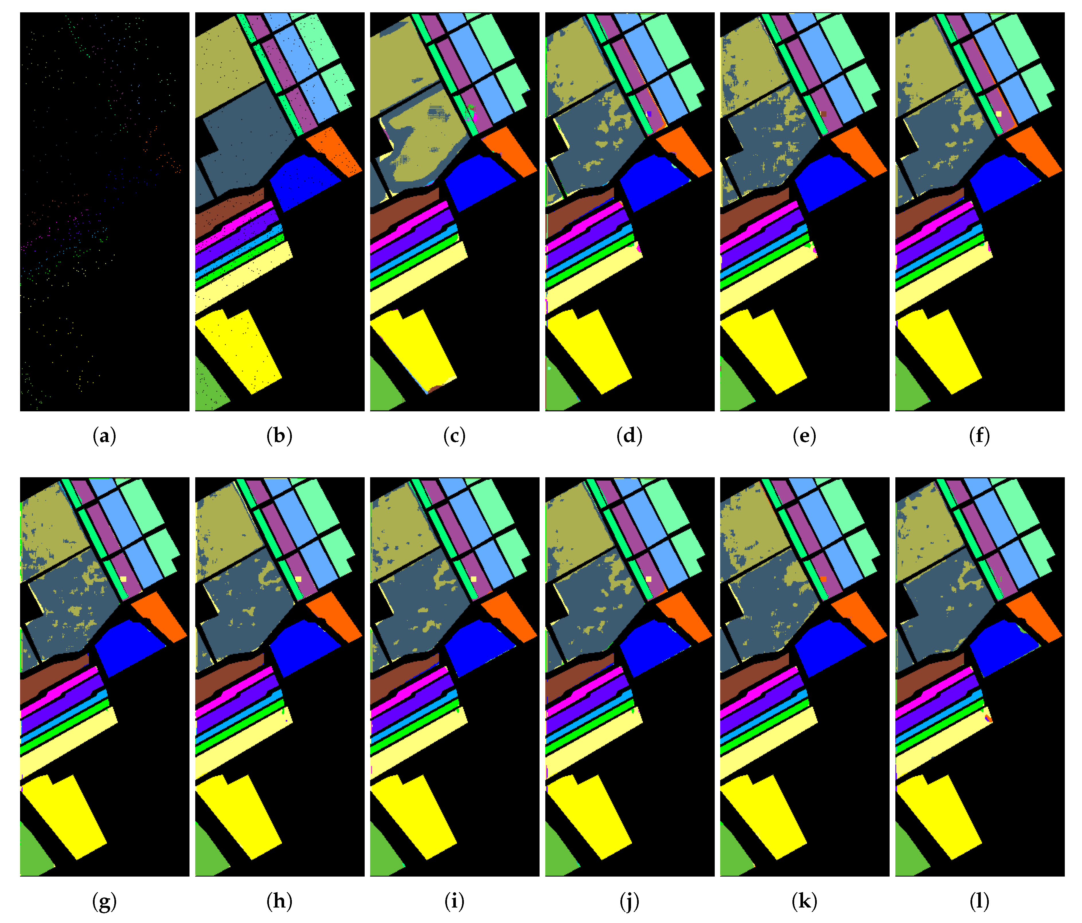
Having chosen the optimal kernel for GPGDA, the best dimensionality of the projection space can be obtained, as shown in Figure 9c, which describes the results based on SVM performed in the low-dimensional projection space. All the experiments were conducted on low-dimensional space in a range from 1 to 30. To make it fair, the best regularization parameters in other DR models were confirmed in advance. The optimal parameter values of other DR models on Salinas dataset are displayed in Table 2. Once again, the optimal number of dimensionality for all the DR models in Salinas data is 30.

Table 8. Classification results of CNN and different DR methods based on SVM on the Salinas data.

Class	Samples		DR Models
	Train	Test	CNN	SVM	SPPCA	NWFE	DGPLVM	SLGDA	LapCGDA	KCGDA	LGSFA	GPGDA
1	30	1979	91.2 ± 5.5	99.0 ± 1.4	99.7 ± 0.9	99.5 ± 1.2	99.8 ± 0.4	100.0 ± 0.0	99.9 ± 0.3	99.8 ± 0.6	100.0 ± 0.0	99.9 ± 0.1
2	30	3696	99.8 ± 0.5	99.2 ± 1.0	100.0 ± 0.0	99.3 ± 0.9	99.6 ± 0.3	99.7 ± 0.3	99.6 ± 0.6	99.6 ± 0.6	99.9 ± 0.2	99.7 ± 0.4
3	30	1946	99.6 ± 0.6	95.6 ± 1.8	98.6 ± 0.8	96.9 ± 2.6	99.9 ± 0.2	99.6 ± 0.5	98.0 ± 1.2	97.2 ± 1.1	99.2 ± 1.3	99.0 ± 0.8
4	30	1364	93.2 ± 3.1	94.1 ± 2.6	96.5 ± 1.8	97.6 ± 1.2	97.3 ± 1.6	97.8 ± 0.8	95.7 ± 2.2	96.7 ± 1.5	97.1 ± 1.4	98.1 ± 1.6
5	30	2648	98.6 ± 1.6	98.0 ± 0.7	98.9 ± 0.6	98.0 ± 0.9	98.7 ± 0.6	99.3 ± 0.4	98.8 ± 0.6	98.7 ± 0.7	99.2 ± 0.5	99.0 ± 0.3
6	30	3929	99.4 ± 0.9	100.0 ± 0.0	100.0 ± 0.0	99.7 ± 1.1	99.9 ± 0.1	99.9 ± 0.2	100.0 ± 0.0	100.0 ± 0.0	99.9 ± 0.4	100.0 ± 0.0
7	30	3549	98.9 ± 2.2	98.4 ± 0.9	99.5 ± 0.7	99.1 ± 1.0	99.8 ± 0.3	99.7 ± 0.5	99.1 ± 0.9	99.1 ± 0.9	100.0 ± 0.0	99.5 ± 0.7
8	30	11241	84.7 ± 10.4	90.1 ± 2.7	90.9 ± 1.9	91.6 ± 1.8	90.8 ± 2.2	91.7 ± 1.8	91.4 ± 1.9	91.9 ± 2.4	86.9 ± 2.6	93.9 ± 1.8
9	30	6173	99.7 ± 0.4	99.5 ± 0.4	99.4 ± 0.1	99.4 ± 0.3	99.6 ± 0.1	99.6 ± 0.1	99.6 ± 0.3	99.4 ± 0.4	99.6 ± 0.2	99.3 ± 0.5
10	30	3248	92.5 ± 5.1	89.7 ± 5.2	95.0 ± 2.6	92.0 ± 4.6	93.5 ± 2.8	90.2 ± 7.9	93.3 ± 2.9	92.2 ± 4.6	95.4 ± 2.0	92.2 ± 5.7
11	30	1038	95.4 ± 4.6	92.4 ± 2.6	98.2 ± 1.6	97.0 ± 3.8	99.0 ± 2.6	98.9 ± 1.8	97.8 ± 2.3	97.7 ± 2.9	99.9 ± 0.2	99.2 ± 1.1
12	30	1897	99.0 ± 1.8	95.8 ± 1.8	96.6 ± 4.8	96.8 ± 2.0	96.7 ± 4.8	98.5 ± 1.3	97.7 ± 1.9	97.2 ± 1.6	99.8 ± 0.3	98.3 ± 1.4
13	30	886	93.8 ± 7.0	94.9 ± 4.5	96.7 ± 2.9	97.8 ± 2.6	94.7 ± 4.9	96.8 ± 3.1	97.6 ± 3.2	97.5 ± 2.6	99.2 ± 1.3	99.0 ± 0.9
14	30	1040	95.2 ± 6.2	88.4 ± 7.5	95.9 ± 3.4	96.1 ± 2.0	95.5 ± 5.3	97.6 ± 2.3	97.5 ± 1.9	95.8 ± 4.1	99.1 ± 0.8	98.2 ± 1.0
15	30	7238	49.2 ± 10.4	81.8 ± 2.2	81.2 ± 4.8	82.9 ± 2.9	80.3 ± 4.0	81.7 ± 3.9	83.2 ± 2.7	82.6 ± 2.9	80.1 ± 2.8	85.5 ± 2.8
16	30	1777	99.2 ± 1.7	92.9 ± 6.5	96.2 ± 6.8	93.7 ± 7.2	95.0 ± 5.0	96.8 ± 3.8	94.4 ± 3.5	94.1 ± 7.3	99.9 ± 0.2	95.2 ± 7.5
AA(%)			93.1 ± 1.8	94.4 ± 0.8	96.5 ± 0.4	96.1 ± 0.5	96.2 ± 0.6	96.8 ± 0.6	96.5 ± 0.3	96.2 ± 0.5	97.2 ± 0.3	97.0 ± 0.4
OA(%)			84.2 ± 1.6	93.2 ± 0.6	94.7 ± 0.3	94.0 ± 0.6	94.1 ± 0.8	94.1 ± 0.8	94.2 ± 0.8	94.1 ± 0.5	94.2 ± 0.6	95.6 ± 0.1
KC			0.83 ± 0.02	0.94 ± 0.01	0.96 ± 0.00	0.96 ± 0.00	0.96 ± 0.01	0.97 ± 0.01	0.96 ± 0.00	0.96 ± 0.00	0.97 ± 0.00	0.97 ± 0.00
Runtime (in seconds)			41.24	2.05	0.41	20.87	985.72	25.37	2.28	3.39	4.77	233.12

displays the outperformance of GPGDA in terms of OA and KC. Accordingly, Figure 10 demonstrates that the classification map of GPGDA is more accurate than other methods.

Finally, based on the optimal projection dimensionality, we also conduct experiments when different amounts of training data were selected. In addition, 10–60 samples were randomly picked from all the labeled data, and the rest of data were the testing data.

Table 9. Classification results with different amounts of training data on the Salinas data (OA ± STD (%)).

Classifier	DR Model	${\mathit{n}}_{\mathit{l}}=10$	${\mathit{n}}_{\mathit{l}}=20$	${\mathit{n}}_{\mathit{l}}=30$	${\mathit{n}}_{\mathit{l}}=40$	${\mathit{n}}_{\mathit{l}}=50$	${\mathit{n}}_{\mathit{l}}=60$
NN	SPPCA	86.34 ± 3.67	89.47 ± 5.90	91.09 ± 4.45	92.08 ± 3.35	91.71 ± 3.34	92.74 ± 2.03
	NWFE	86.14 ± 2.13	88.57 ± 1.81	90.49 ± 0.74	91.08 ± 0.61	91.61 ± 0.32	92.24 ± 0.58
	DGPLVM	86.65 ± 1.86	89.25 ± 1.56	90.16 ± 0.89	91.94 ± 0.58	92.50 ± 0.62	92.98 ± 0.51
	SLGDA	85.45 ± 1.84	89.53 ± 1.85	91.60 ± 0.94	92.70 ± 0.62	93.05 ± 0.93	93.67 ± 0.71
	LapCGDA	86.34 ± 1.94	88.39 ± 2.25	91.02 ± 0.98	91.76 ± 1.10	91.83 ± 1.18	92.71 ± 1.48
	KCGDA	82.97 ± 1.56	86.60 ± 1.37	89.25 ± 0.62	90.16 ± 0.83	91.12 ± 0.63	91.94 ± 0.39
	LGSFA	90.33 ± 2.28	92.56 ± 1.53	94.33 ± 0.49	95.16 ± 0.55	95.34 ± 0.51	95.76 ± 0.51
	GPGDA	85.20 ± 2.05	89.83 ± 2.54	92.86 ± 1.20	93.56 ± 0.47	93.86 ± 0.72	94.52 ± 0.30
SVM	SPPCA	90.02 ± 1.18	92.92 ± 0.96	94.70 ± 0.34	95.06 ± 0.53	95.45 ± 0.37	95.91 ± 0.37
	NWFE	90.81 ± 0.74	92.85 ± 1.01	93.99 ± 0.56	94.62 ± 0.56	94.91 ± 0.46	95.31 ± 0.67
	DGPLVM	90.61 ± 1.41	93.01 ± 1.02	94.12 ± 0.83	95.45 ± 0.54	95.74 ± 0.42	96.13 ± 0.32
	SLGDA	90.72 ± 1.24	92.90 ± 1.25	94.13 ± 0.78	95.25 ± 0.60	95.64 ± 0.45	96.02 ± 0.34
	LapCGDA	91.30 ± 1.34	92.66 ± 1.25	94.15 ± 0.79	94.98 ± 0.87	95.43 ± 0.91	95.65 ± 0.91
	KCGDA	90.61 ± 1.32	92.79 ± 1.02	94.07 ± 0.54	94.85 ± 0.42	95.23 ± 0.48	95.60 ± 0.39
	LGSFA	91.49 ± 1.46	92.46 ± 1.37	94.17 ± 0.64	95.06 ± 0.56	95.48 ± 0.54	96.08 ± 0.43
	GPGDA	90.83 ± 2.18	93.23 ± 1.04	95.58 ± 0.06	96.07 ± 0.20	96.36 ± 0.37	96.77 ± 0.40

displays that the OAs, AAs and KCs keep an upward tendency as the number of training samples increases for all methods. Moreover, the OAs of GPGDA based on SVM are higher than other DR models, while LGSFA is superior to GPGDA in terms of KNN classification results because of the preserving local geometric structure. Generally, the experimental results in Table 9 corroborate the discriminating power of the proposed GPGDA.

5. Discussion

Based on above experimental results, we can provide the following discussions.

(i)

The proposed GPGDA outperforms SPPCA, NWFE, DGPLVM, SLGDA, LapCGDA, KCGDA and LGSFA in terms of OA, AA and KC based on SVM. As for the KNN classification results, LGSFA always takes the first place, but GPGDA is superior to other methods such as DGPLVM, SLGDA, and LapCGDA. The explanation could be that, although the learned similarity graph from GPGDA is more representative than that from other models, LGSFA preserves the intraclass neighbor reconstruction relationship in the objection function which considers the local manifolds. However, compared to other DR models of which regularization parameters needs be to be manually tuned via parameters sensitivity experiments, the only parameters of kernels in GPGDA can be learned automatically by gradients based optimization algorithms. Furthermore, the procedure of dividing the multi-class data into two classes enforces interclass separability when learning the kernel matrix from training data of each class.

(ii)

It is clear that KCGDA is a kernel based discriminant analysis method which combines the advantages of kernel and GEDA framework. However, it is quite difficult to set the optimal kernel parameters for KCGDA. Sometimes, KCGDA is even inferior to conventional CGDA because of the unsuitable parameters. DGPLVM is a GP based supervised DR model, but, unlike GPGDA, DGPLVM still has regularization parameters to be tuned. Thus, parameter sensitivity experiments should be carried out. By contrast, the proposed GPGDA outperforms the two models in terms of classification accuracy and automatic parameters tuning.

(iii)

The time complexity of GPGDA is $\mathcal{O}\left(C{n_l}^3\right)$, which is the same with other discriminant analysis based methods such as CGDA and LapCGDA. However, traditional discriminant analysis based methods are able to reach the close-form solutions straightforwardly, while the GPR in the proposed GPGDA is often optimized by gradients based optimization algorithms, which could be more time-consuming. Nevertheless, when the number of training samples is small, which is the case in HSIs classification, the training time can be short. In Table 4, Table 6 and Table 8, we report the running times of extracting the dimensionality reduced features with different algorithms on three HSIs datasets. It should be noted that, although the proposed GPGDA needs more running times than most contrastive DR models, the hyperparameters of GPGDA can be automatically learned, indicating that the time consumption for parameter sensitivity experiments with respect to other DR models can be saved significantly. Furthermore, if parallel computation is adopted to calculate the class-specific similarity matrix, the experiment time will be further greatly reduced.

(iv)

Deep Learning based methods such as Convolutional Neural Networks (CNN) can take spatial information into account while extracting spectral information from HSIs. Its performance can be sensitive to the depths and widths of the deep network. However, more layers means more parameters that needs to be learned. Due to the large number of learnable parameters, sufficient training samples are needed in CNNs to avoid the overfitting problem. Unfortunately, the lack of labeled training samples is a common bottleneck in HSI classification tasks, which could decrease the performance of CNN. By contrast, the only thing we need to select is the type of kernel in the proposed nonparametric model GPGDA, which could significantly outperform CNN especially in the small sample size scenario.

6. Conclusions

This paper introduces a novel supervised DR technique GPGDA for HSIs data based on the GEDA framework. The proposed GPGDA utilizes the kernel function in GP to calculate all the within-class matrices, and then constructs the block-diagonal intrinsic graph in the GEDA framework. Once we get the intrinsic graph, the optimal projection matrix can be evaluated based on the GEDA framework. To proves this, various experimental results illustrate that discriminative information for classification can be effectively extracted by the proposed DR methods. Our future work would focus on how to introduce the local geometric manifold structure of HSIs data into our GPGDA algorithm.

References

1. Solomon, J.; Rock, B. Imaging spectrometry for earth remote sensing. Science 1985, 228, 1147–1152. [Google Scholar]
2. Vane, G.; Duval, J.; Wellman, J. Imaging spectroscopy of the Earth and other solar system bodies. Remote Geochem. Anal. Elem. Mineral. Compos. 1993, 108, 121–166. [Google Scholar]
3. Hege, E.K.; O’Connell, D.; Johnson, W.; Basty, S.; Dereniak, E.L. Hyperspectral imaging for astronomy and space surviellance. Opt. Sci. Technol. 2004, 5159, 380–391. [Google Scholar]
4. Lacar, F.; Lewis, M.; Grierson, I. Use of hyperspectral imagery for mapping grape varieties in the Barossa Valley, South Australia. In Proceedings of the IEEE International Geoscience and Remote Sensing Symposium (IGARSS), Sydney, Australia, 9–13 July 2001; pp. 2875–2877. [Google Scholar]
5. Lu, G.; Fei, B. Medical hyperspectral imaging: A review. J. Biomed. Opt. 2014, 19, 010901. [Google Scholar] [CrossRef] [PubMed]
6. Kruse, F.A.; Boardman, J.W.; Huntington, J.F. Comparison of airborne hyperspectral data and EO-1 Hyperion for mineral mapping. IEEE Trans. Geosci. Remote Sens. 2003, 41, 1388–1400. [Google Scholar] [CrossRef]
7. Yuen, P.W.; Richardson, M. An introduction to hyperspectral imaging and its application for security, surveillance and target acquisition. Imaging Sci. J. 2010, 58, 241–253. [Google Scholar] [CrossRef]
8. Hughes, G. On the mean accuracy of statistical pattern recognizers. IEEE Trans. Inf. Theory 1968, 14, 55–63. [Google Scholar] [CrossRef]
9. Chang, C.I. Hyperspectral Data Exploitation: Theory and Applications; John Wiley & Sons: Hoboken, NJ, USA, 2007. [Google Scholar]
10. Jia, X.; Richards, J.A. Segmented principal components transformation for efficient hyperspectral remote-sensing image display and classification. IEEE Trans. Geosci. Remote Sens. 1999, 37, 538–542. [Google Scholar] [Green Version]
11. Xia, J.; Chanussot, J.; Du, P.; He, X. (Semi-) supervised probabilistic principal component analysis for hyperspectral remote sensing image classification. IEEE J. Sel. Top. Appl. Earth Obs. Remote Sens. 2014, 7, 2224–2236. [Google Scholar] [CrossRef]
12. Wold, S.; Esbensen, K.; Geladi, P. Principal component analysis. Chemom. Intell. Lab. Syst. 1987, 2, 37–52. [Google Scholar] [CrossRef]
13. Rodarmel, C.; Shan, J. Principal component analysis for hyperspectral image classification. Surv. Land Inf. Sci. 2002, 62, 115. [Google Scholar]
14. Bishop, C.M. Pattern Recognition and Machine Learning; Springer: Berlin/Heidelberg, Germany, 2006. [Google Scholar]
15. Candès, E.J.; Li, X.; Ma, Y.; Wright, J. Robust principal component analysis? J. ACM 2011, 58, 11. [Google Scholar] [CrossRef]
16. Zou, H.; Hastie, T.; Tibshirani, R. Sparse principal component analysis. J. Comput. Graph. Stat. 2006, 15, 265–286. [Google Scholar] [CrossRef]
17. Kutluk, S.; Kayabol, K.; Akan, A. Classification of Hyperspectral Images using Mixture of Probabilistic PCA Models. In Proceedings of the 24th European Signal Processing Conference, Budapest, Hungary, 29 August–2 September 2016; pp. 1568–1572. [Google Scholar]
18. Ren, Y.; Liao, L.; Maybank, S.J.; Zhang, Y.; Liu, X. Hyperspectral image spectral-spatial feature extraction via tensor principal component analysis. IEEE Geosci. Remote Sens. Lett. 2017, 14, 1431–1435. [Google Scholar] [CrossRef]
19. Roweis, S.T.; Saul, L.K. Nonlinear dimensionality reduction by locally linear embedding. Science 2000, 290, 2323–2326. [Google Scholar] [CrossRef] [PubMed]
20. Tenenbaum, J.B.; De Silva, V.; Langford, J.C. A global geometric framework for nonlinear dimensionality reduction. Science 2000, 290, 2319–2323. [Google Scholar] [CrossRef] [PubMed]
21. He, J.; Zhang, L.; Wang, Q.; Li, Z. Using diffusion geometric coordinates for hyperspectral imagery representation. IEEE Geosci. Remote Sens. Lett. 2009, 6, 767–771. [Google Scholar]
22. Belkin, M.; Niyogi, P. Laplacian eigenmaps for dimensionality reduction and data representation. Neural Comput. 2003, 15, 1373–1396. [Google Scholar] [CrossRef]
23. Zhang, Z.; Zha, H. Principal manifolds and nonlinear dimensionality reduction via tangent space alignment. SIAM J. Sci. Comput. 2004, 26, 313–338. [Google Scholar] [CrossRef]
24. Lunga, D.; Prasad, S.; Crawford, M.M.; Ersoy, O. Manifold-learning-based feature extraction for classification of hyperspectral data: A review of advances in manifold learning. IEEE Signal Process. Mag. 2014, 31, 55–66. [Google Scholar] [CrossRef]
25. Duda, R.O.; Hart, P.E.; Stork, D.G. Pattern Classification; John Wiley & Sons: Hoboken, NJ, USA, 2012. [Google Scholar]
26. Bengio, Y.; Paiement, J.F.; Vincent, P.; Delalleau, O.; Roux, N.L.; Ouimet, M. Out-of-sample Extensions for LLE, Isomap, MDS, Eigenmaps, and Spectral Clustering. In Proceedings of the 16th International Conference on Neural Information Processing Systems, Whistler, BC, Canada, 9–11 December 2003; pp. 177–184. [Google Scholar]
27. He, X.; Niyogi, P. Locality preserving projections. In Advances in Neural Information Processing Systems; MIT Press: Cambridge, MA, USA, 2004; pp. 153–160. [Google Scholar]
28. He, X.; Cai, D.; Yan, S.; Zhang, H.J. Neighborhood preserving embedding. In Proceedings of the Tenth IEEE International Conference on Computer Vision (ICCV’05), Beijing, China, 17–21 October 2005; pp. 1208–1213. [Google Scholar]
29. Zhang, T.; Yang, J.; Zhao, D.; Ge, X. Linear local tangent space alignment and application to face recognition. Neurocomputing 2007, 70, 1547–1553. [Google Scholar] [CrossRef]
30. Yan, S.; Xu, D.; Zhang, B.; Zhang, H.J.; Yang, Q.; Lin, S. Graph embedding and extensions: A general framework for dimensionality reduction. IEEE Trans. Pattern Anal. Mach. Intell. 2007, 29, 40–51. [Google Scholar] [CrossRef] [PubMed]
31. Li, W.; Feng, F.; Li, H.; Du, Q. Discriminant analysis-based dimension reduction for hyperspectral image classification: A survey of the most recent advances and an experimental comparison of different techniques. IEEE Geosci. Remote Sens. Mag. 2018, 6, 15–34. [Google Scholar] [CrossRef]
32. Li, W.; Du, Q. A survey on representation-based classification and detection in hyperspectral remote sensing imagery. Pattern Recognit. Lett. 2016, 83, 115–123. [Google Scholar] [CrossRef]
33. Qiao, L.; Chen, S.; Tan, X. Sparsity preserving projections with applications to face recognition. Pattern Recognit. 2010, 43, 331–341. [Google Scholar] [CrossRef] [Green Version]
34. Yang, W.; Wang, Z.; Sun, C. A collaborative representation based projections method for feature extraction. Pattern Recognit. 2015, 48, 20–27. [Google Scholar] [CrossRef]
35. Lu, Y.; Lai, Z.; Xu, Y.; Li, X.; Zhang, D.; Yuan, C. Low-rank preserving projections. IEEE Trans. Cybern. 2015, 46, 1900–1913. [Google Scholar] [CrossRef] [PubMed]
36. Friedman, J.H. Regularized discriminant analysis. J. Am. Stat. Assoc. 1989, 84, 165–175. [Google Scholar] [CrossRef]
37. Kuo, B.C.; Landgrebe, D.A. Nonparametric weighted feature extraction for classification. IEEE Trans. Geosci. Remote Sens. 2004, 42, 1096–1105. [Google Scholar]
38. Bandos, T.V.; Bruzzone, L.; Camps-Valls, G. Classification of hyperspectral images with regularized linear discriminant analysis. IEEE Trans. Geosci. Remote Sens. 2009, 47, 862–873. [Google Scholar] [CrossRef]
39. Du, Q. Modified Fisher’s linear discriminant analysis for hyperspectral imagery. IEEE Geosci. Remote Sens. Lett. 2007, 4, 503–507. [Google Scholar] [CrossRef]
40. Yu, S.; Yu, K.; Tresp, V.; Kriegel, H.P.; Wu, M. Supervised probabilistic principal component analysis. In Proceedings of the 12th ACM SIGKDD International Conference on Knowledge Discovery and Data Mining, Philadelphia, PA, USA, 20–23 August 2006; pp. 464–473. [Google Scholar]
41. Mika, S.; Ratsch, G.; Weston, J.; Scholkopf, B.; Mullers, K.R. Fisher discriminant analysis with kernels. In Proceedings of the Neural Networks for Signal Processing IX: Proceedings of the 1999 IEEE Signal Processing Society Workshop, Madison, WI, USA, 25 August 1999; pp. 41–48. [Google Scholar]
42. Sugiyama, M. Dimensionality reduction of multimodal labeled data by local fisher discriminant analysis. J. Mach. Learn. Res. 2007, 8, 1027–1061. [Google Scholar]
43. Li, W.; Prasad, S.; Fowler, J.E.; Bruce, L.M. Locality-preserving dimensionality reduction and classification for hyperspectral image analysis. IEEE Trans. Geosci. Remote Sens. 2012, 50, 1185–1198. [Google Scholar] [CrossRef]
44. Chen, H.T.; Chang, H.W.; Liu, T.L. Local discriminant embedding and its variants. In Proceedings of the Computer Vision and Pattern Recognition, 2005. CVPR 2005, San Diego, CA, USA, 20–25 June 2005; pp. 846–853. [Google Scholar]
45. Zhao, W.; Du, S. Spectral–spatial feature extraction for hyperspectral image classification: A dimension reduction and deep learning approach. IEEE Trans. Geosci. Remote Sens. 2016, 54, 4544–4554. [Google Scholar] [CrossRef]
46. Li, J.; Wu, Y.; Zhao, J.; Lu, K. Low-rank discriminant embedding for multiview learning. IEEE Trans. Cybern. 2016, 47, 3516–3529. [Google Scholar] [CrossRef] [PubMed]
47. Urtasun, R.; Darrell, T. Discriminative Gaussian process latent variable model for classification. In Proceedings of the 24th International Conference on Machine Learning, Corvalis, OR, USA, 20–24 June 2007; pp. 927–934. [Google Scholar]
48. Li, X.; Zhang, L.; You, J. Locally Weighted Discriminant Analysis for Hyperspectral Image Classification. Remote Sens. 2019, 11, 109. [Google Scholar] [CrossRef]
49. Huang, H.; Li, Z.; Pan, Y. Multi-Feature Manifold Discriminant Analysis for Hyperspectral Image Classification. Remote Sens. 2019, 11, 651. [Google Scholar] [CrossRef]
50. Ly, N.H.; Du, Q.; Fowler, J.E. Sparse graph-based discriminant analysis for hyperspectral imagery. IEEE Trans. Geosci. Remote Sens. 2013, 52, 3872–3884. [Google Scholar]
51. He, W.; Zhang, H.; Zhang, L.; Philips, W.; Liao, W. Weighted sparse graph based dimensionality reduction for hyperspectral images. IEEE Geosci. Remote Sens. Lett. 2016, 13, 686–690. [Google Scholar] [CrossRef]
52. Ly, N.H.; Du, Q.; Fowler, J.E. Collaborative graph-based discriminant analysis for hyperspectral imagery. IEEE J. Sel. Top. Appl. Earth Obs. Remote Sens. 2014, 7, 2688–2696. [Google Scholar] [CrossRef]
53. Li, W.; Du, Q. Laplacian regularized collaborative graph for discriminant analysis of hyperspectral imagery. IEEE Trans. Geosci. Remote Sens. 2016, 54, 7066–7076. [Google Scholar] [CrossRef]
54. Chen, M.; Wang, Q.; Li, X. Discriminant analysis with graph learning for hyperspectral image classification. Remote Sens. 2018, 10, 836. [Google Scholar] [CrossRef]
55. Feng, F.; Li, W.; Du, Q.; Zhang, B. Dimensionality reduction of hyperspectral image with graph-based discriminant analysis considering spectral similarity. Remote Sens. 2017, 9, 323. [Google Scholar] [CrossRef]
56. Luo, F.; Huang, H.; Yang, Y.; Lv, Z. Dimensionality reduction of hyperspectral images with local geometric structure Fisher analysis. In Proceedings of the IEEE International Geoscience and Remote Sensing Symposium (IGARSS), Beijing, China, 10–15 July 2016; pp. 52–55. [Google Scholar]
57. Li, W.; Liu, J.; Du, Q. Sparse and low-rank graph for discriminant analysis of hyperspectral imagery. IEEE Trans. Geosci. Remote Sens. 2016, 54, 4094–4105. [Google Scholar] [CrossRef]
58. Jiang, X.; Song, X.; Zhang, Y.; Jiang, J.; Gao, J.; Cai, Z. Laplacian regularized spatial-aware collaborative graph for discriminant analysis of hyperspectral imagery. Remote Sens. 2019, 11, 29. [Google Scholar] [CrossRef]
59. Rasmussen, C.E. Gaussian processes in machine learning. In Summer School on Machine Learning; Springer: Berlin/Heidelberg, Germany, 2003; pp. 63–71. [Google Scholar]
60. Xu, D.; Yan, S.; Tao, D.; Lin, S.; Zhang, H.J. Marginal fisher analysis and its variants for human gait recognition and content-based image retrieval. IEEE Trans. Image Process. 2007, 16, 2811–2821. [Google Scholar] [CrossRef] [PubMed]
61. Chen, Y.; Zhu, L.; Ghamisi, P.; Jia, X.; Li, G.; Tang, L. Hyperspectral Images Classification With Gabor Filtering and Convolutional Neural Network. IEEE Geosci. Remote Sens. Lett. 2017, 14, 2355–2359. [Google Scholar] [CrossRef]
Figure 1. Flowchart of the proposed GPGDA method for HSIs feature extraction and classification.
Remotesensing 11 02288 g001
Figure 2. The false color composition and ground truth of Indian Pines data with numbers of samples for each class in brackets.
Remotesensing 11 02288 g002
Figure 3. The false color composition and ground truth of University of Pavia data with numbers of samples for each class in brackets.
Remotesensing 11 02288 g003
Figure 4. The false color composition and ground truth of Salinas data with numbers of samples for each class in brackets.
Remotesensing 11 02288 g004
Figure 5. Classification accuracy w.r.t. different kernels and different dimensionality of the projection space on Indian Pines data: (a) KNN classification results of GPGDA based on different kernels; (b) SVM classification results of GPGDA based on different kernels, and (c) SVM classification results of all the DR methods based on different dimensions.
Remotesensing 11 02288 g005
Figure 6. Classification maps of CNN and different DR models based on SVM on the Indian Pines data: (a) Training GT; (b) Testing GT; (c) CNN (OA = 89.1%); (d) SVM (OA = 86.0%); (e) SPPCA (OA = 83.5%); (f) NWFE (OA = 87.6%); (g) DGPLVM(OA = 88.5%); (h) SLGDA (OA = 89.4%); (i) LapCGDA (OA = 89.4%); (j) KCGDA (OA = 87.9%); (k) LGSFA (OA = 89.8%); and (l) GPGDA (OA = 91.7%).
Remotesensing 11 02288 g006
Figure 7. Classification accuracy w.r.t. different kernels and different dimensionality of the projection space on University of Pavia data: (a) KNN classification results of GPGDA based on different kernels; (b) SVM classification results of GPGDA based on different kernels; and (c) SVM classification results of all the DR methods based on different dimensions.
Remotesensing 11 02288 g007
Figure 8. Classification maps of CNN and different DR models based on SVM on the University of Pavia data: (a) Training GT; (b) Testing GT; (c) CNN (OA = 90.4%); (d) SVM (OA = 91.2%); (e) SPPCA (OA = 92.5%); (f) NWFE (OA = 91.3%); (g) DGPLVM (OA = 92.6%); (h) SLGDA (OA = 91.4%); (i) LapCGDA (OA = 91.8%); (j) KCGDA (OA = 92.4%); (k) LGSFA (OA = 91.2%); and (l) GPGDA (OA = 93.9%).
Remotesensing 11 02288 g008
Figure 9. Classification accuracy w.r.t. different kernels and different dimensionality of the projection space on Salinas data: (a) KNN classification results of GPGDA based on different kernels; (b) SVM classification results of GPGDA based on different kernels; and (c) SVM classification results of all the DR methods based on different dimensions.
Remotesensing 11 02288 g009
Figure 10. Classification maps of different DR models based on SVM on the Salinas data: (a) Training GT; (b) Testing GT; (c) CNN (OA = 84.2%); (d) SVM (OA = 93.2%); (e) SPPCA (OA = 94.7%); (f) NWFE (OA = 94.0%); (g) DGPLVM(OA = 94.1%); (h) SLGDA (OA = 94.1%); (i) LapCGDA (OA = 94.2%); (j) KCGDA (OA = 94.1%); (k) LGSFA (OA = 94.2%); and (l) GPGDA (OA = 95.6%).
Remotesensing 11 02288 g010