TCANet for Domain Adaptation of Hyperspectral Images

Abstract

The use of Convolutional Neural Networks (CNNs) to solve Domain Adaptation (DA) image classification problems in the context of remote sensing has proven to provide good results but at high computational cost. To avoid this problem, a deep learning network for DA in remote sensing hyperspectral images called TCANet is proposed. As a standard CNN, TCANet consists of several stages built based on convolutional filters that operate on patches of the hyperspectral image. Unlike the former, the coefficients of the filter are obtained through Transfer Component Analysis (TCA). This approach has two advantages: firstly, TCANet does not require training based on backpropagation, since TCA is itself a learning method that obtains the filter coefficients directly from the input data. Second, DA is performed on the fly since TCA, in addition to performing dimensional reduction, obtains components that minimize the difference in distributions of data in the different domains corresponding to the source and target images. To build an operating scheme, TCANet includes an initial stage that exploits the spatial information by providing patches around each sample as input data to the network. An output stage performing feature extraction that introduces sufficient invariance and robustness in the final features is also included. Since TCA is sensitive to normalization, to reduce the difference between source and target domains, a previous unsupervised domain shift minimization algorithm consisting of applying conditional correlation alignment (CCA) is conditionally applied. The results of a classification scheme based on CCA and TCANet show that the DA technique proposed outperforms other more complex DA techniques.

1. Introduction

Technological advances in the devices used for hyperspectral data acquisition in remote sensing such as large airborne and space-borne platforms led to an increase on the demand for geoinformation by goverment agencies, research institutes and private sectors [1].The proliferation of small unmanned airborne platforms with sensors that are capable of capturing hundreds of spectral bands [2] also contributes to the wide availability of this type of information. As a result, the amount of data to be analyzed is continuously increasing. This makes hyperspectral image processing and, in particular, the classification of images, a challenge [3]. The classification problem to be solved is more complex when a set of images that belong to different spatial areas or have been taken by different sensors or at different time frames need to be classified by the same classifier. In all these cases, the spectral shift between the different images, produced during in-flight data acquisitions could worsen the accuracy of a joint classifier [4,5]. This shift can be due to, for example, instrumental pressure, temperature or vibrations, as well as to atmospheric effects or geometric distortions. Furthermore, as the scarcity of available reference information affects the success of the classification task, and since the manual labeling process is very time consuming [6], the need to develop new algorithms that take advantage of labeled images to classify new ones gains particular relevance.

1.1. Transfer Learning and Domain Adaptation

Transfer Learning (TL) focuses on applying the knowledge previously acquired for one or more source tasks for a source domain to a similar or different but related target task over a target domain. In our case the task is hyperspectral image classification and the TL problem to be solved is Domain Adaptation (DA). The TL approach analyzed in this paper is called transductive [7] as it uses the labeled data from an image belonging to one source domain to classify an unlabeled image from a target domain. Therefore, labeled data coming from the target domain is not required.

The adaptation of the model trained on one image to another one can be performed in different ways [8]. A first approach would consist on the selection of invariant features between the domains in order to train the classifier [9,10]. A second approach could be to use a subset of unlabeled samples of the target domain to adapt a classifier model trained with samples of the source domain [11,12,13]. The last approach would be the adaptation of the data distributions of both domains [14,15] and it is usually called representation learning or Feature Extraction (FE) [8].

In this paper, the last approach, i.e., FE, is adopted.The main objective of the proposed technique is to find a mapping function that translates the input data belonging to both domains (source and target) from its original representation space to a new space that achieves better classification results [16]. In our case the differences between the images (different domains) can be the result of the spectral shift and intensity change produced during in-flight data acquisitions, due to calibration errors in the sensors, as well as to atmospheric effects or geometric distortions.

1.2. Related Work

As examples of DA techniques related with FE, we can mention modern Neural Network (NN) approaches as denoising autoencoders (DAEs) [17,18] or domain-adversarial neural networks (DANN) [19,20,21]. They are used to build a mapping function that leads to the new representation of the input data. The most simple DAE consists of an input layer and an output layer of the same size, separated by a smaller hidden one. The hidden layer is responsible for mapping the input data to a new representation by compressing it.

As the training process required by FE techniques based on NN implies a computational expensive learning process based on training information, computational techniques for FE were proposed. In [22], the authors suggest a wavelet scattering network (ScatNet) that replaces the convolutional filters with simple wavelet operators. [23] presents an example of application of ScatNet to classify hyperspectral images. Another NN scheme that uses fixed weights is proposed in [24], where the author proposes PCANet. It is a linear network for classification consisting of two stages where the weights are fixed and computed using PCA filters, which considerably reduces the computational cost. In [25], and based on the basic structure of PCANet, the authors apply DA for speech emotion recognition using three parallel networks with a different input for each one: source, target and a mixture of source and target. Once the three networks computed their own weights, the ones belonging to both the source and mixture networks are readjusted using the weights computed over the target network.

The use of PCA allows finding linear principal components to represent the data in a lower dimension but sometimes we need non linear principal components because the data is not linearly separable. Therefore, other schemes as in [26] use kernel PCA (KPCA) to extract features. The application of kernels allows mapping the input data into a high dimensional feature space using the kernel trick, to later find principal components in this new space. Although PCA can be effectively used for dimensionality reduction, it cannot guarantee that the distributions between different domain data are similar in the PCA transformed space [27]. This fact makes that the computation of PCA-based fixed filters is not the most effective for DA problems. For this reason we propose to build filters by using Transfer Component Analysis (TCA) instead.

TCA was proposed [28] as an alternative to PCA and KPCA in terms of dimensionality reduction. TCA is a kernel-based FE technique especially designed for DA because it proposes a common feature space to both domains (source and target) minimizing the difference between them. In [29] the authors apply two TCA approaches over two different datasets. The first approach applies a simple version of TCA, whereas the second uses an extension called Semisupervised TCA (SSTCA). Both versions try to reduce the distance between the domains, but SSTCA also includes a manifold regularization term to preserve the local geometry and a label dependence term to maximize the alignment of the projections. Different alternative approaches to TCA were proposed. In particular, we highlight Joint Distribution Adaptation (JDA) [30], which is a method that jointly adapts both the marginal distribution and the conditional distribution between source and target domains, being TCA a particular case. Transfer Joint Matching (TJM) [31] combines feature matching and instance re-weighting, and, finally, [32] uses TCA to distinguish features in dynamic multi-objective optimization problems, that is, optimization objectives that change over time.

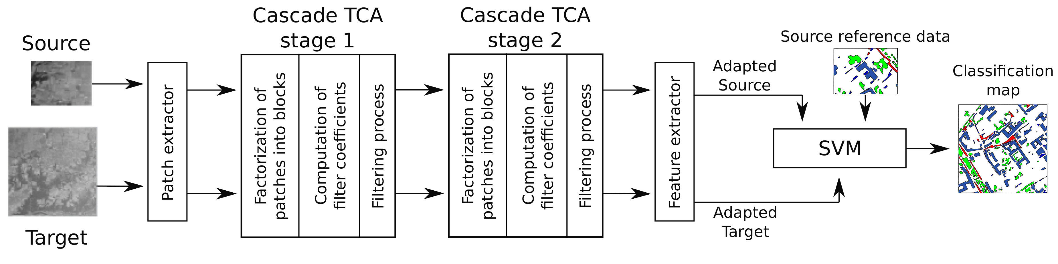
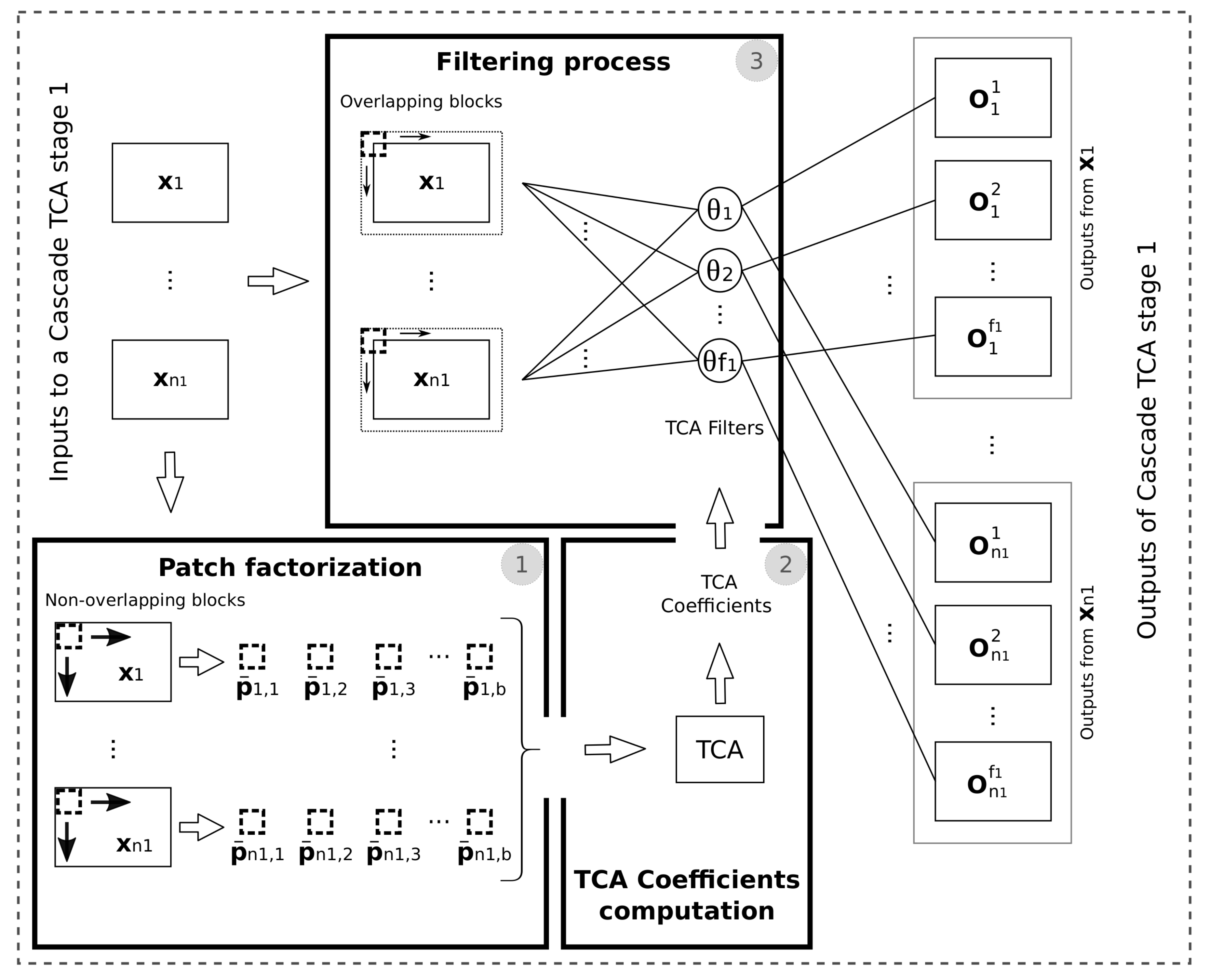
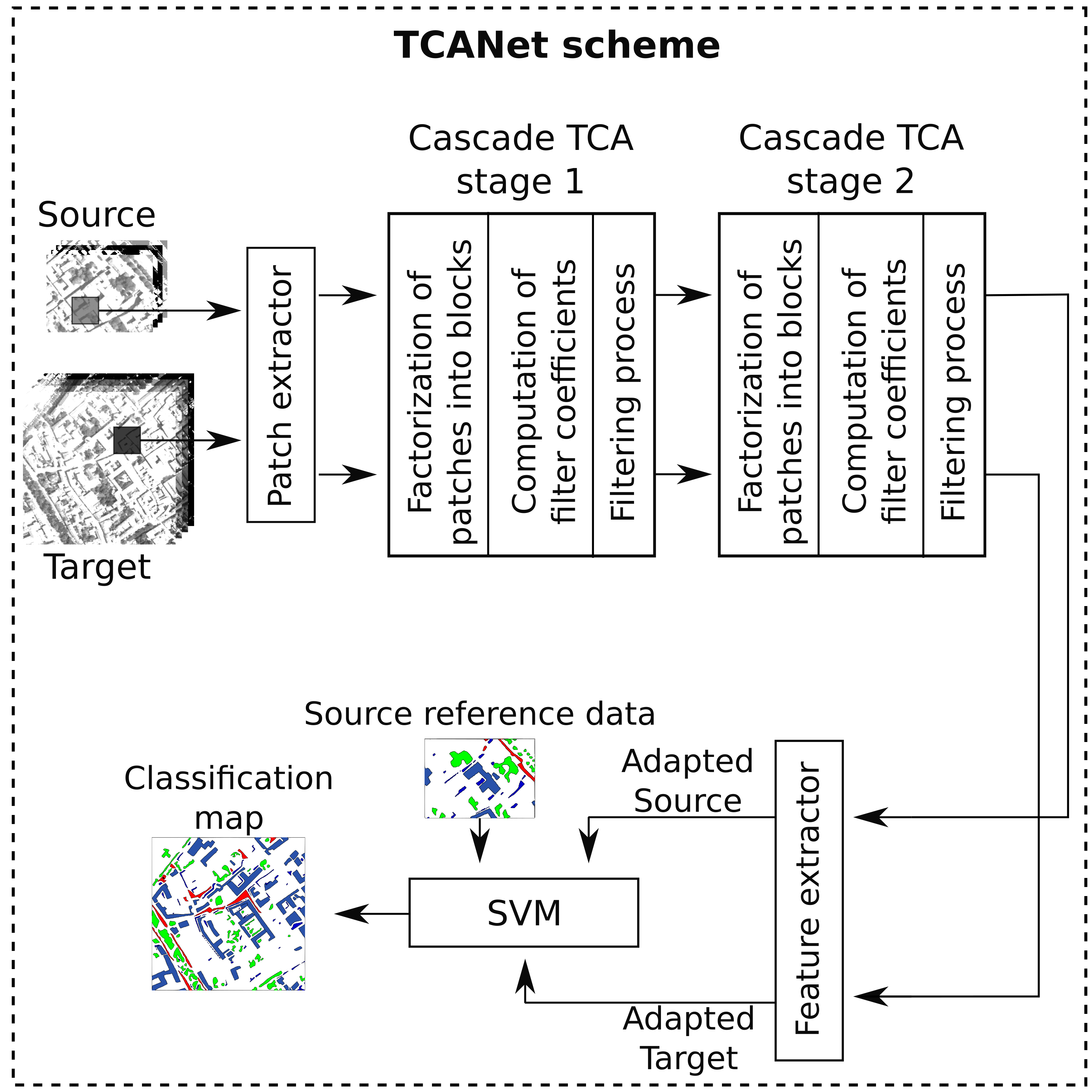
In this paper, a scheme for unsupervised DA applied for hyperspectral remote sensing classification, based on TCA and called TCA Network (TCANet) is proposed. It simulates the behaviour of a Convolutional Neural Network (CNN) with the particularity that the weights are fixed and computed based on TCA instead of being computed through a back-propagation algorithm, thus reducing the amount of time required for the computation of the weights. The scheme profits from the spatial information of the datasets by considering a patch around each pixel of the image as input. Then, TCA is applied to calculate the weights of the network. TCA tries to learn a transformation matrix across domains by minimizing the distribution distance measure. Since TCA is sensitive to normalization, to reduce the difference between source and target domains, a previous unsupervised domain shift minimization algorithm is conditionally applied. It aligns the second-order statistics of the source and target distributions. Finally, the output of the last layer is processed to extract the new modified features.

The paper is organized as follows: Section 2 presents some preliminary knowledge of DA and TCA and the data used in the experiments. Section 3 presents a detailed description of the proposed method. Section 4 presents the results obtained by the proposed scheme for the classification of hyperspectral images using DA. The discussion is performed in Section 5. Finally, Section 6 presents the conclusions.

2. Data and Techniques

In this section, the fundamentals required to understand the proposed scheme are presented. First, the DA problem in the terms studied in this paper is defined. Then, the TCA method for feature extraction is introduced as it is the base for the joint representation of the source and target images. Finally, the datasets used in the experiments are also detailed.

2.1. Domain Adaptation

As mentioned in Section 1, the proposed scheme makes an adaptation of the data distribution to reduce the data shift between the distributions of both source and target domains before the classification. To better identify the cases for which this solution can be used, we first describe the application context.

We consider a setting where all the labeled samples belong to the source domain and are used as training data. The test data is not labeled and belongs to the target domain. Thus, we can define the source domain as $D_S=\left\{({\mathbf{X}}_S,\mathbf{Y})\right\}=\{({{\mathbf{x}}_S}_1,y_1),\dots ,({{{\mathbf{x}}_S}_n}_s,{y_n}_s)\}$ where ${{\mathbf{x}}_S}_i\in {\mathcal{X}}_S$ is an input pixel and $y_i\in \mathcal{Y}$ denotes the corresponding output label, which is common to both source and target domains. Similarly, we define the target domain as $D_T=\left\{{\mathbf{X}}_T\right\}=\{\left({{\mathbf{x}}_T}_1\right),\dots ,\left({{{\mathbf{x}}_T}_n}_t\right)\}$ where ${{\mathbf{x}}_T}_i\in {\mathcal{X}}_T$ is the input data. Let $P\left({\mathbf{X}}_S\right)$ and $P\left({\mathbf{X}}_T\right)$ be the marginal probability distributions of ${\mathbf{X}}_S$ and ${\mathbf{X}}_T$, respectively.

In a typical domain adaptation context we assume that [33]:

• The input feature spaces are the same for both domains, ${\mathcal{X}}_S={\mathcal{X}}_T=\mathcal{X}$, and also the label space $\mathcal{Y}$.
• $P\left({\mathbf{X}}_S\right)\ne P\left({\mathbf{X}}_T\right)$, but $P\left(\mathbf{Y}\right|{\mathbf{X}}_S)=P\left(\mathbf{Y}\right|{\mathbf{X}}_T)$.

The first condition means that both domains have the same representation (in our case, the same number of bands in the images and the same number of classes in the reference data, for example). The second condition is equivalent to assume that both domains are correlated (the classes have distributions in the source and the target domains that can be related). Following this approach, in the scheme proposed in this work the only labeled samples that will be used belong to the source domain.

2.2. TCA for Feature Extraction

TCA [28] is a kernel-based feature extraction technique especially designed for DA. It tries to learn several transfer components across domains in a Reproducing Kernel Hilbert Space (RKHS), using Maximum Mean Discrepancy (MMD) [34] to minimize the distance between the distributions.

In contrast to other techniques, such as the Kullback–Leibler divergence, MMD is a non-parametric and computationally simpler kernel-based measure (involving the inner product between the difference in means of two groups’ features distributions [35]). The empirical estimate of the distance between two distributions, with data ${\mathbf{X}}_S$ (source) corresponding to the first distribution and data ${\mathbf{X}}_T$ (target) corresponding to the other one, such as being defined by MMD, is as follows:

$$\mathrm{dist}({\mathbf{X}}_S,{\mathbf{X}}_T)={∥\frac{1}{n_s}\sum _{i=1}^{n_s}\varphi \left({\mathbf{x}}_{S_i}\right)-\frac{1}{n_t}\sum _{i=1}^{n_t}\varphi \left({\mathbf{x}}_{T_i}\right)∥}_{\mathcal{H}}^2,$$

(1)

where $\mathcal{H}$ is a universal RKHS [36], and $\varphi :\mathcal{X}\to \mathcal{H}$ is a nonlinear mapping function that can be found minimizing the distance as defined by (1). Instead of this, [27] proposed to transform this problem into a kernel learning problem by using the kernel trick, (i.e., $K({\mathbf{x}}_i,{\mathbf{x}}_j)=\varphi {\left({\mathbf{x}}_i\right)}^{\prime }\varphi \left({\mathbf{x}}_j\right)$). Then, (1) can be rewritten as:

$$\mathrm{dist}({\mathbf{X}}_S,{\mathbf{X}}_T)=\mathrm{trace}\left(\mathbf{KL}\right),$$

(2)

where

$$\mathbf{K}=\left[\begin{array}{cc}{\mathbf{K}}_{S,S}& {\mathbf{K}}_{S,T}\\ {\mathbf{K}}_{T,S}& {\mathbf{K}}_{T,T}\end{array}\right]\in {\mathbb{R}}^{(n_s+n_t)\times (n_s+n_t)}$$

(3)

is a kernel matrix, ${\mathbf{K}}_{S,S}$ and ${\mathbf{K}}_{T,T}$ are the kernel matrices defined by $K\left(\right)$ on the source domain and target domain respectively, ${\mathbf{K}}_{S,T}$ and ${\mathbf{K}}_{T,S}$ are also kernel matrices defined by $K\left(\right)$ but on the cross-domain, and $\mathbf{L}=\left[L_{ij}\right]\ge 0$ with

$$\begin{array}{c}\hfill L_{ij}=\left\{\begin{array}{cc}\frac{1}{n_s^2}& \mathrm{if}{\mathbf{x}}_i,{\mathbf{x}}_j\in {\mathbf{X}}_S,\\ \frac{1}{n_t^2}& \mathrm{if}{\mathbf{x}}_i,{\mathbf{x}}_j\in {\mathbf{X}}_T,\\ -\frac{1}{n_s{n}_t}& \mathrm{otherwise}.\end{array}\right.\end{array}$$

(4)

The main objective of TCA is to find the nonlinear mapping function $\varphi$ based on kernel feature extraction. Ref. [28] proposes a unified kernel learning method using an explicit low-rank representation. Then, the kernel learning problem solved by TCA can be summarized as:

$$\begin{array}{cc}{\min }_w& \mathrm{trace}\left({\mathbf{W}}^{\mathrm{T}}\mathbf{W}\right)+\mu \mathrm{trace}\left({\mathbf{W}}^{\mathrm{T}}\mathbf{KLKW}\right)\\ \mathrm{s}.\mathrm{t}.& {\mathbf{W}}^{\mathrm{T}}\mathbf{KHKW}=\mathbf{I},\end{array}$$

(5)

where $\mu$ is a trade-off parameter, the second trace is the distance between mapped samples $\mathrm{dist}({\mathbf{X}}_S^{\prime },{\mathbf{X}}_T^{\prime })$ such that ${\mathbf{X}}_S^{\prime }=\left\{{\mathbf{x}}_{S_i}^{\prime }\right\}=\left\{\varphi \left({\mathbf{x}}_{S_i}\right)\right\}$, ${\mathbf{X}}_T^{\prime }=\left\{{\mathbf{x}}_{T_i}^{\prime }\right\}=\left\{\varphi \left({\mathbf{x}}_{T_i}\right)\right\}$, $\mathbf{I}$ is an identity matrix of size $m\times m$, and $\mathbf{H}$ is a centering matrix. The first trace in Equation (5) corresponds to a regularization term needed to control the complexity of the projection matrix $\mathbf{W}\in {\mathbb{R}}^{(n_s+n_t)\times m}$, $m\ll n_s+n_t$. This projection matrix is necessary to transform the corresponding feature vectors to the new m-dimensional space. The restriction ${\mathbf{W}}^{\mathrm{T}}\mathbf{KHKW}=\mathbf{I}$ is added to avoid the trivial solution ($\mathbf{W}=0$).

The optimization problem (5) can be reformulated as a trace maximization problem where the solution of the projection matrix $\mathbf{W}$ comes through the eigendecomposition of

$$\mathbf{E}={(\mathbf{I}+\mu \mathbf{KLK})}^{-1}\mathbf{KHK},$$

(6)

giving the m eigenvectors corresponding to the m principal eigenvalues of $\mathbf{E}$.

Once the fundamentals of TCA have been explained, we continue with the description of the datasets used in the experiments and the proposed TCANet scheme.

2.3. Data

The proposed scheme was evaluated over two remote sensing images acquired by two different sensors, ROSIS-03 and AVIRIS. The main specifications of these sensors are detailed in Table 1 [37,38,39,40,41,42].

Table 1. Main characteristics for both ROSIS-03 and AVIRIS sensors.

Characteristic	ROSIS-03	AVIRIS
Angular field of view (FOV)	16${}^{\circ }$	30${}^{\circ }$
Instantaneous field of view (IFOV)	0.56 mrad	0.95 mrad
Number of pixels per line	512	614
Scan principle	Pushbroom	Whiskbroom
Ground resolution	1 m–6 m	20 m
Radiometric resolution	14 bits	10 bits
Spectral range	430 nm–800 nm	400 nm–2450 nm
Spectral sampling	4 nm	9.6 nm–10.0 nm
Inflight calibration	0.2 nm	0.5 nm

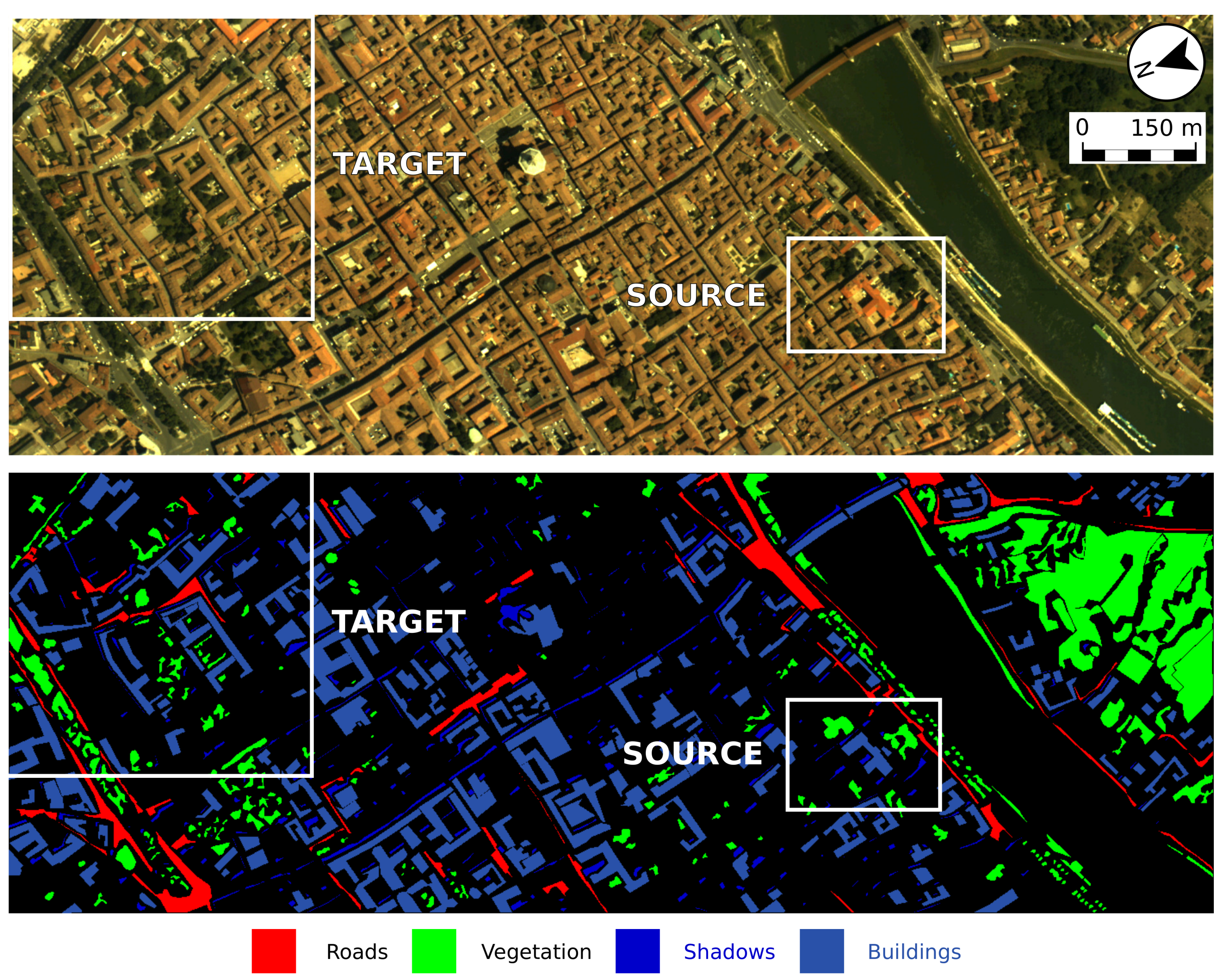
2.3.1. Pavia City Dataset

This image was acquired by the ROSIS-03 hyperspectral sensor covering the spectrum between 430 and 860 nm in 115 spectral bands over the city of Pavia. It has a spatial size of $512\times 1400$ pixels with a resolution of 1.3 m, and covers about 1 km². After removing noisy bands, the final spectral resolution of the image is 102 bands. Following the specifications of [21] two disjoint regions were used as source and target as can be seen in Figure 1 where the four different classes are specified. The source region has a size of $124\times 173$ pixels where its upper-left corner corresponds to the coordinates (907, 266) in the Pavia City image and its corresponding latitude and longitude are ${45}^{\circ }$10${}^{\prime }$54.95${}^{\prime }$${}^{\prime }$N and $9^{\circ }$09${}^{\prime }$21.09${}^{\prime }$${}^{\prime }$E, respectively. The target region has a spatial size of $350\times 350$ pixels where its upper-left corner corresponds to the coordinates (0, 0) in the original image and its corresponding latitude and longitude are ${45}^{\circ }$11${}^{\prime }$23.66${}^{\prime }$${}^{\prime }$N and ${09}^{\circ }$08${}^{\prime }$57.06${}^{\prime }$${}^{\prime }$E, respectively.

Figure 1. False color composite image, reference data and label meaning for the Pavia City dataset. Please note that the target and source domains are parts of the same image.

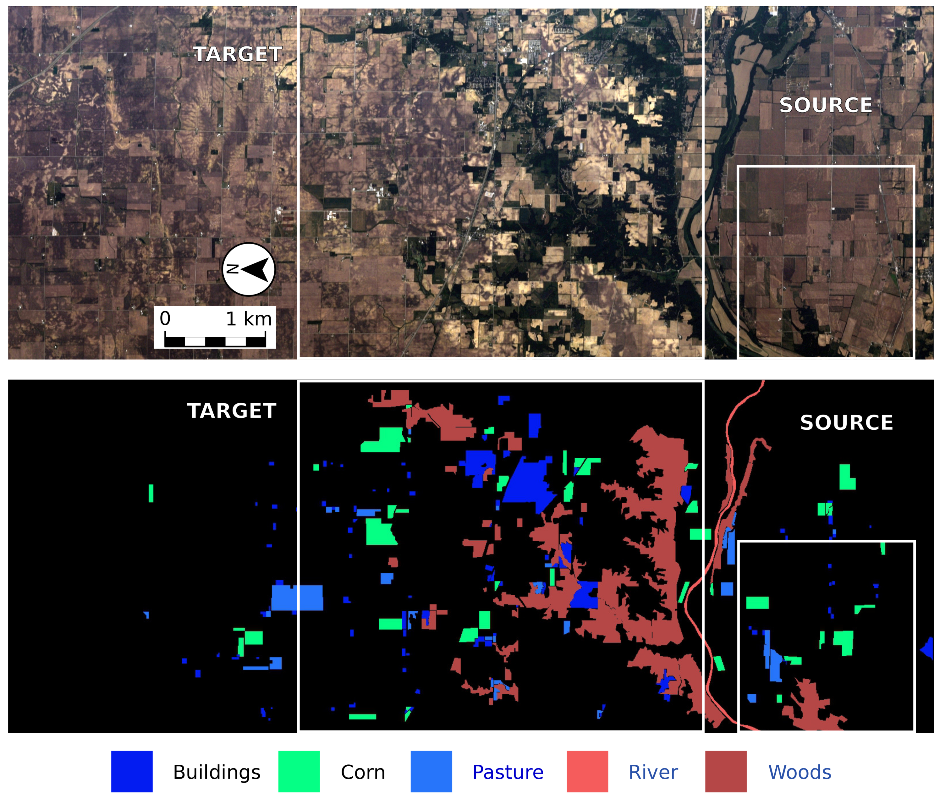
2.3.2. Indiana Dataset

This image was acquired by the AVIRIS hyperspectral sensor over the city of Indiana [43] on 12 June 1992. It has a spatial dimension of $2678\times 614$ pixels with a spatial resolution of 20 m and covers about 657 km². The spectral resolution is of 220 bands ranging 400–2500 nm. Two disjoint regions were used as source and target as shown in Figure 2 that was rotated 90 degrees to the left. On the one hand, the source region has a size of $301\times 329$ pixels where its upper-left corner corresponds to the coordinates (0, 2340) in the Indiana image and its corresponding latitude and longitude are ${40}^{\circ }$24${}^{\prime }$02.00${}^{\prime }$${}^{\prime }$N and ${87}^{\circ }$00${}^{\prime }$04.38${}^{\prime }$${}^{\prime }$O, respectively. On the other hand, the target region has a spatial resolution of $700\times 614$ pixels where its upper-left corner corresponds to the coordinates (0, 1576) in the original image and its corresponding latitude and longitude are ${40}^{\circ }$31${}^{\prime }$08.58${}^{\prime }$${}^{\prime }$N and ${86}^{\circ }$56${}^{\prime }$51.82${}^{\prime }$${}^{\prime }$O, respectively. The five classes shown in the figure were considered for this image in the experiments.

Figure 2. False color composite image, reference data and label meaning for the Indiana dataset.

3. TCANet: The Proposed Classification Scheme Based on DA

This section describes TCANet, the TCA-based classification scheme proposed in this paper. Its main goal is to achieve an adaptation of the domains of the source and target images in order to produce high classification accuracy. To achieve this goal, TCANet simulates the behaviour of a CNN. The network follows a similar philosophy as [24] in the sense that the convolutional filters are replaced by fixed filters. In the case of TCANet, the filters are computed using TCA, which is a method specifically designed for DA that minimizes the distance between the data distributions. Both source and target domains are used to compute the filters in order to find a new common representation.

Figure 3 shows a block diagram of the proposed scheme. After a first step where a set of patches are extracted from samples of the different images, two sequential cascade stages composed by a filtering process, a factorization of patches into blocks, and the computation of filter coefficients are applied to perform the DA task. In each cascade stage, TCA is applied to compute the transfer components needed to build the TCA filters that are used to perform the convolutional operation over all the previously extracted patches. The TCA filters are computed for each stage based on the output of the previous stage. Finally, a feature extraction step is carried out. This stage is responsible for producing the new features generated by the network. As a result a new representation of the samples is obtained. Once the images belong to the same domain, a classification process using Support Vector Machine (SVM) is performed. The different steps involved in the proposed scheme are explained along the next sections.

Figure 3. Block diagram of the classification scheme based on TCANet.

3.1. Patch Extraction

Suppose we are provided with two different remote sensing images $I_S$ and $I_T$, corresponding to the source and target domains respectively. Both images have the same number of bands (B) but not necessarily the same spatial size.

The first step in the process is to generate the input dataset containing samples selected from the source and target domains. Firstly, we select $n_S$ and $n_T$ random samples from $I_S$ and $I_T$, respectively. Then, in order to take advantage of spatial information, a patch of size $D\times D\times B$ around each sample is extracted being D the spatial width and height of the window and B the number of bands of each one of the images, that is ${\left\{{\mathbf{s}}_i\right\}}_{i=1}^{n_S},{\mathbf{s}}_i\in {\mathbb{R}}^{D\times D\times B}$ for the source, and ${\left\{{\mathbf{t}}_i\right\}}_{i=1}^{n_T},{\mathbf{t}}_i\in {\mathbb{R}}^{D\times D\times B}$ for the target. Then, each patch is reshaped from 3D ($D\times D\times B$) to 2D ($D^2\times B$). Therefore, the input for the next step is carried out by stacking $n_S$ patches from the source and $n_T$ patches from the target ${\left\{{\mathbf{x}}_i\right\}}_{i=1}^{n_1},{\mathbf{x}}_i\in {\mathbb{R}}^{D^2\times B},n_1=n_S+n_T$. A detailed example of the patch extraction process applied for one patch of the source and one patch of the target is shown in Figure 4 for 100-band source and target images ($B=100$).

Figure 4. Patch extraction example for a case of $D\times D\times B$ patches, being $D=3$ and $B=100$.

3.2. Cascade TCA

TCANet requires, as a standard CNN, different layers. In this paper two layers are considered. Each one of these layers is called a cascade TCA stage as it is shown in Figure 3. Each stage calculates the coefficients corresponding to the TCA filters from the patches provided by the previous stage. A general scheme of the cascade TCA stage 1 is shown in Figure 5. Three steps, each one marked with its corresponding execution position, can be identified: factorization of the patches into blocks, calculation of the filter coefficients, and filtering process. An identical structure is used for the cascade TCA stage 2 where the input data is the output of the cascade TCA stage 1. Any new stage would have the same structure.

Figure 5. Details of the cascade TCA stage 1.

3.2.1. Factorization of the Patches into Blocks

Unlike in [24] where overlapping blocks are extracted from each patch, TCANet extracts only non overlapping ones. This optimization highly reduces the amount of memory required and the computational cost. For each patch ${\mathbf{x}}_i$ that was obtained in the feature extraction process, b blocks of size $k_1\times k_2$ are extracted. Once all the blocks of ${\mathbf{x}}_i$ have been extracted, the block mean of this patch is subtracted from all of them obtaining ${\overline{\mathbf{P}}}_i=\left[{\overline{\mathbf{p}}}_{i,1},{\overline{\mathbf{p}}}_{i,2},\dots ,{\overline{\mathbf{p}}}_{i,b}\right]$, where ${\overline{\mathbf{p}}}_{i,j}$ is a mean-removed block. Figure 6 gives a graphical overview of the process. After applying the same process to all the ${\mathbf{x}}_i$ original patches we get

$$\mathbf{P}=\left[{\overline{\mathbf{P}}}_1,{\overline{\mathbf{P}}}_2,\dots ,{\overline{\mathbf{P}}}_{n_1}\right]\in {\mathbb{R}}^{k_1{k}_2\times n_{1}b}.$$

(7)

Figure 6. Detailed patch factorization scheme.

As soon as the blocks are obtained, the next step is to calculate the coefficients of the filters by using TCA.

3.2.2. Calculation of the Filter Coefficients

The filter coefficients are computed by applying the TCA algorithm presented in Section 2.2 to the extracted blocks. These are obtained by applying the next equation:

$${\mathbf{W}}_l={\mathrm{mat}}_{k_1,k_2}\left({\theta }_l\left(K({\mathbf{p}}_a,{\mathbf{p}}_b)\right)\right)\in {\mathbb{R}}^{k_1\times k_2},l=1,2,\dots ,f_1,$$

(8)

where ${\mathrm{mat}}_{k_1,k_2}\left(\mathbf{z}\right)$ is a function that maps $\mathbf{z}\in {\mathbb{R}}^{k_1{k}_2}$ to a matrix $\mathbf{W}$$\in {\mathbb{R}}^{k_1\times k_2}$, $K({\mathbf{p}}_a,{\mathbf{p}}_b)$ is a kernel function, ${\mathbf{p}}_a,{\mathbf{p}}_b\in \mathbf{P}$ are column vectors, ${\theta }_l(·)$ denotes the lth feature extracted using TCA, and $f_1$ is the number of filters of the first stage.

3.2.3. Filtering Process

Once the filter coefficients have been obtained, the next step is the filtering processing (convolution) of the ${\mathbf{x}}_i$ patches with the coefficients of each $f_1$ filter. The outputs for this first stage are:

$${\mathbf{O}}_i^l={\mathbf{x}}_i\ast {\mathbf{W}}_l^1,i=1,2,\dots ,n_1,l=1,2,\dots ,f_1,$$

(9)

where * denotes the 2D convolution. The total number of outputs generated in this first stage of the cascade TCA is $n_2=n_1\times f_1$.

As soon as the output of the cascade TCA stage 1 is obtained, the same steps (factorization of the patches into blocks, calculation of the filter coefficients and filtering process) are performed to complete the cascade TCA stage 2. As input for this stage, the output of the previous cascade TCA stage is used.

3.3. Feature Extraction

Once the two cascade TCA stages are processed, the next stage is the extraction of the new features for the input samples. This stage consists of the steps explained below. An example of this process is shown in Figure 7 for an input patch with $D=3$ and $B=1$, where D is the spatial width and height of the window and B is the number of bands of the images. Please note that the patch size used in the real experiments is higher, as it will be described in the results section.

Figure 7. Example of feature extraction scheme considering input patches of $3\times 3$ pixels.

The number of outputs for each initial input patch ${\mathbf{x}}_i$ produced by the last cascade TCA stage is $f_1\times f_2$ (first column in Figure 7). Once all the outputs of the last stage have been computed, they are binarized using the Heaviside function $\mathcal{H}(·)$. This function returns 0 when the value is less or equal than 0 and 1 otherwise. After that, the outputs containing only binary values are grouped into sets of $f_2$ elements. Finally, these elements are reduced by adding all the values component by component (denoted as addition of matrices in the figure), considering all the $n_t$ patches in the images the result of the reduction will be:

$${\mathcal{T}}_c=\sum _{v=1}^{f_2}\left(\mathcal{H}\left({\mathbf{O}}_c^v\right)\right),c=1,2,\dots ,n_t\times f_1.$$

(10)

The final feature for each initial input patch ${\mathbf{x}}_i$ (last column in Figure 7) is defined as:

$${\mathbf{f}}_i={[\mathcal{S}\left({\mathcal{T}}_{(((i-1)\times f_1)+1)}\right),\dots ,\mathcal{S}\left({\mathcal{T}}_{(i\times f_1)}\right)]}^T,$$

(11)

where $\mathcal{S}(·)$ is a binary function that returns zero if the input value is less than the smallest integer that is greater than or equal to $f_2/2$ and one otherwise. Thus, the size of each ${\mathbf{f}}_i$ is $D^2\times B\times f_1$.

3.4. Conditional Correlation Alignment (CCA)

Since TCA is sensitive to normalization, [44] proposed a variant called TCA+ which automatically selects a suitable normalization for the source and target data before applying TCA. This normalization is based on the means and standard deviations of the overall Euclidean distance of all pairs of instances of the datasets. In our case, we propose a simple method, see Figure 8, for unsupervised domain adaptation similar to the technique called CORrelation ALignment (CORAL) [14]. Based on the covariance alignment of both source and target distributions, the domain shift is minimized by applying a linear transformation. We propose a conditional application of the correlation alignment called CCA over the original datasets. It applies correlation alignment only if the distance between the two distributions of the source and target domains ($D_S$ and $D_T$) decreases after applying the correlation alignment. The metric used is the mean Mahalanobis distance (MD) calculated between all pixel pairs.

Figure 8. Conditional Correlation Alignment (CCA) scheme.

4. Results

This section presents the experimental results obtained by applying TCANet for DA over the two datasets described in Section 2.3. Each dataset consists of two images, source and target. As the task performed is classification, the results are shown in terms of classification accuracy.

The proposed scheme was evaluated on a PC with a quad-core Intel i5-6600 at 3.3GHz and 32 GB of RAM. The codes were implemented using MATLAB version 2015B, TensorFlow 1.3.0 and Pytorch 0.4.0. Regarding the GPU implementation, TensorFlow codes run on a Pascal NVIDIA GeForce GTX 1070 with 15 Streaming Multiprocessors (SMs) and 128 CUDA cores each. The CUDA version used is 8.0.61.

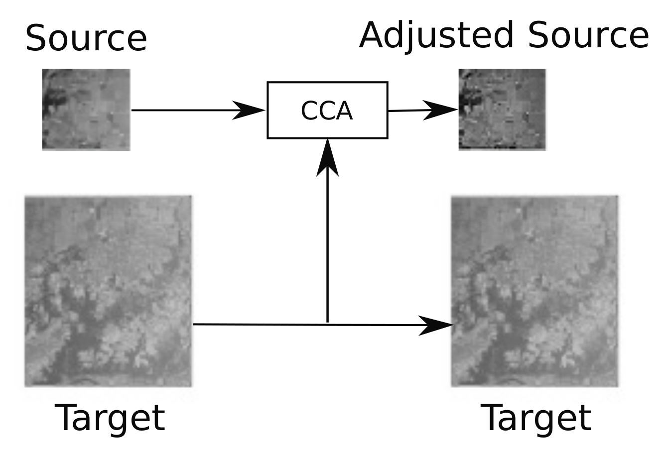
When applying the proposed TCANet, a first preprocessing step consisting of a conditional correlation alignment is applied, as explained in Section 3.4. To decide whether CCA is applied, the Mahalanobis distance between the input image and the target image, after and before the correlation alignment, are calculated. Table 2 shows the results. ${\mathrm{MD}}^{\prime }$ denotes the distance calculated for the adjusted source data and $\mathrm{MD}$ the distance for the original source data as defined in Algorithm 1. In the case of the Indiana dataset, it is clear that applying correlation alignment increases the distance value, so in this case this correlation alignment is not applied. The situation is the opposite for the other dataset.

Algorithm 1 CCA algorithm

Input: Source Data ${\mathbf{D}}_S$, Target Data ${\mathbf{D}}_T$ Output: Adjusted Source Data ${\mathbf{D}}_S^{\prime }$ ${\mathbf{C}}_S=\mathrm{cov}\left({\mathbf{D}}_S\right)+\mathbf{I}$ ${\mathbf{C}}_T=\mathrm{cov}\left({\mathbf{D}}_T\right)+\mathbf{I}$ ${\mathbf{E}}_S={\mathbf{D}}_S{\mathbf{C}}_S^{\frac{-1}{2}}$ ${\mathbf{D}}_S^{\prime }={\mathbf{E}}_S{\mathbf{C}}_T^{\frac{1}{2}}$ if$\mathrm{MD}({\mathbf{D}}_S,{\mathbf{D}}_T)<=\mathrm{MD}({\mathbf{D}}_S^{\prime },{\mathbf{D}}_T)$then ${\mathbf{D}}_S^{\prime }={\mathbf{D}}_S$ end if

Table 2. Mahalanobis distance between samples from source and target.

Datasets	Distance
	${\mathrm{MD}}^{\prime }$	$\mathrm{MD}$
Pavia City	136.58	139.88
Indiana	22,348.85	364.22

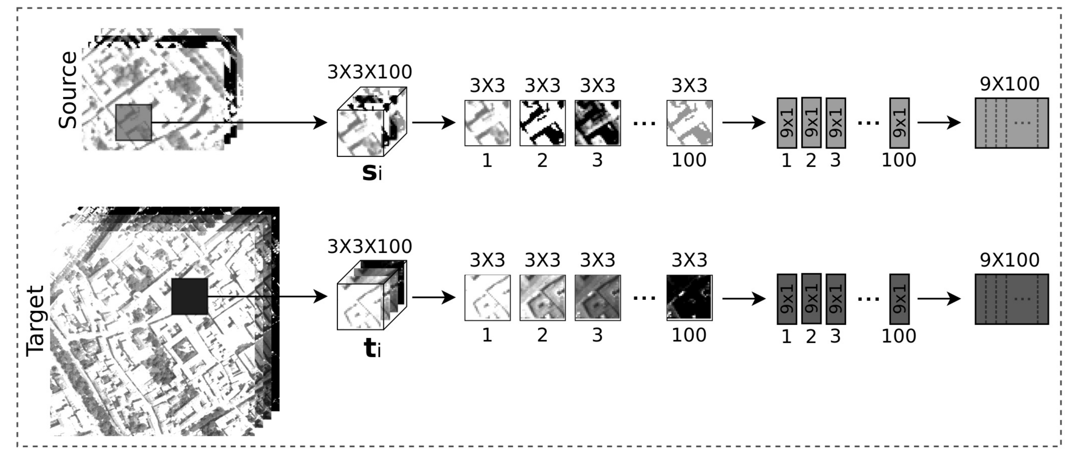
For the proposed TCANet scheme two cascade TCA stages are used. The input patches are of a spatial size of $3\times 3$ and 100 bands in the case of Pavia, and $3\times 3$ and 220 bands in the case of Indiana. As a result a patch size of $3\times 3\times 100$ and $3\times 3\times 220$, for Pavia and Indiana, respectively, are produced. The block sizes are $9\times 50$ for Pavia and $9\times 55$ for Indiana. The filter sizes for the $f_1$ and $f_2$ filters are 2 and 16, respectively. Regarding the feature extraction stage, each input patch of size $D\times D\times B$ is represented by a final feature vector of size $D\times D\times B\times f_1$, being $f_1$ the number of filters in the first cascade TCA stage. As a result, for the Pavia dataset the size of the output features is 1800, while the size is 3960 for Indiana.

The evaluation of the TCANet proposed scheme is carried out by using a final SVM classification stage. As usual in remote sensing [45], the classification accuracy results are presented in terms of overall accuracy (OA), which is the percentage of correctly classified pixels compared to the reference data information available, average accuracy (AA), which is the mean of the percentage of correctly classified pixels for each class, and kappa coefficient (K) which is the percentage of agreement (correctly classified pixels) corrected by the number of agreements that would be expected purely by chance [46,47]. Furthermore, for the proposed scheme, a F1-score [48] values corresponding to the macro-average F1-score values computed as the arithmetic mean of the per-class F1-score have been included. The results are the average of 10 independent executions.

To analyse the performance of the different schemes and compare to the state of the art, similar settings to [21] were used. The number of available samples from both source and target domains for the two images (Pavia City and Indiana) are displayed in Table 3 and Table 4. A maximum number of 200 labeled samples per class were selected for training from the source image. In those classes in which the number of samples were less than 200, all available samples were selected. Similar to [21], only 50% of the target samples were used for test.

Table 3. Samples available in the Pavia City dataset.

Classes	Source		Target
	Samples	%	Samples	%
Roads	326	7.96	2549	9.07
Vegetation	1793	43.75	6406	22.80
Shadows	514	12.54	1638	5.83
Buildings	1465	35.75	17,501	62.29
Total	4098		28,094

Table 4. Samples available in the Indiana dataset.

Classes	Source		Target
	Samples	%	Samples	%
Buildings	432	4.33	15,003	17.64
Corn	3062	30.69	11,116	13.07
Pasture	1742	17.47	4154	4.88
River	197	1.97	540	0.63
Woods	4543	45.54	54,230	63.77
Total	9976		85,043

The DA method proposed in this paper as well as the other methods presented for comparison consist of two steps. The first one builds a mapping function $\mathsf{\Theta }$ based on representation learning algorithms where the original features are transformed into others that can increase the separability of the different classes. The second step creates a model based on SVM using the transformed training set to train the model and performing the final classification over the transformed test set.

Table 5 shows the origin of the samples used for the representation learning and the classification steps for all the methods analyzed. Subscripts S and T denote the source and target domains, respectively. In all the methods where samples belonging the target set were used to build the mapping function these samples were not used in the classification step. The only methods for which no representation learning is applied are the SVM-Src and the SVM-Tgt methods. Thus, the inputs for the classifier in these cases are the original features.

Table 5. Sample selection.

Method	Rep. Learning Samples	Classification
		Train Set	Test Set
SVM-Src	-	${\mathcal{X}}_S$	${\mathcal{X}}_T$
SVM-Tgt	-	${\mathcal{X}}_T$	${\mathcal{X}}_T$
1DOM	${\mathcal{X}}_S$	$\mathsf{\Theta }\left({\mathcal{X}}_S\right)$	$\mathsf{\Theta }\left({\mathcal{X}}_T\right)$
2DOM	${\mathcal{X}}_S\cup {\mathcal{X}}_T$	$\mathsf{\Theta }\left({\mathcal{X}}_S\right)$	$\mathsf{\Theta }\left({\mathcal{X}}_T\right)$
DANN	${\mathcal{X}}_S\cup {\mathcal{X}}_T$	$\mathsf{\Theta }\left({\mathcal{X}}_S\right)$	$\mathsf{\Theta }\left({\mathcal{X}}_T\right)$
TCANet	${\mathcal{X}}_S\cup {\mathcal{X}}_T$	$\mathsf{\Theta }\left({\mathcal{X}}_S\right)$	$\mathsf{\Theta }\left({\mathcal{X}}_T\right)$

The methods where only samples from the source domain are used to obtain the mapping function are labeled as “1DOM”. The methods that use some unlabeled samples from the target domain, in addition to the samples of the source domain to generate the mapping function are labeled as “2DOM”. By definition, both DANN and TCANet methods fit a “2DOM” setting since both of them use a small set of unlabeled samples from the target domain. For the classification step, a SVM with a radial basis function (RBF) kernel is used. Five-fold cross-validation [49] to find the values of parameters C and $\gamma$ that optimise the OA value obtained by SVM was used. For C the range of values used goes from −1 to 15 and for $\gamma$ the range goes from −10 to 10. In both cases the step size was 1.

Table 6 and Table 7 show the results of the different methods applied over the Pavia City and Indiana datasets, respectively. SVM-Src uses samples from the source for training and samples from the target for test. In the case of SVM-Tgt, non-overlapping sets of samples from the target are used for both training and test. The number of samples from the target, used in the training step, for the SVM-Tgt method is 200 per class. For those classes for which the number of samples is less than 200, all the samples were selected.

Table 6. Results for the Pavia City dataset.

Method	OA (%)	AA (%)	K (%)	F1-Score (%)
SVM-Src [21]	91.80	85.70	84.50	-
SVM-Tgt [21]	92.00	95.20	86.00	-
PCA-1DOM [21]	87.60	76.20	77.00	-
PCA-2DOM [21]	90.50	82.40	82.10	-
DAE-1DOM [21]	92.40	93.20	86.80	-
DAE-2DOM [21]	92.10	93.70	86.30	-
DANN [21]	92.60	85.40	86.80	-
TCANet	93.82	92.01	88.77	89.62

Table 7. Results for the Indiana dataset.

Method	OA(%)	AA(%)	K(%)	F1-Score(%)
SVM-Src	50.84	56.42	28.54	-
SVM-Tgt	79.69	84.54	64.87	-
PCA-1DOM	55.86	63.26	34.02	-
PCA-2DOM	53.68	58.80	31.21	-
DAE-1DOM	53.95	59.90	32.21	-
DAE-2DOM	78.99	83.97	63.88	-
DANN	50.30	63.50	30.36	-
TCANet	78.22	71.15	58.80	68.97

The methods denoted as PCA-1DOM and PCA-2DOM, extract features from the inputs by computing PCA previously to the classification by SVM. The number of principal components selected for the experiments was obtained as the value in the range going from 2 to the number of bands of each image with a step size 2, that produced the best OA value.

For the DAE methods, an simple hidden layer of 200 and 400 neurons for the Pavia City and Indiana datasets, respectively, was used. Regarding all other parameters, the two images used the same values, which are $learning\_rate=0.1$, $momentum=0.00005$ and a Gaussian noise with $standard\_deviation=0.1$. The DANN method is the only one that does not need the SVM classifier. The method itself integrates both the representation and the classification steps. For the representation step, a network with three hidden layers of size 50 was used for the two images. A similar configuration was applied to the classification step. The other parameters used for this method are $number\_of\_epochs=250$, $batch\_size=32$, $momentum=0.9$ and $learning\_rate=0.001$.

5. Discussion

The results in Table 6 show that our method outperforms the other alternatives for the Pavia dataset while in Table 7 the proposed method is among the best results for Indiana. In this case the results are slightly below those obtained by the DAE-2DOM method, but with a better standard deviation, 1.01 for our method compared to 1.50 obtained by DAE-2DOM.

The use of networks such as TCANet, with a CNN-like structure but simpler filter calculation, allows reducing the computational cost of training the network by replacing the repetitive training process to compute the weights of the network by methods that use fixed weights computed directly. Inputs coming from the source and the target domains are used for computing the fixed filters, so the filter learning in TCANet does not involve regularized parameters and does not require numerical optimization solvers. In summary, the method includes only a cascaded linear map, followed by a nonlinear output stage. The proposal offers simplicity and effectiveness. As a possible limitation we could mention the high memory requirements of the TCA computation. The reason is that it requires the computation of several matrix multiplications with a size of the matrix involved in the operations depending on the number of samples selected for training from both the source and the target. To reduce the computational cost, other TCA algorithms could be tried.

As future work, from the implementation point of view we will focus on optimizing the computational cost of TCANet in order to make a fair comparison to the cost of a standard CNN. The present version of TCANet includes non-optimized functions, as for example, those computed using MATLAB. These functions should be rewritten in CUDA, for example, thus exploiting the computational capabilities of Nvidia GPUs and allow a fair comparison with the CNN implementations usually used as reference for computational cost and execution time measurement. From the DA perspective, the proposed scheme based on the computation of fixed filters could be adapted to use other TL algorithms to obtain the filters. In particular, other methods derived from TCA that offer better results for some datasets could be applied. A detailed study considering a tradeoff between computational cost and accuracy in the TL process is required for the selection of the best network structure.

6. Conclusions

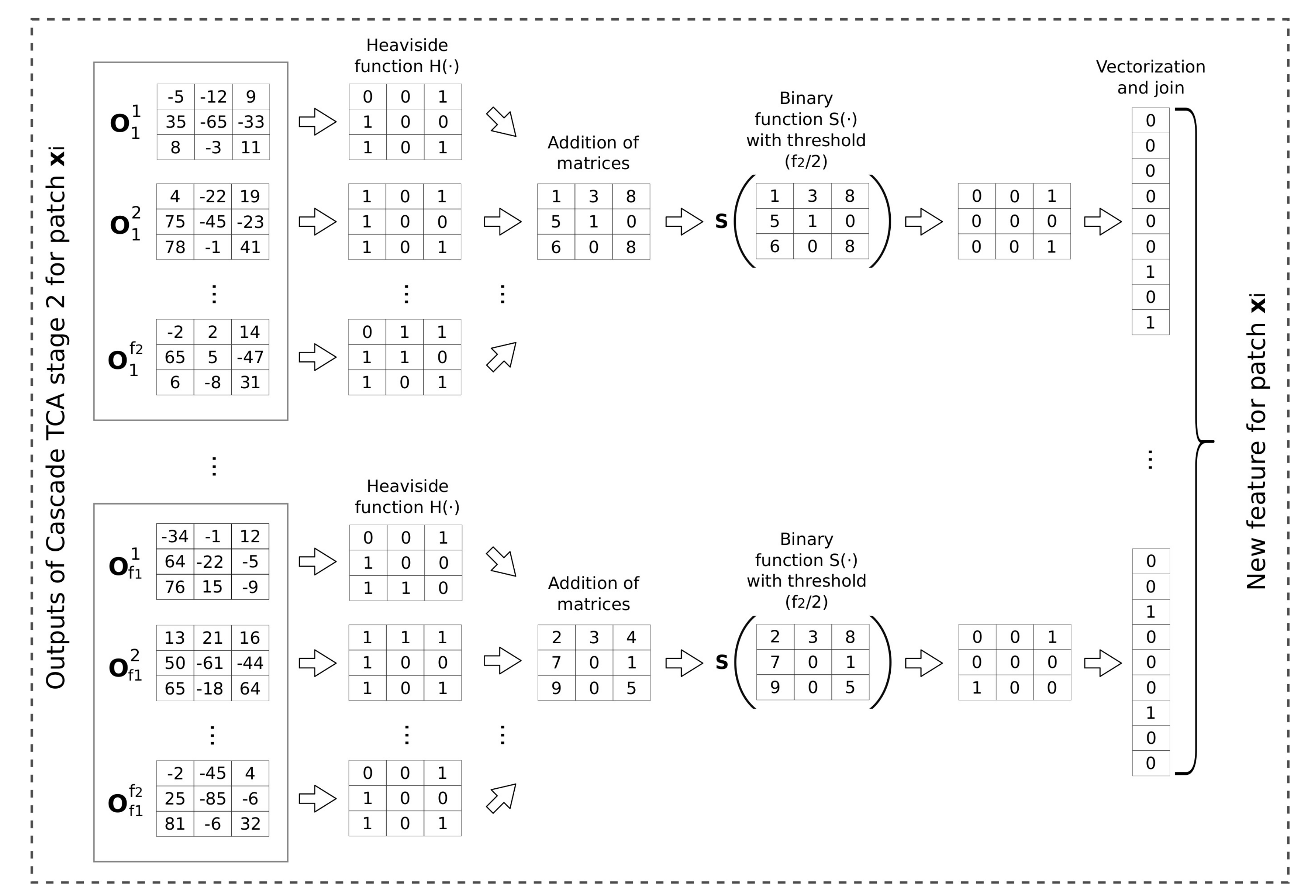
In this paper, a network scheme for Domain Adaptation (DA) of hyperspectral images based on Transform Component Analysis (TCA) is proposed. The scheme, called TCANet, has a structure similar to a Convolutional Neural Network (CNN), but differs from the latter in that coefficients of the convolutional filters are computed using the TCA algorithm. That is, the filter coefficients are obtained directly on the input data, from both the source and the target domains, requiring no backpropagation learning. TCA shares some characteristics with Principal Component Analysis (PCA), but while PCA is a generic method of dimensionality reduction, TCA is a method especially designed for DA that minimize the difference in distributions of data in different domains. Additionally to the convolutional filter stages, TCANet includes a stage of patch extraction, a conditional correlation alignment using the second-order statistic to reduce the domain shift between the source and the target domains, and a final stage based on Heaviside functions to perform feature extraction. The scheme takes into account both spatial and spectral information.

In summary, the scheme simulates the behaviour of a CNN specifically adapted to DA, requiring no backpropagation algorithm, and therefore reducing the computational cost. The classification accuracy obtained by SVM using the proposed network for DA was evaluated using two standard datasets (Pavia City and Indiana) obtaining competitive results with respect to other deep learning methods. On the other hand, the network scheme is quite general in the sense that TCA could be replaced by other DA algorithms that perform representation learning or feature extraction.