A Simultaneous Imaging Scheme of Stationary Clutter and Moving Targets for Maritime Scenarios with the First Chinese Dual-Channel Spaceborne SAR Sensor

Abstract

The technique of azimuth multichannel synthetic aperture radar (SAR) system has become a potential solution to the irreconcilable conflict between high-resolution and wide-swath (HRWS) confronted with in a traditional SAR system. Unambiguous imaging, especially for a scene with moving targets, is one of the crucial research topics in the HRWS SAR system. This paper proposes a simultaneous imaging scheme of moving targets and stationary clutter for maritime scenarios. First, the moving target echoes are extracted from the stationary clutter. After that, two methods working in completely different principles are used to estimate the radial velocity of each moving target, and the estimated result is used for phase compensation. After that, the moving target echoes are added back to the stationary scene echo and sent to the reconstruction filter. Lastly, the reconstructed echo can be processed by the classical Chirp Scaling (CS) algorithm. Experiments are carried out using the Chinese GaoFen-3 dual-channel data. The estimated velocities of the moving targets are verified by automatic identification service (AIS) information, and the imaging results show that the false targets are effectively suppressed and the moving targets also return to their correct positions along the azimuth.

1. Introduction

Synthetic aperture radar (SAR) is a powerful tool in many fields such as disaster management, sea traffic observation, and environmental monitoring. However, traditional SAR systems cannot meet the increasing requirements of the high-resolution and wide-swath (HRWS) at the same time, since they have different requirements for the spatial sampling rate in azimuth, i.e., pulse repetition frequency (PRF). High azimuth resolution requires a high PRF, while a low PRF is needed to unambiguously image a wide swath [1]. The azimuth multichannel SAR system, which employs multiple receiving apertures to gather information along the synthetic aperture plays an essential role in HRWS imaging since it can overcome the inherent limitations [2]. The radar PRF in each channel is less than the single-channel system in order to avoid an ambiguous range, and the echoes of multiple channels are processed together to obtain high azimuth resolution.

GaoFen-3 (GF-3) is a Chinese spacecraft carrying a C-band SAR (5.4 GHz) launched in August 2016 [3,4]. GF-3 is also the first Chinese multi-channel SAR sensor working in the dual receiving channel (DRC) mode (or named ultra-fine stripmap (UFS) mode), which is one of the 12 observing modes. The main challenge the DRC mode faces is the Doppler spectrum alias caused by many factors, which leads to the existence of false targets.

Channel imbalances, non-uniform sampling, and the presence of moving targets are the main causes of the Doppler spectrum aliasing. For the static scenes, unambiguous imaging can be achieved by estimating and compensating the amplitude and phase errors between different channels [5,6,7] and by the reconstruction algorithm, which solves the non-uniform sampling problem [8]. The first spaceborne demonstration experiment using the TerraSAR-X dual receiving antenna mode is elaborated in Reference [9], and the processing algorithms for the GF-3 dual-channel mode imaging are described in References [5] and [10]. Nevertheless, the false targets still exist if there are moving targets and they are treated as stationary ones [10,11,12]. False targets (or named ghost targets) of the moving target must be suppressed, especially for the maritime scenarios. Since there are lots of moving vessels in the maritime scenarios, usually the scattering coefficients of the vessels are much higher than that of the sea clutter. Even if the power of the false targets is 20dB lower than their corresponding real targets, the existence of false targets will still increase the false alarm probability of ship detection and affect the interpretation of SAR images [13].

A classical multi-channel ground moving target indication (GMTI) and clutter suppression techniques, such as displaced phase center antenna (DPCA) [14,15,16], along-track interferometry (ATI) [17,18], and space-time adaptive processing (STAP) [19,20], improve moving target detection performance significantly. However, their demand on the radar PRF in each channel is higher than the Doppler bandwidth. Therefore, these methods are not suitable for the HRWS system. To solve this problem, Baumgartner at al. proposed the HRWS-DPCA algorithm in Reference [21]. For the application of the algorithm, the conventional HRWS SAR imaging system needs to be extended by some additional receiving channels or transmitting channels, which makes the system complicated. In addition, a robust clutter suppression approach is proposed for HRWS SAR in Reference [22]. A group of filters is constructed to null the clutter directions and preserve the energy of the signals at the potential moving targets direction in the range compression and azimuth chirp Fourier transform frequency (RC-CFT) domain. However, for the maritime scenarios, since moving targets are sparse with strong signals embedded in a rather weak clutter environment, the clutter suppression and moving target indication is not the key issue. A more efficient and effective approach should be adopted.

There has been more research on the subsequent velocity estimation, particularly radial velocity estimation of the moving target. Some methods work well for the conventional multichannel SAR system when the signals of each channel are over-sampled in the image domain [23,24]. For the HRWS SAR system, methods carried out in the signal domain to estimate velocity is proposed in References [25,26]. The method described in Reference [25] estimates the velocity by estimating the direction-of-arrival (DOA) of the signal. A velocity estimation algorithm proposed in Reference [26] is based on the analysis of signal subspace and noise subspace, but the method suffers from the limitation of at least one redundant channel, which means the number of RX antennas should be greater than the Doppler ambiguity number. In addition, a novel algorithm for velocity estimation conducted in the echo domain is proposed in Reference [10], which applies the maximum likelihood (ML) method to estimate the cone angle as well as the radial velocity.

Conventional HRWS SAR imaging algorithms were developed for unambiguous Doppler spectrum reconstruction and azimuth ambiguity cancellation of stationary, but not moving target signals. However, the moving target imaging algorithm for the HRWS SAR systems described in the literature, such as References [11,22], only obtains a well-focused moving target image. Particularly, there are currently few studies to provide a simultaneous imaging scheme of stationary clutter and moving targets. For some special applications, users might prefer the wide-area and high-resolution image with both unambiguous stationary scenes and well-focused moving targets in their right position.

In this paper, a simultaneous imaging scheme of stationary clutter and moving targets for maritime scenarios is proposed. Given that the moving targets with strong energy are embedded in a rather weak clutter environment, their echoes are detected and extracted in range time-azimuth dechirp frequency domain efficiently and effectively. In order to make the scheme suitable for any Signal-to-Clutter Ratio (SCR) situation, two methods carried out in the signal domain, i.e., time domain correlation (TDC) method and maximum likelihood (ML)-based algorithm, are applied to estimate the radial velocity of each of the moving targets. To verify the correctness of the estimated radial velocity, it is converted to the ground velocity, i.e., cross-track velocity component on the ground. The target’s along-track velocity component that causes the image defocusing is obtained by the autofocus algorithm [27,28]. The ship’s velocity calculated by combining the cross-track component and along-track component is confirmed by comparing the velocity in the automatic identification service (AIS) [29] sensor data. The rest of the paper is organized as follows. In Section 2, the imaging geometry model of the GF-3 DRC mode is described and the signal echo model of the moving target is analyzed. Several techniques of the imaging process including extraction of moving target echoes, the radial velocity estimation, and the compensated phase introduced by radial velocity are explained in Section 3. Experimental results based on the simulation and GF-3 real data are presented in Section 4, which is followed by some discussion of the experiments in Section 5. Section 6 draws the conclusions.

2. Geometry Model and Signal Model

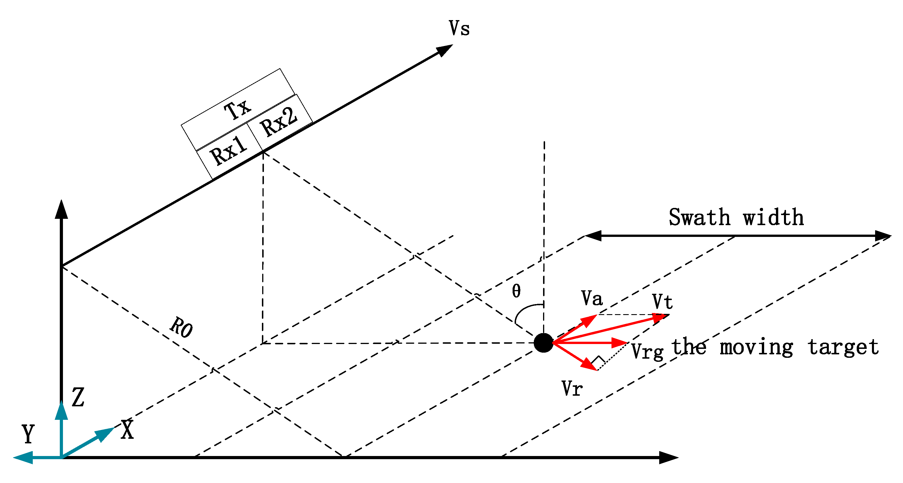
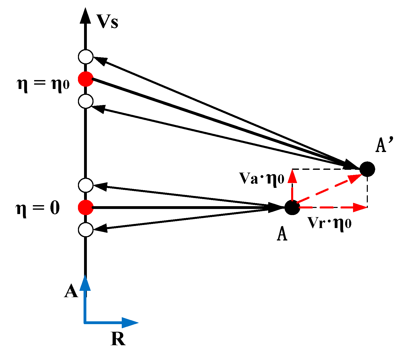
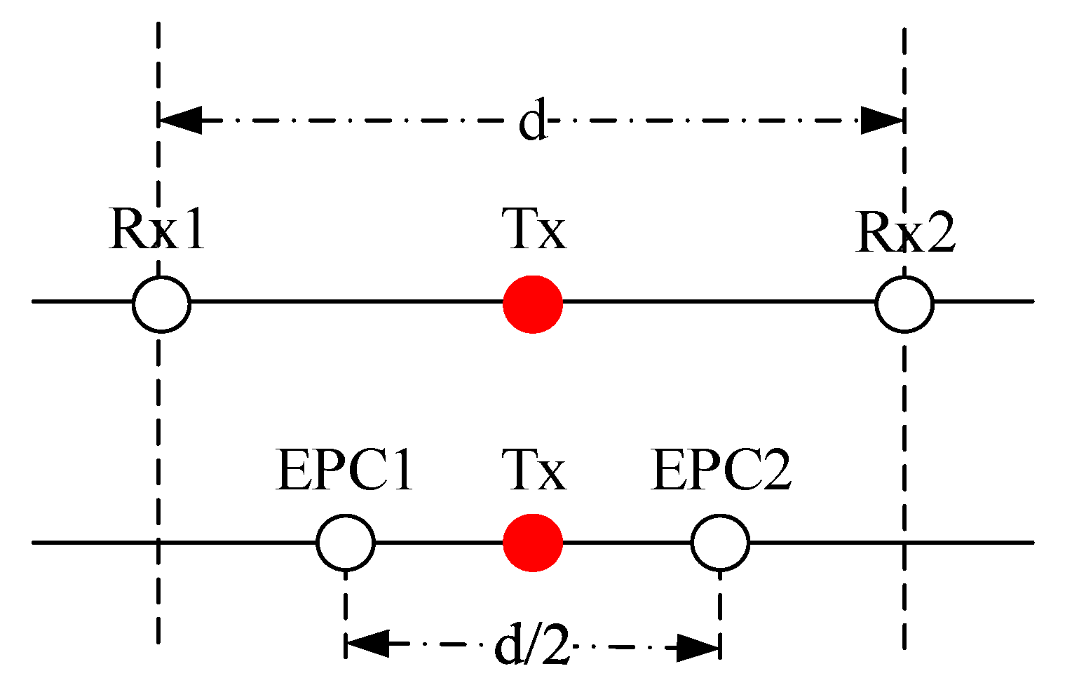
2.1. Imaging Geometry Model of Dual Receive Channel Mode

Figure 1 illustrates the imaging geometry for the side-looking mode of the GF-3 DRC mode, where the $\mathrm{x}$-axis is in the direction of the platform velocity $V_s$, the $\mathrm{z}$-axis is always from the center of the earth, and the $\mathrm{y}$-axis point to the left, which completes the orthogonal right-handed frame. There is a moving target at the center of the scene where the incidence angle is $\mathsf{\theta }$, and its velocity is $V_t,$ which is along the earth surface. $V_t$ can be decomposed into along-track velocity $V_a$ and the cross-track velocity $V_{rg}$, and then the radial velocity $V_r$ is the projection of the cross-track velocity $V_{rg}$ on the slant range direction. The relationship between $V_r$ and $V_{rg}$ can be written below.

$$V_{rg}=\frac{V_r}{\sin \left(\theta \right)}.$$

(1)

For the convenience of expression, the moving target is modeled as an ideal point target. The entire antenna is employed to transmit the chirp signal and is divided into two sub-apertures to receive echoes. $\mathrm{Tx}$ represents the transmit phase center, and $\mathrm{Rx}1$ and $\mathrm{Rx}2$ represent the phase centers of two actual receiving antennas. By compensating a constant phase with respect to the reference channel, the received data can be converted into the equivalent self-transmitting and self-receiving data corresponding to the effective phase center (EPC) [2]. Figure 2 shows the relationship between actual receiving channels and effective receiving channels. The distance between adjacent actual phase centers is $d$, while that between adjacent EPCs is $d/2$.

The geometry between the platform and the moving target at different azimuth time in the slant-range plane is shown in Figure 3. The red solid circle represents the phase center of the transmitting antenna, while the white circle represents the EPCs. During the radar observation time duration ${\eta }_0$, the target moves from position $\mathrm{A}$ to ${\mathrm{A}}^{\prime }$.

2.2. Signal Model

The symbols of the parameters used in this paper are listed as follows.

$m$	Index of receive channels, $m=1,2$,
$\mathsf{\tau },\mathsf{\eta }$	Range time and azimuth time, respectively,
$R_0$	The closest slant range of the moving target,
$V_s$	Platform velocity,
$V_r,V_a$	Radial velocity and along-track velocity, respectively,
$x_{m\_epc}$	Azimuth position of $m$-th EPC,
$d$	Distance between adjacent actual receive channels,
$T_p,K_r$	Pulse width and chirp rate of the transmitted signal, respectively,
$T_s$	Synthetic aperture time,
PRF	Pulse repetition frequency for each channel,
$\lambda$	The wavelength of the radar signal,
$c$	Light speed.

According to the geometry of the GF-3 DRC mode for the side-looking mode, the instantaneous slant range between the $m$-th EPC and the moving target at the center of the scene can be expressed as:

$$R_m\left(\eta \right)= \sqrt{{\left(R_0+V_r\eta \right)}^2+\left((V_s-V_a\right)\eta +x_{m\_epc}{)}^2}\approx R_0+V_r\eta +\frac{{\left(\left(V_s-V_a\right)\eta +x_{m\_epc}\right)}^2}{2R_0}.$$

(2)

where $x_{m\_epc}$ denotes the displaced length of the $m$-th EPC from the array center in the along-track direction, and

$$x_{m\_epc}=\left(\mathrm{m}-\frac{3}{2}\right)·\frac{d}{2},\mathrm{m}=1,2.$$

(3)

Furthermore, the instantaneous slant range of the moving target at azimuth position $X_0$ is written as $R_m\left(\eta -{\eta }_c\right),$ where

$${\eta }_c=\frac{X_0}{V_s-V_a}.$$

(4)

Then, the received signal of the $m$-th channel for an ideal point moving target without channel imbalance can be expressed as:

$$\begin{array}{cc}\hfill S_m\left(\mathsf{\tau },\eta \right)=& A_0·rect\left\{\frac{\tau -\frac{2R_m\left(\eta -{\eta }_c\right)}{c}}{T_p}\right\}·rect\left(\frac{\eta -{\eta }_c}{T_s}\right)·\exp \left\{j\pi K_r{\left(\tau -\frac{2R_m\left(\eta -{\eta }_c\right)}{c}\right)}^2\right\}\hfill \\ & ·\exp \left\{-j\frac{4\pi R_m\left(\eta -{\eta }_c\right)}{\lambda }\right\},\hfill \end{array}$$

(5)

where $A_0$ is the complex constant related to the reflection coefficient of the moving target, the weight coefficient of the antenna pattern, and weight factors of electromagnetic wave propagation in space. The instantaneous azimuth frequency is shown below.

$$f_a=-\frac{2}{\lambda }·\frac{\partial R_m\left(\eta \right)}{\partial \eta }.$$

(6)

Substituting Equation (2) into Equation (6), the instantaneous azimuth frequency of the moving target can be written as:

$$f_a=-\left(\frac{2V_r}{\lambda }+\frac{2\left(V_s-V_a\right)x_{m\_epc}}{\lambda R_0}\right)-\frac{2{\left(V_s-V_a\right)}^2}{\lambda R_0}\eta ,$$

(7)

While, for a static target, the instantaneous azimuth frequency is:

$$f_a=-\frac{2V_s{x}_{m\_epc}}{\lambda R_0}-\frac{2V_s^2}{\lambda R_0}\eta .$$

(8)

The existence of the target motion results in an offset of the Doppler frequency.

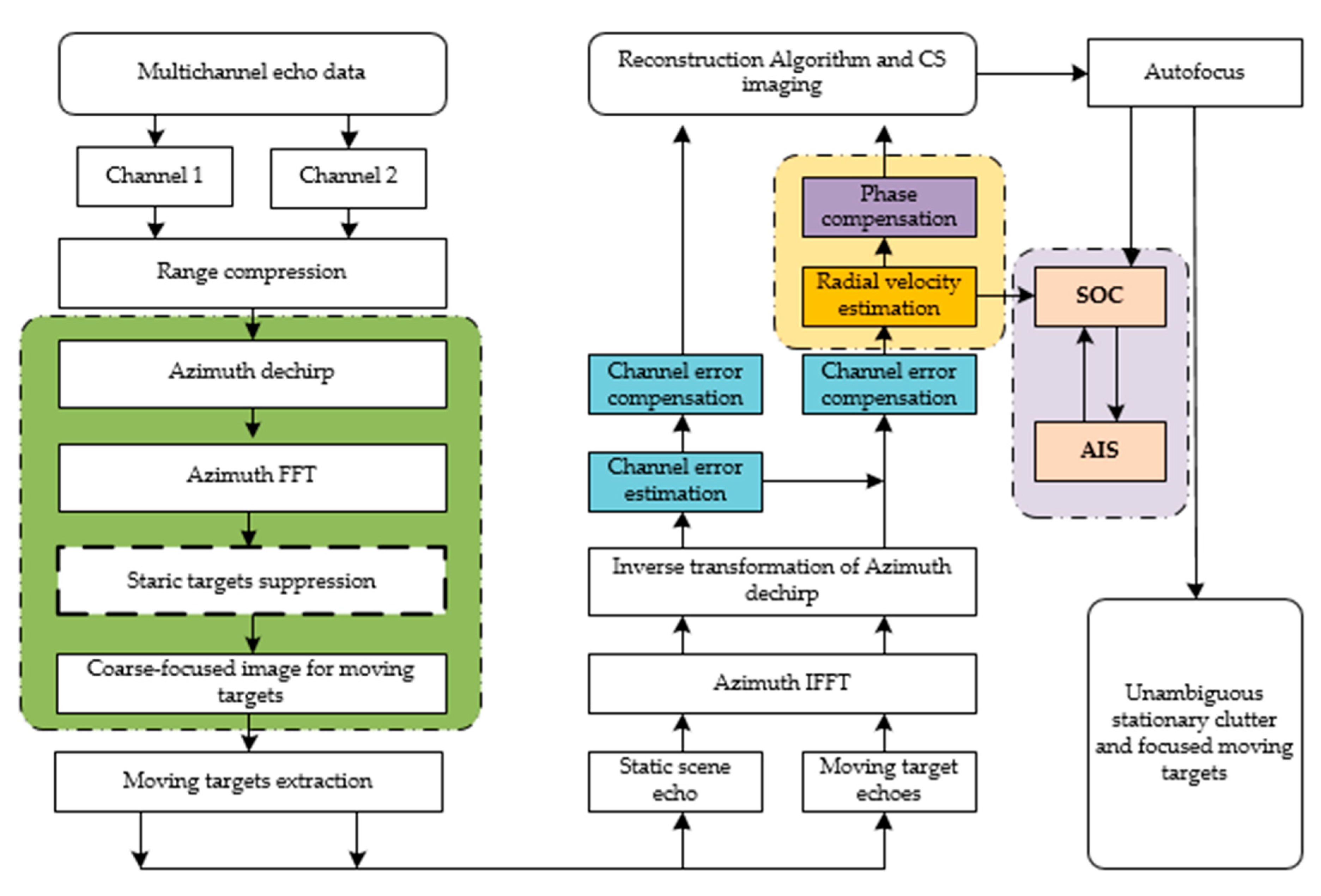
3. Processing Method

The whole processing flow for the simultaneous imaging scheme is shown in Figure 4. In the first step, the moving target echoes are extracted from the stationary clutter. For the maritime scenarios, we adopted an effective and efficient approach to extract the moving targets. A coarse-focused image is obtained after range compression and an azimuth dechirp operation. In more practical applications, it is able to extract multiple moving targets without clutter suppression, which is marked with a dotted box. Then, both the static scene echo and the moving target echoes need to return to the range time-azimuth time domain in two steps. Since the estimation of the channel imbalance is affected by the moving targets, it is necessary to estimate the channel imbalance with the static scene echo. The estimated result is used to compensate the channel error of moving targets. In order to achieve simultaneous processing of static and moving targets, the phase terms introduced by radial velocity need to be compensated. Lastly, the moving targets echoes are added back to the stationary scene echo and an unambiguous image can be obtained by the reconstruction and the classical CS algorithm. The along-track velocity is calculated by the autofocus algorithm and speed over ground of the moving ship is confirmed by comparing the velocity in the AIS sensor data. Three crucial steps will be explained in detail below.

3.1. Extraction of the Moving Targets Echoes

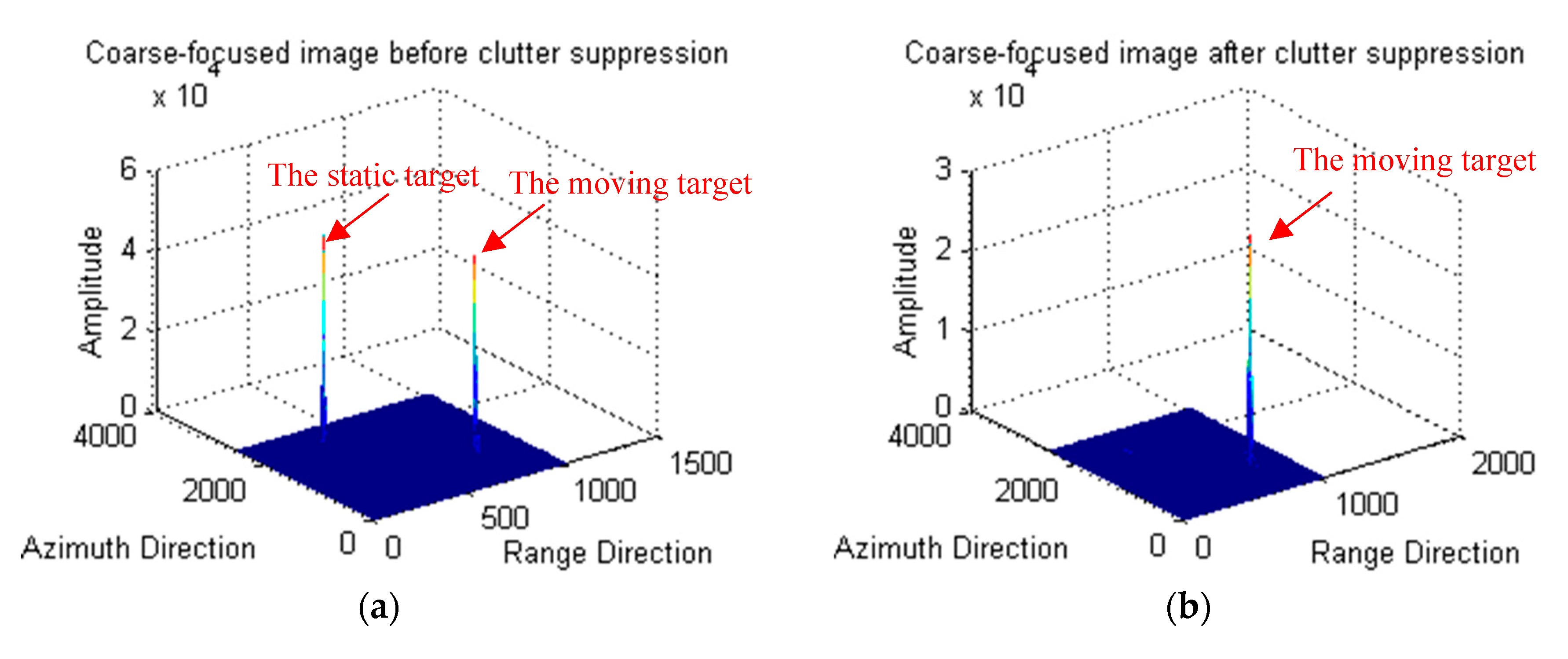
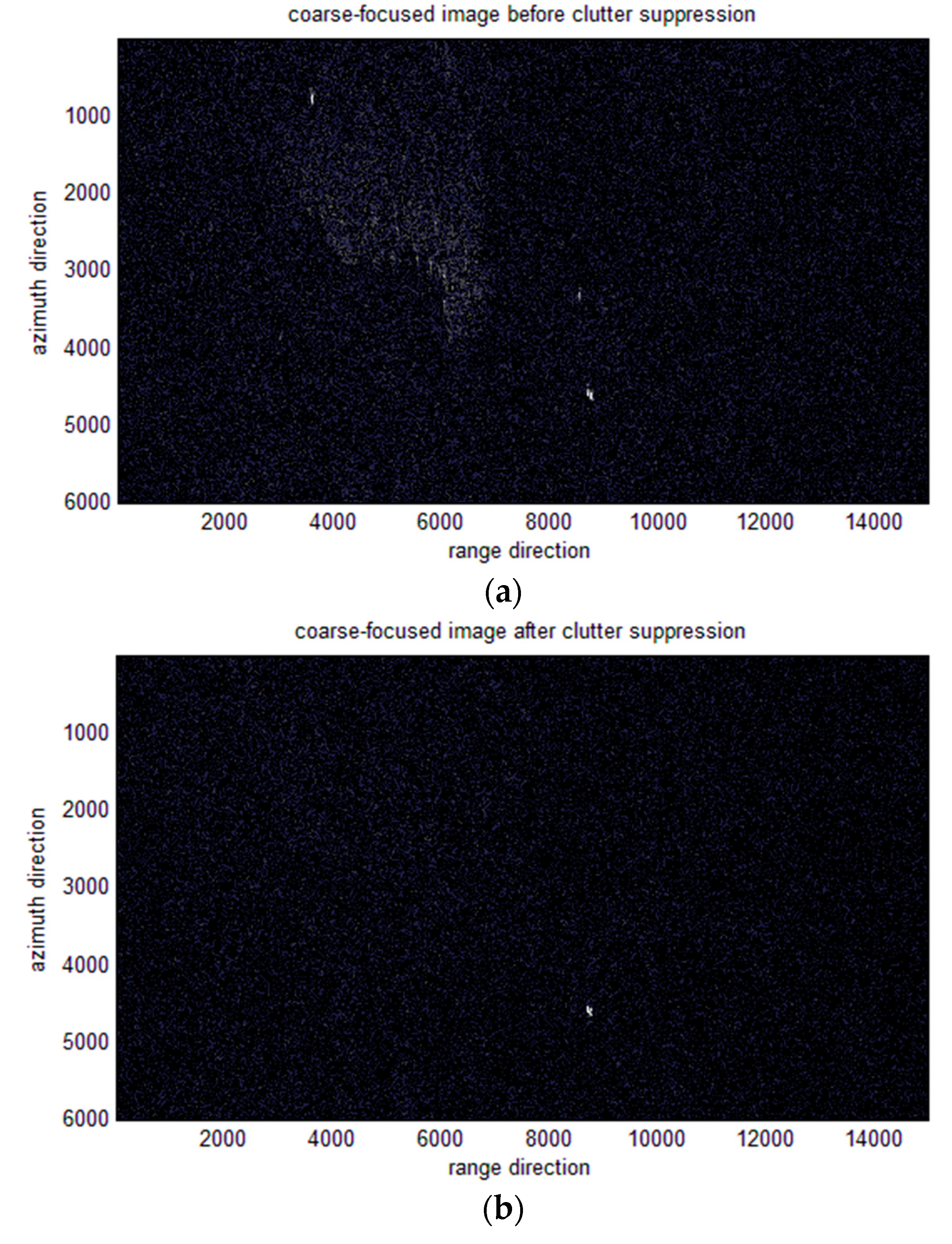
3.1.1. Stationary Targets Suppression

For most maritime scenarios, it is not necessary to suppress the stationary targets since moving targets are embedded in a rather weak clutter environment with strong signals. However, in some scenarios, such as the scene close to the coast or the scene with stalled ships, the stationary target suppression is particularly important.

For the convenience of expression, it is assumed that the moving target is at the center of the scene, i.e., ${\eta }_c=0$. The received signal of the $m$-th channel after range compression (RC) is given by:

$$S_{m\_rc}\left(\mathsf{\tau },\eta \right)=C_0·sinc\left\{\pi ·B·\left(\tau -\frac{2R_m\left(\eta \right)}{c}\right)\right\}·rect\left(\frac{\eta }{T_s}\right)·\exp \left\{-j\frac{4\pi R_m\left(\eta \right)}{\lambda }\right\},$$

(9)

where $C_0$ is also a complex constant and $B= K_r·T_p$ is the signal bandwidth. Substituting Equation (2) into Equation (9), $S_{m\_rc}\left(\mathsf{\tau },\mathsf{\eta }\right)$ can be expanded as follows:

$$S_{m\_rc}\left(\mathsf{\tau },\mathsf{\eta }\right)=C_0·sinc\left\{\pi ·B·\left(\tau -\frac{2R_m\left(\mathsf{\eta }\right)}{c}\right)\right\}·rect\left(\frac{\mathsf{\eta }}{T_s}\right)·\exp \left\{j\pi K_a{\eta }^2+j2\pi f_{m\_dc}\eta -j\frac{4\pi R_0}{\lambda }\right\},$$

(10)

where $K_a$ and $f_{m\_dc}$ stand for the Doppler rate and the Doppler centroid of the $m$-th channel, respectively.

$$K_a=-\frac{2{\left(V_s-V_a\right)}^2}{\lambda R_0},$$

(11)

$$f_{m\_dc}=-\frac{2V_r}{\lambda }-\frac{2\left(V_s-V_a\right)·x_{m\_epc}}{\lambda R_0}.$$

(12)

It is noted in Equation (11) that the existence of the along-track velocity makes the Doppler rate of the moving target different from that of the stationary one, which will result in the moving target being unfocused. However, fortunately, the autofocus technology has solved the problem and, at the same time, the estimated result of the along-track velocity can be obtained. Thus, to pay high attention to the effects of the radial velocity, the along-track velocity is ignored in the following derivation. The Doppler rate becomes:

$$K_a=-\frac{2V_s^2}{\lambda R_0}.$$

(13)

It is illustrated in Equation (12) that the existence of radial velocity results in a shift in the Doppler centroid. As the along-track velocity $V_a$ is much smaller than the satellite, the Doppler centroid is expressed below.

$$f_{m\_dc}=-\frac{2V_r}{\lambda }-\frac{2V_s·x_{m\_epc}}{\lambda R_0}.$$

(14)

The azimuth dechirp operation is exploited to get the coarse-focused imaging, and the moving target indication can be achieved in the range time-azimuth dechirp frequency domain. The signal of the $m$-th channel after azimuth dechirp can be expressed as the equation below.

$$\begin{array}{cc}\hfill S_{m\_dechirp}\left(\mathsf{\tau },\mathsf{\eta }\right)& =S_{m\_rc}\left(\mathsf{\tau },\mathsf{\eta }\right)\ast S_{ref}\left(\eta \right)\hfill \\ & =C_0·sinc\left\{\pi ·B·\left(\tau -\frac{2R_m\left(\eta \right)}{c}\right)\right\}·rect\left(\frac{\eta }{T_s}\right)·\exp \{j2\pi f_{m_{\_dc}}·\eta -j\frac{4\pi R_0}{\lambda }\},\hfill \end{array}$$

(15)

and the reference function can be written as:

$$S_{ref}\left(\eta \right)=\exp \left(-j\pi K_a{\eta }^2\right).$$

(16)

In order to suppress clutter, 1th-channel is shifted in the azimuth direction for $T_d$ matched with the second channel, where:

$$T_d=\frac{d}{2V_s}.$$

(17)

Substituting Equation (2), (3), and (14) into Equation (15), the shifted signal of the first channel can be written as:

$$\begin{array}{cc}\hfill S_{1\_dechirp}\left(\mathsf{\tau },\eta +T_d\right)& =C_0·sinc\left\{\pi ·B·\left(\tau -\frac{2R_2\left(\eta \right)}{c}-\frac{d·V_r}{c·V_s}\right)\right\}\hfill \\ & ·rect\left(\frac{\eta +T_d}{T_s}\right)·\exp \left(j2\pi f_{2\_dc}\eta -j\frac{4\pi R_0}{\lambda }-j\frac{2\pi ·d·V_r}{\lambda ·V_s}\right).\hfill \end{array}$$

(18)

In addition, the signal of the second channel can be expressed as:

$$S_{2\_dechirp}\left(\mathsf{\tau },\eta \right)=C_0·sinc\left\{\pi ·B·\left(\tau -\frac{2R_2\left(\mathsf{\eta }\right)}{c}\right)\right\}·rect\left(\frac{\eta }{T_s}\right)·\exp \left(j2\pi f_{2\_dc}\mathsf{\eta }-j\frac{4\pi R_0}{\lambda }\right).$$

(19)

At this point, the data of the two channels match in azimuth time, and the result of subtraction is given as follows.

$$\begin{array}{cc}\hfill S_{sub}\left(\mathsf{\tau },\mathsf{\eta }\right)& =S_{1_{dechirp}}\left(\mathsf{\tau },\mathsf{\eta }+T_d\right)-S_{2_{dechirp}}\left(\mathsf{\tau },\mathsf{\eta }\right)\hfill \\ & =C_0·rect\left(\frac{\mathsf{\eta }}{T_s}\right)·\exp \left(j2\pi f_{2\_dc}\mathsf{\eta } -j\frac{4\pi R_0}{\lambda }\right)·t\left(\tau ,\mathsf{\eta },V_r\right),\hfill \end{array}$$

(20)

where

$$\begin{array}{cc}\hfill t\left(\tau ,\mathsf{\eta },V_r\right)& =sinc\left\{\pi ·B·\left(\tau -\frac{2R_2\left(\mathsf{\eta }\right)}{c}-\frac{d·V_r}{c·V_s}\right)\right\}\hfill \\ & ·\exp \left(-j\frac{2\pi ·d·V_r}{\lambda ·V_s}\right)-sinc\left\{\pi ·B·\left(\tau -\frac{2R_2\left(\mathsf{\eta }\right)}{c}\right)\right\}.\hfill \end{array}$$

(21)

From Equations (20) and (21), for the stationary target without radial velocity, the result of Equation (20) is zero, which means the stationary target is suppressed, while, for the moving target, Equation (20) almost becomes a single-frequency signal. Thus, after Fourier transform along the azimuth, there will be energy around the specific frequency point. The range time-azimuth dechirp frequency domain representation of Equation (20) is given below.

$$S_{m\_dechirp}\left(\mathsf{\tau },f_a\right)=C_0·T_s·sinc\left(T_s\left(f_a-f_{2_{dc}}\right)\right)·\exp \left(-j\frac{4\pi R_0}{\lambda }\right)\ast T\left(\tau ,f_a,V_r\right).$$

(22)

where $\{\ast \}$ denotes the convolution operation and $T\left(\tau ,f_a,V_r\right)$ is the Fourier transform of Equation (21). The moving target echoes can be extracted on the coarse-focused imaging later.

3.1.2. Extraction of the Moving Target Echoes

In the above derivation, we focused on the suppression of stationary targets. Thus, the only target in the center of the scene is considered. However, in more practical applications, it is able to simultaneously extract multiple moving targets that are sparsely distributed in the scene without clutter suppression. The signal of the $m$-th channel after azimuth dechirp for the moving target at azimuth position $X_0$ can be expressed as:

$$\begin{array}{cc}\hfill S_{m\_dechirp}\left(\mathsf{\tau },\eta -{\eta }_c\right)& =S_{m\_rc}\left(\mathsf{\tau },\eta -{\eta }_c\right)\ast S_{ref}\left(\eta \right)\hfill \\ & =C_0·sinc\left\{\pi ·B·\left(\tau -\frac{2R_m\left(\eta -{\eta }_c\right)}{c}\right)\right\}·rect\left(\frac{\eta -{\eta }_c}{T_s}\right)\hfill \\ & ·\exp \left\{-j2\pi K_a{\eta }_c·\eta +j2\pi f_{m\_dc}·\eta +j\phi \right\},\hfill \end{array}$$

(23)

where

$$\phi =-\frac{4\pi R_0}{\lambda }-2\pi f_{m\_dc}{\eta }_c+\pi K_a{\eta }_c{}^2.$$

(24)

After Fourier transform along the azimuth, Equation (23) becomes:

$$\begin{array}{cc}\hfill S_{m\_dechirp}\left(\mathsf{\tau },f_a\right)& =C_0·T_s·sinc\left\{\pi ·B·\left(\tau -\frac{2R_m\left(f_a\right)}{c}\right)\right\}\hfill \\ & ·sinc\left(T_s\left(f_a+K_a{\eta }_c-f_{m\_dc}\right)\right)·\exp \left(-j2\pi f_a·{\eta }_c\right)·\exp \left(j\varphi \right).\hfill \end{array}$$

(25)

From Equation (25), a coarse-focused image is obtained in a range of the time-azimuth dechirp frequency domain with moving targets. However, a low PRF is adopted for the HRWS SAR system. Thus, the signal with the Doppler ambiguity is expressed as:

$$\begin{array}{cc}\hfill S_{m_{dechirp}}\left(\mathsf{\tau },f_a\right)& ={\displaystyle {\displaystyle \sum }_{I=-\frac{\left(N-1\right)}{2}}^{\frac{\left(N-1\right)}{2}}}{C}_0·sinc\left\{\pi ·B·\left(\tau -\frac{2R_m\left(f_a\right)}{c}\right)\right\}·T_s\hfill \\ & ·sinc\left(T_s\left(f_a+K_a{\eta }_c-f_{m_{\_dc}}+i·PRF\right)\right)·\exp \left(-j2\pi f_a·{\eta }_c\right)·\exp \left(j\varphi \right),\hfill \\ & \hfill (-\frac{PRF}{2}\le f_a\le \frac{PRF}{2})\end{array}$$

(26)

where $\mathrm{N}$ is the number of the main Doppler spectrum ambiguity.

It can be clearly seen from Equation (26) that the moving target is roughly focused on the azimuth frequency of $f_a=-K_a{\eta }_c+f_{m\_dc}$ if there is no Doppler ambiguity. Substituting Equations (13) and (14), the expression of the azimuth frequency is given by the equation below.

$$f_a\approx \frac{2V_s^2}{\lambda R_0}{\eta }_c-\frac{2V_r}{\lambda }.$$

(27)

We have made a reasonable approximation of the result in this scenario because $x_{m\_epc}\ll R_0$. Only when $\left|f_a\right|<PRF/2$, the position where the target appears will not be folded. Otherwise, the scene will fold into the range of $-PRF/2$ to $PRF/2$. It is noticeable, however, that no false targets will appear. From Equation (26), one can draw a conclusion that the moving targets with different radial velocities at different azimuth positions will be coarsely focused at different frequency points.

3.2. Two Methods to Estimate Radial Velocity

After extracting the moving target echoes, each echo data needs to return to the range time-azimuth time domain in two steps:

1)

Azimuth inverse Fourier transform,

2)

Inverse transform of azimuth dechirp operation, where the reference function becomes

$$S_{ref}{}^{\ast }\left(\eta \right)=\exp \left(j\pi K_a{\eta }^2\right).$$

(28)

Since the estimation of the amplitude and phase errors between the channels is affected by the moving targets echoes, it is necessary that the channel imbalance is estimated with the stationary scene echo. The extracted moving target echo without channel imbalance returns to the range compressed signal, and the signal is expressed as Equation (10). In this paper, in order to make the scheme suitable for any SCR situation, the radial velocity is estimated using the TDC method and the ML-based algorithm proposed in Reference [10]. The estimation results of the two methods verify each other, and their performance comparison is given in the following section. The details of the two methods are discussed next.

3.2.1. TDC Method

For the DRC mode, the instantaneous slant range of each channel can be expressed as Equation (1). The azimuth time delay between the two effective phase centers is written as Equation (17). The delayed instantaneous slant range of the first channel is shown below.

$$R_1\left(\eta +T_d\right)=R_0+V_r\eta +\frac{{\left(V_s\eta +\frac{d}{4}\right)}^2}{2R_0}+T_d·V_r=R_2\left(\eta \right)+T_d·V_r.$$

(29)

The moving target echo of each channel is given by:

$$S_{1\_rc}\left(\mathsf{\tau },\eta +T_d\right)=C_0·sinc\left\{\pi ·B·\left(\tau -\frac{2R_1\left(\eta +T_d\right)}{c}\right)\right\}·rect\left(\frac{\mathsf{\eta }}{T_s}\right)·\exp \left\{-j\frac{4\pi R_2\left(\eta \right)}{\lambda }-j\frac{4\pi }{\lambda }·T_d·V_r\right\},$$

(30)

$$S_{2\_rc}\left(\mathsf{\tau },\mathsf{\eta }\right)=C_0·sinc\left\{\pi ·B·\left(\tau -\frac{2R_2\left(\mathsf{\eta }\right)}{c}\right)\right\}·rect\left(\frac{\mathsf{\eta }}{T_s}\right)·\exp \left\{-j\frac{4\pi R_2\left(\mathsf{\eta }\right)}{\lambda }\right\}.$$

(31)

Conjugate multiply the two echo data to obtain the interferometric phase, which is written as:

$$\mathsf{\phi }=angle\left\{S_{1_{rc}}\left(\mathsf{\tau },\eta +T_d\right)\ast S_{2_{rc}}{}^{\ast }\left(\mathsf{\tau },\mathsf{\eta }\right)\right\}=-\frac{4\pi }{\lambda }·T_d·V_r,$$

(32)

where the $angle\{\cdot \}$ function returns the phase of a complex signal. Then, the radial velocity can be calculated by the equation below.

$$V_r=-\mathsf{\phi }·\frac{\lambda }{4\pi ·T_d}.$$

(33)

3.2.2. ML-Based Algorithm

The existence of radial velocity cases shows a certain offset of the Doppler frequency and that the cone angle of the moving target for a certain Doppler bin is related to $V_r$. Since there is a one-to-one correspondence between radial velocity and the cone angle for a moving target, the ML algorithm transforms the velocity estimation problem to the cone angle estimation or the steering vector estimation. The steering vector matrix of a moving target for the DRC mode is shown below.

$$\mathit{A}\left(f_a\right)=\left[\begin{array}{ccc}\begin{array}{cc}{\mathit{\alpha }}_{\mathrm{t},-2}& {\mathit{\alpha }}_{\mathrm{t},-1}\end{array}& {\mathit{\alpha }}_{\mathrm{t},0}& \begin{array}{cc}{\mathit{\alpha }}_{\mathrm{t},1}& {\mathit{\alpha }}_{\mathrm{t},2}\end{array}\end{array}\right]$$

(34)

where ${\mathit{\alpha }}_{\mathrm{t},\mathrm{n}}$ denotes the n-th ambiguous steering vector, i.e.,

$${\mathit{\alpha }}_{\mathrm{t},\mathrm{n}}={\left[\begin{array}{cc}\exp \left(-j2\pi \left(f_a-n·PRF+\frac{2V_r}{\lambda }\right)·\frac{x_1}{2V_s}\right)& \exp \left(-j2\pi \left(f_a-n·PRF+\frac{2V_r}{\lambda }\right)·\frac{x_2}{2V_s}\right)\end{array}\right]}^{\mathrm{T}}.$$

(35)

In addition, $x_m$ denotes the displaced length of the $m$-th actual receive phase center from the array center in the along-track direction, which can be expressed as:

$$x_m=\left(\mathrm{m}-\frac{3}{2}\right)·\mathrm{d},\mathrm{m}=1,2.$$

(36)

The criterion of the ML estimator maximizes the following cost function.

$$F_{ML}\left(V_r\right)=tr\left[\mathit{I}-\mathit{A}{\left({\mathit{A}}^H\mathit{A}\right)}^{-1}{\mathit{A}}^H\right]{\mathit{R}}_X,$$

(37)

where $tr[·]$ represents the trace of a matrix, $\mathit{A}$ is the steering vector matrix in Equation (34), and ${\mathit{R}}_X$ is the signal covariance matrix. Sample the extracted signal echo in the range-Doppler domain at a certain Doppler bin $f_{a,k}$ to constitute vector $\mathit{X}$:

$$\mathit{X}={\left[S_{1\_rc}\left(\tau ,f_{a,k}\right) ,S_{2\_rc}\left(\tau ,f_{a,k}\right)\right]}^T.$$

(38)

The signal covariance matrix is acquired by the equation below.

$${\mathit{R}}_X=\mathit{X}·{\mathit{X}}^H.$$

(39)

By searching for $V_r$ and computing the steering vector matrix $\mathit{A}$, the maximum likelihood spectrum can be calculated. The maximum value of the spectrum corresponds to the ML estimation of $V_r$. In Reference [10], the authors average the estimated values from K Doppler bins to improve the robustness.

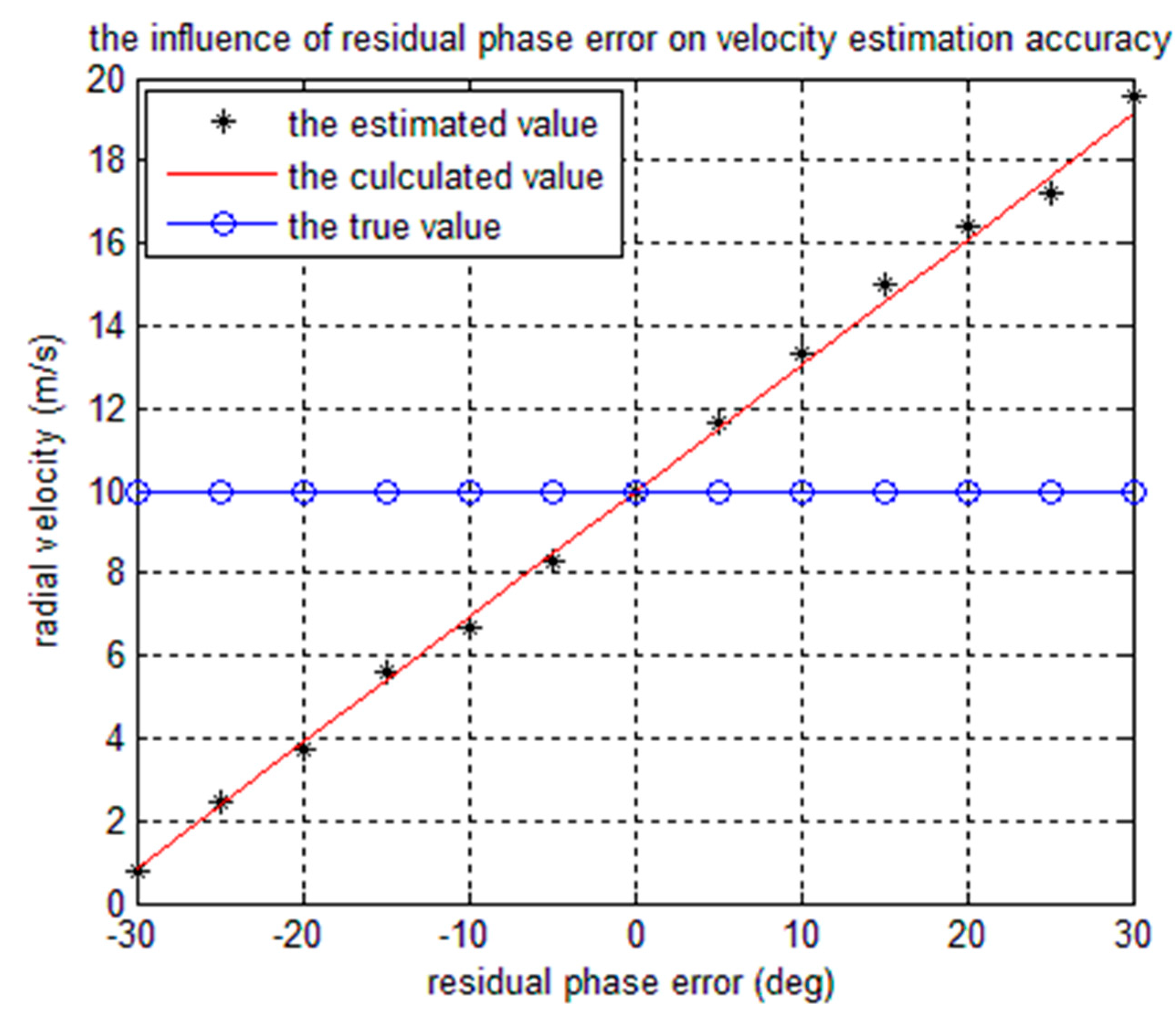
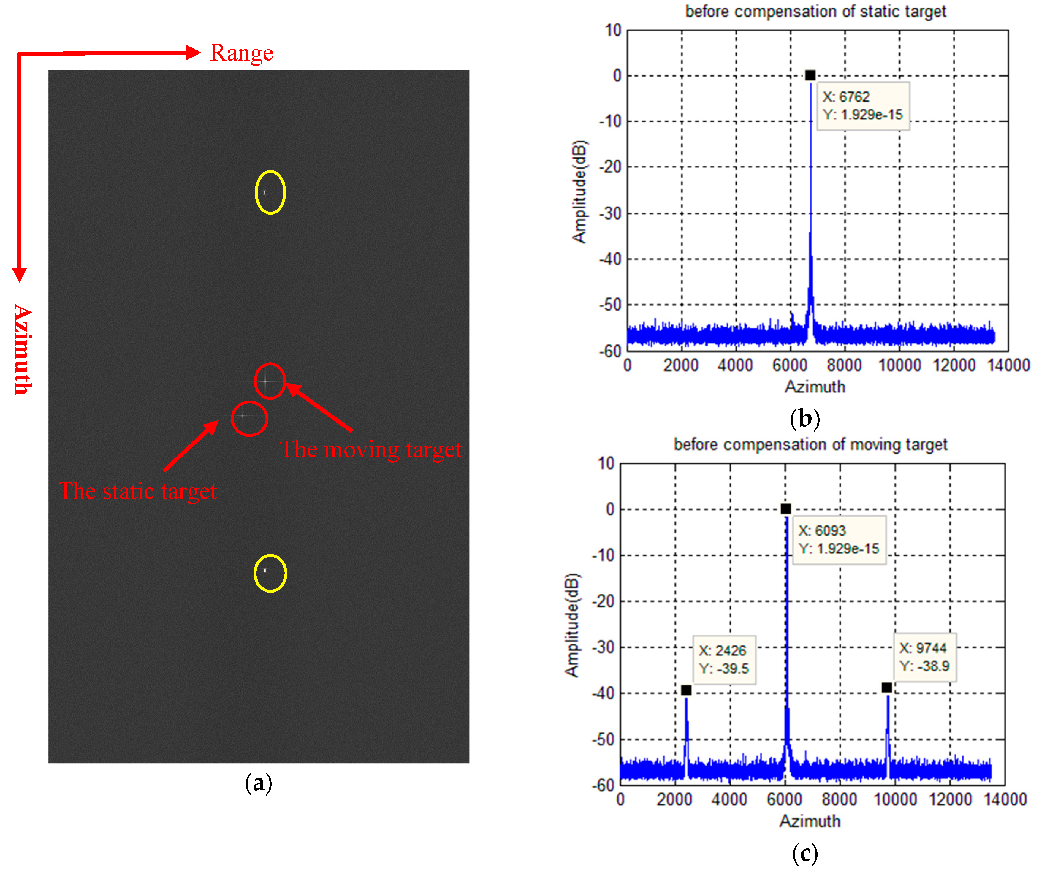
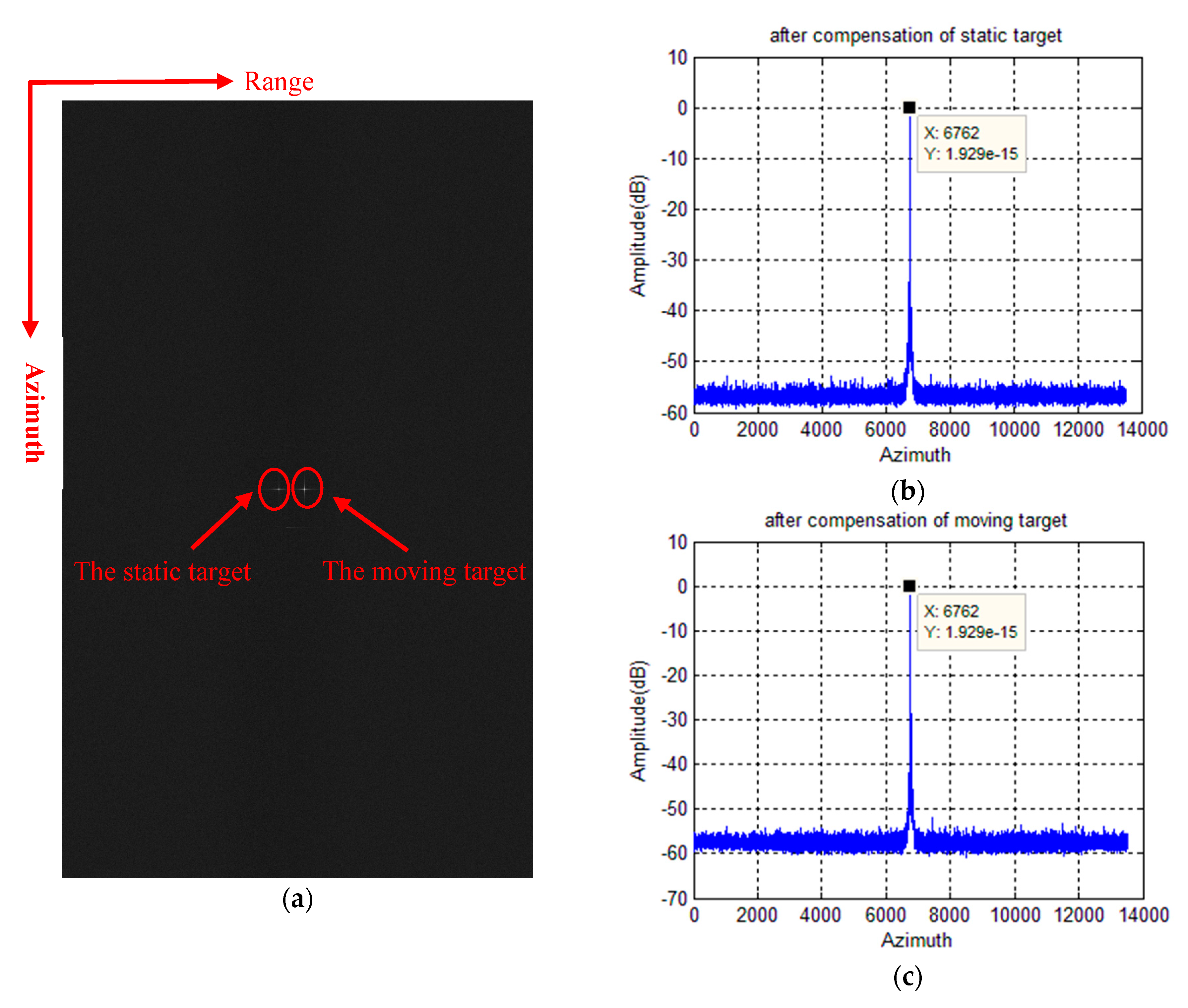
3.3. Compensation for the Phase Introduced by Radial Velocity

In order to achieve simultaneous processing of static and moving target echoes, the phase introduced due to the radial velocity needs to be compensated. Conduct the range Fourier transform to Equation (10) and the signal in range frequency-azimuth time domain of the $m$-th channel can be expressed by the equation below.

$$S_{m\_rc}\left(f_r,\mathsf{\eta }\right)=E_0·rect\left(\frac{\mathsf{\eta }}{T_s}\right)·\exp \left\{-j\frac{4\pi R_m\left(\mathsf{\eta }\right)}{c}·f_r\right\}·\exp \left\{j\pi K_a{\eta }^2+j2\pi f_{dc}\eta -j\frac{4\pi R_0}{\lambda }\right\},$$

(40)

where $E_0$ is also a complex constant. Substituting Equations (2) and (14) into Equation (40) gives the following.

$$\begin{array}{cc}\hfill S_{m\_rc}\left(f_r,\mathsf{\eta }\right)& =E_0·rect\left(\frac{\mathsf{\eta }}{T_s}\right) \cdot \exp \left\{-j\left(\frac{4\pi R_0}{c}+\frac{2\pi {\left(V_s\eta +·x_{m\_epc}\right)}^2}{c{R}_0}\right)·f_r-j2\pi \frac{2V_r\eta }{c}·f_r\right\}\hfill \\ & ·\exp \left\{j\pi K_a{\eta }^2-j2\pi \frac{2V_s·x_{m\_epc}}{\lambda R_0}\eta -j\frac{4\pi R_0}{\lambda }-j2\pi \frac{2V_r}{\lambda }\eta \right\},\hfill \end{array}$$

(41)

while for a static target, $V_r=0$, the expression becomes the following.

$$\begin{array}{cc}\hfill S_{m\_rc\_s}\left(f_r,\mathsf{\eta }\right)& =E_0·rect\left(\frac{\mathsf{\eta }}{T_s}\right) \cdot \exp \left\{-j\left(\frac{4\pi R_0}{c}+\frac{2\pi {\left(V_s\eta +x_{m\_epc}\right)}^2}{c{R}_0}\right)·f_r\right\}\hfill \\ & ·\exp \left\{j\pi K_a{\eta }^2-j2\pi \frac{2V_s·x_{m\_epc}}{\lambda R_0}\eta -j\frac{4\pi R_0}{\lambda }\right\}.\hfill \end{array}$$

(42)

Clearly, the relationship between Equations (41) and (42) is given by the formula below.

$$S_{m\_rc}\left(f_r,\mathsf{\eta }\right)=S_{m\_rc\_s}\left(f_r,\mathsf{\eta }\right)·\exp \left(-j2\pi \frac{2V_r\eta }{c}·f_r\right)·\exp \left(-j2\pi \frac{2V_r}{\lambda }\eta \right).$$

(43)

From Equation (43), there are two terms caused by radial velocity. The first term is the linear component of range cell migration (RCM) for the moving target, and the second one is an offset of the Doppler frequency. The compensation function is employed to eliminate the difference between static scene echoes and moving target echoes, which can be defined as the equation below.

$$S_{com}\left(f_r,\mathsf{\eta }\right)=\exp \left(j2\pi \frac{2V_r\eta }{c}·f_r\right)·\exp \left(j2\pi \frac{2V_r}{\lambda }\eta \right).$$

(44)

After multiplying by the compensation function, the moving target echoes are added back to the stationary scene echo. Lastly, an unambiguous image can be obtained by the reconstruction algorithm and the classical CS algorithm.

4. Experimental Results

In this section, an experiment is conducted first to compare the performance of the TDC method and ML-based algorithm. Then, simulated DRC SAR data experiments are employed to evaluate the performance of moving targets detection and extraction, radial velocity estimation, and compensation for the moving target echoes. Eventually, real data of the GF-3 DRC mode are adopted to verify the method mentioned above.

4.1. Performance Comparison of Two Radial Velocity Estimation Methods

In order to compare the performance of the TDC method and the ML-based algorithm, an experiment is conducted to evaluate the estimation accuracy under different Signal-to-Clutter Ratios (SCR). Since the two radial velocity estimation methods are applied to the range-compressed echo, the clutter is added to the echo after range compressing. In his experiment, the true value of the radial velocity of the moving target is 10 m/s, and the SCR varies from 0 $\mathrm{dB}$ to 20 $\mathrm{dB}$. Ten experiments were performed under each SCR, where the maximum estimation error (MEE) means the result with the largest deviation from the true value. The average of 10 results is used to calculate the average estimation error (AEE). The estimation errors under different SCRs of the two radial velocity estimation methods are listed in

Table 1. Estimation errors under different SCRs of the TDC method.

SCR(dB)	20	15	10	5	0
MEE	0.461%	0.704%	1.698%	2.434%	6.172%
AEE	0.033%	0.110%	0.246%	0.750%	2.454%

and

Table 2. Estimation errors under different SCRs of the ML-based algorithm.

SCR(dB)	20	15	10	5	0
MEE	0.391%	0.432%	0.851%	1.286%	5.041%
AEE	0.004%	0.078%	0.114%	0.321%	2.296%

.

In a sense, the average of multiple experimental results can improve accuracy as much as possible, while the estimation error of a certain experiment will not exceed the MEE. From the results in Table 1 and Table 2, the ML-based algorithm shows better performance than the TDC method under various SCRs. However, the ML-based algorithm is less efficient since it needs to search for the radial velocity at some azimuth frequency points. As long as the energy of the clutter is no stronger than that of the signal in the echo domain, i.e., the SCR is larger than 0 $\mathrm{dB}$, both the TDC method and the ML-based algorithm can obtain an effective estimated result. When the clutter energy is almost equal to the signal energy, the MEE of the two methods is greater than 5%. However, the MEE of the ML-based algorithm is almost twice as small as the MEE of the TDC method when the SCR is greater than 5 $\mathrm{dB}$ and less than 15 $\mathrm{dB}$. Under the condition that the clutter is relatively weak, although the MEE of the ML-based algorithm is smaller, considering the efficiency problem, the TDC method is preferentially selected to estimate the radial velocity. In this paper, when the results of the two methods are obtained at the same time without considering the efficiency, the estimated result of the ML-based algorithm is preferentially utilized to compensate for the phase. The result of the TDC method evaluates the validity of the estimated results of the ML-based algorithm since it is credible that the two results of the two methods with completely different principles are similar to each other. However, in practice, we prefer the TDC method to estimate the radial velocity under a high SCR with an acceptable error due to high efficiency.

However, the accuracy of the estimated velocity is affected by many factors, such as residual phase error between channels. Before the velocity estimation, the amplitude and phase error between the channels is estimated and compensated, as shown in Figure 4. If there is a residual phase error, it will affect the speed estimation result. For the TDC method, the interferometric phase with the residual phase error can be written as the equation below.

$$\widehat{\mathsf{\phi }}=-\frac{4\pi }{\lambda }·T_d·V_r+{\phi }_{error},$$

(45)

In addition, the estimated velocity can be expressed by the formula below.

$$\widehat{V_r}=V_r\pm \left|{\phi }_{error}·\frac{\lambda }{4\pi T_d}\right|.$$

(46)

The influence of the residual phase error on velocity estimation accuracy is shown in Figure 5. The true value of the radial velocity is 10 m/s. The calculated value is obtained, according to Equation (46), while the estimated value is the result of the TDC method. In the DRC mode of GF-3, the residual phase error per 1 degree will bring an error of 0.3049 m/s to the radial velocity estimation result.

4.2. Simulation Experiment

The simulation experiments of the DRC mode are carried out according to the GF-3 satellite parameters shown in

Table 3. Simulation parameters.

Parameter	Symbol	Value
Pulse repetition frequency	PRF	3953.857910 Hz
The length of the antenna	Da	7.5 m
Platform Velocity	$V_s$	7546.671805 m/s
Sample Frequency	$F_s$	133.33 MHz
Bandwidth	$B$	100 MHz
Pulse width	$T_p$	55 us
Wavelength	$\lambda$	0.055517 m
Doppler Bandwidth	$B_a$	2470.53 Hz
Doppler Rate	$K_a$	−1910.36 Hz/s

. The simulated echo data without channel imbalance is designed to make static targets unambiguous for convenience. In the experiment, there is a static target and a moving target whose radial velocity is 10 m/s and the along-track velocity is not taken into account in this case. It should be emphasized that they are in the same azimuth position but at different range bins.

In this case, we present the imaging result of simulated echo data without any operation on the moving target in Figure 6a. The main targets are circled in red, while the false targets of the moving target are in the yellow circles. False targets will arise along the azimuth direction in the imaging results if the moving target is addressed along with the static one. The azimuth profiles of imaging results are shown in Figure 6b,c, which correspond to the azimuth profiles of the static target and the moving target in Figure 6a, respectively. The maximum power of false targets relative to the real one is −38.9 $\mathrm{dB}$. From Figure 6, the moving target is focused on the incorrect azimuth position since it should be the same as the static target.

The first channel data is transformed into the range time-azimuth dechirp frequency domain to obtain a coarse-focused image shown in Figure 7a, which includes both the moving target and the static target. However, when we subtract the data of two channels after registration, the static target is suppressed, as shown in Figure 7b.

The extracted moving target echo transformed inversely into a range-compressed echo is exploited to estimate the radial velocity. In this experiment, the estimated result of the TDC method is 10.0056 m/s, while that of the ML-based algorithm is 10.0016 m/s. Given the low noise energy, the estimation results of the two algorithms are very accurate. After compensation for the phase caused by radial velocity, the traditional CS algorithm is applied to the moving target echo along with the static scene echo. Lastly, the imaging results are in Figure 8a, and Figure 8b corresponds to the profile of the static target, while Figure 8c corresponds to the profile of the moving target in Figure 8a. The maximum power of false targets has been suppressed to drown in the noise. The target returns to the correct position along the azimuth direction.

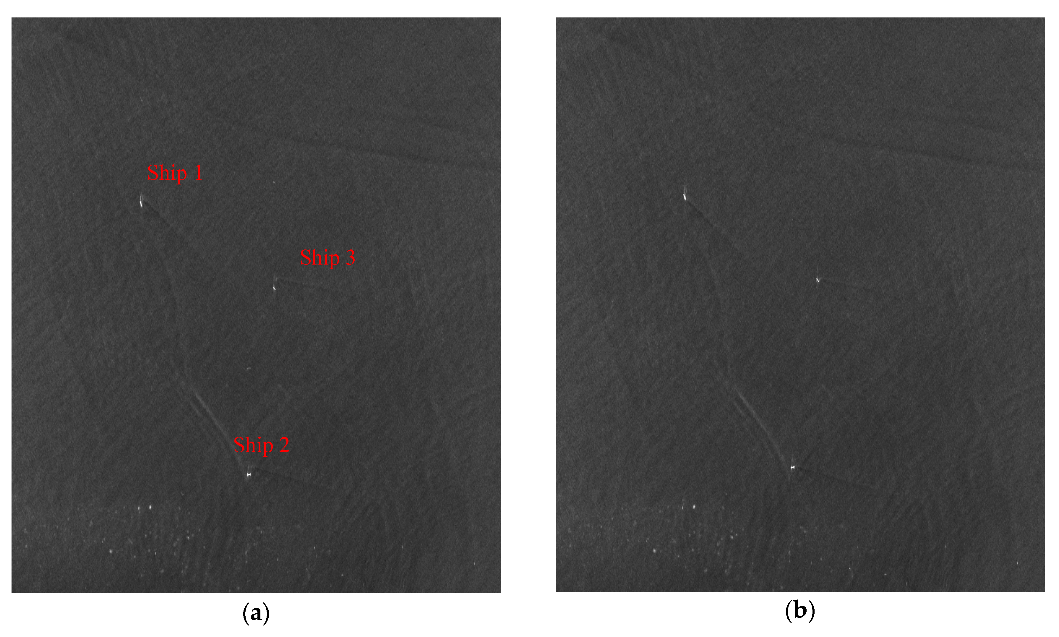
4.3. Real Data of GF-3

The proposed method of simultaneous imaging of stationary clutter and moving targets is applied to real data of GF-3. We selected two typical maritime scenes with one or more moving vessels to verify the proposed method.

In the first maritime scene, there is only one moving ship. The coarse-focused image after azimuth dechirp is shown in Figure 9a. It is impossible to firmly determine which strong point target is the vessel under the influence of the scene folding. Therefore, stationary target suppression is necessary. It can be seen from Figure 9b that the moving vessel was extracted after the clutter was suppressed. The estimated radial velocities of the TDC method and ML-based algorithm are –5.78 m/s and –5.82 m/s, respectively. (The direction of radial velocity along the range direction is positive.) Since the SCR in this experiment is 20.0345 $\mathrm{dB}$, the two results are highly accurate, according to Table 1 and Table 2. Regardless of efficiency, we take –5.82 m/s as the result to compensate for the phase term introduced by the radial velocity. The image before compensating for the moving target echo is shown in Figure 10a. Similarly, the red circle contains the real ship target and three false targets visible to the naked eye are circled with the yellow circle, and the imaging result after compensating for the phase term is shown in Figure 10b. Comparing Figure 10c,d, the false targets are suppressed so that they are submerged in the clutter and cannot be recognized.

Fortunately, the AIS information of the ship that coincided with the imaging time of Figure 10 was successfully obtained. It is shown that the ship’s speed over ground (SOG) is 20 knots, which means 10.27 m/s, and the course over ground (COG) is 240 degrees relative to the north. The estimated radial velocity of the ship in Figure 10 is −5.82 m/s, and the incidence angle at the ship is 40.5 degrees. Thus, the cross-track velocity on the ground $V_{rg}$ is 8.9615 m/s calculated by Equation (1). The along-track velocity is −5.1751 m/s obtained by autofocus technology [27,28] shown in Figure 11. (The direction of the along-track velocity along the azimuth direction is positive.) Combined with the two components of the velocity of the moving target, the speed of the ship on the ocean surface in Figure 10 is 10.35 m/s, which is only 0.08 m/s deviation from 10.27 m/s given by AIS information.

In the case of high clutter energy in maritime scenes, false targets are sometimes not easily identified. Nevertheless, judging from the trajectory of the ship on the image, the ship deviated from the correct position. First, the echoes of the three ships need to be extracted. However, due to the interference in the lower part of the scene and the folding of the scene, it is not easy to directly identify the moving target on the coarse-focused image shown in Figure 12a. The result of clutter suppression in Figure 12b tells which target is the moving one.

In Figure 13b, the ships return to the right position, which means it is focused on its trajectory, by compensating the phase related to the radial velocity. The estimated results of the two methods are listed in

Table 4. The estimated radial velocities of two methods.

Ship ID	TDC	ML	SCR
Ship 1	−3.84 m/s	−3.89 m/s	12.6994 dB
Ship 2	−3.36 m/s	−3.54 m/s	12.6867 dB
Ship 3	−4.49 m/s	−4.51 m/s	12.9757 dB

. The result of the autofocus technology about the three ships in Figure 13 is shown in Figure 14.

5. Discussion

The experimental results in Section 4 demonstrate the effectiveness of the proposed method of integration of moving target detection, velocity estimation, location, and simultaneous imaging for both the static scene and moving targets. These experiments focus on the processing of moving targets in the echo domain since the channel imbalance has been compensated and the non-uniform sampling problem of the stationary scene will be solved in the final step simultaneously with the compensated moving target echoes. From the imaging results in Figure 9, Figure 10, Figure 11, Figure 12, Figure 13 and Figure 14, there is little ambiguity in the whole scene for both the static scene and the moving targets after processing.

It is vital to estimate radial velocity accurately for the false targets suppression and relocation of the moving targets. In experiments with real data, we evaluate the validity of the estimated results in the following ways. (1) If the estimation results of the two methods working on completely different principles are similar, the results are considered reliable. (2) If the false targets of the moving targets are submerged in the clutter from the processed image, the estimated results are accepted. (3) If the moving targets on the ocean scene are focused on the right position after compensation judging from the trajectory, it is believable that the estimated result is close to the true value. (4) Combined with the AIS sensor data, which contain velocity information about the ship, the estimated result can be verified directly. It is a time-consuming task to find the AIS information of each ship on the corresponding image. The first three methods are preferred schemes used to verify whether the result is reliable.

In addition, extracting the moving targets echoes in the range time-azimuth dechirp frequency domain has some restrictions on the scene due to the targets folding, according to Equation (26). For some scenarios with a few vessels such as scene 1 and scene 2 used in Section 4.3, even if the scene is folded, the sparse distribution of vessels does not affect the echo extraction. However, if there are many vessels in the scene and the synthetic aperture lasts a long time, the folding of the scene may cause the vessels with different velocity and position to focus on the same azimuth frequency point. This problem greatly affects the performance of the moving target detection. We can also derive the condition that satisfies the non-folding scene referring to Equation (26). The azimuth time limitation of deviation from the center is given by the formula below.

$$|∆{\eta }_c|<\frac{PRF·\lambda R_0}{4V_s^2}.$$

(47)

Thus, for the scene with a great deal of moving vessels, the echo should be divided into several segments, according to the synthetic aperture time. In addition, each segment is also processed with the proposed scheme.

In summary of the above two points, the quality of the results depends on two aspects. One is the accuracy of the radial velocity estimation, and the other is the limitation of the scene. The accuracy of the radial velocity estimation is affected by many factors, such as the residual phase error between channels mentioned in Section 4.1, the moving ships’ shaking with the waves, and more. If the estimated result is not accurate, the false targets cannot be completely suppressed, and the processing result will be poor. On the other hand, the complexity of the scenario affects the outcome. If there are multiple islands in the scene or multiple ships in the same range bin, the difficulty of processing will be greatly increased.

6. Conclusions

In this paper, a simultaneous imaging scheme of stationary clutter and moving targets for maritime scenarios is proposed to obtain an unambiguous image based on the first Chinese dual-receive channel SAR sensor. The azimuth ambiguity of the stationary scene can be eliminated by correcting amplitude and phase imbalance between channels and the reconstruction algorithm, while the false targets of the moving target are suppressed by compensating the phase result from the radial velocity. Moving target echoes need to be detected and extracted first on the coarse-focused imaging prior to estimating the radial velocity. The TDC method and ML-based algorithm working in the echo domain are utilized to estimate radial velocity. After that, the compensated moving target echoes along with a stationary scene echo are reconstructed to obtain an unambiguous SAR image with moving targets relocated in the correct azimuth position. The experimental results show the effectiveness of the imaging scheme. Moreover, the AIS sensor information is employed to verify the estimated result. The proposed procedure has great potential for application in future HRWS SAR systems.

References

1. Currie, A.; Brown, M.A. Wide-swath SAR. IEE Proc. F Radar Signal Process. 1992, 139, 122–135. [Google Scholar] [CrossRef]
2. Gebert, N.; Krieger, G.; Moreira, A. Digital beamforming on receive: Techniques and optimization strategies or high-resolution wideswath SAR imaging. IEEE Trans. Aerosp. Electron. Syst. 2009, 45, 564–592. [Google Scholar] [CrossRef]
3. Han, B.; Ding, C.; Zhong, L.; Liu, J.; Qiu, X.; Hu, Y.; Lei, B. The GF-3 SAR data processor. Sensors 2018, 18, 835. [Google Scholar] [CrossRef] [PubMed]
4. Sun, J.; Yu, W.; Deng, Y. The SAR payload design and performance for the GF-3 mission. Sensors 2017, 17, 2419. [Google Scholar] [CrossRef] [PubMed]
5. Shang, M.; Qiu, X.; Han, B.; Ding, C.; Hu, Y. Channel imbalances and along-track baseline estimation for the GF-3 azimuth multichannel mode. Remote Sens. 2019, 11, 1297. [Google Scholar] [CrossRef]
6. Sun, G.; Xiang, J.; Xing, M.; Yang, J.; Guo, L. A channel phase error correction method based on joint quality function of GF-3 SAR dual-channel images. Sensors 2017, 18, 3131. [Google Scholar] [CrossRef] [PubMed]
7. Yang, T.; Li, Z.; Liu, Y.; Bao, Z. Channel error estimation methods for multichannel SAR systems in azimuth. IEEE Geosci. Remote Sens. Lett. 2013, 10, 548–552. [Google Scholar] [CrossRef]
8. Krieger, G.; Gebert, N.; Moreira, A. Unambiguous SAR signal reconstruction from nonuniform displaced phase center sampling. IEEE Geosci. Remote Sens. Lett. 2004, 1, 260–264. [Google Scholar] [CrossRef]
9. Kim, J.; Younis, M.; Prats, P.; Gabele, M.; Krieger, G. First spaceborne demonstration of digital beamforming for azimuth ambiguity suppression. IEEE Trans. Geosci. Remote Sens. 2013, 51, 579–590. [Google Scholar] [CrossRef]
10. Jin, T.; Qiu, X.; Hu, D.; Ding, C. An ML-based radial velocity estimation algorithm for moving targets in spaceborne high-resolution and wide-swath SAR systems. Remote Sens. 2017, 9, 404. [Google Scholar] [CrossRef]
11. Jin, T.; Qiu, X.; Hu, D.; Ding, C. Unambiguous imaging of static scenes and moving targets with the first Chinese dual-channel spaceborne SAR sensor. Sensors 2017, 17, 1709. [Google Scholar] [CrossRef] [PubMed]
12. Li, X.; Xing, M.; Xia, X. Simultaneous stationary scene imaging and ground moving target indication for high-resolution wide-swath SAR system. IEEE Trans. Geosci. Remote Sens. 2016, 54, 4224–4239. [Google Scholar] [CrossRef]
13. Tan, W.; Xu, W.; Huang, P.; Huang, Z.; Qi, Y.; Han, K. Investigation of azimuth multichannel reconstruction for moving targets in high resolution wide swath SAR. Sensors 2017, 17, 1270. [Google Scholar] [CrossRef]
14. Lightstone, L.; Faubert, D.; Rempel, G. Multiple phase centre DPCA for airborne radar. In Proceedings of the 1991 IEEE National, Los Angeles, CA, USA, 12–13 March 1991. [Google Scholar]
15. Gierull, C.H.; Sikaneta, I.H. Raw Data based two-aperture SAR ground moving target indication. In Proceedings of the IEEE 2003 International Geoscience and Remote Sensing Symposium (IGARSS 2003), Toulouse, France, 21–25 July 2003. [Google Scholar]
16. Wang, X.; Gao, G.; Zhou, S.; Zou, H. A clutter suppression approach for SAR-GMTI based on dual-channel DPCA. J. Radars. 2014, 3, 241–248. [Google Scholar]
17. Gierull, C.H. Statistical analysis of multilook SAR interferograms for CFAR detection of ground moving targets. IEEE Trans. Geosci. Remote Sens. 2004, 42, 691–701. [Google Scholar] [CrossRef]
18. Gierull, C.H.; Sikaneta, I.; Cerutti-Maori, D. Two-step detector for RADARSAT-2’s experimental GMTI mode. IEEE Trans. Geosci. Remote Sens. 2013, 51, 436–454. [Google Scholar] [CrossRef]
19. Klemm, R. Principles of Space-Time Adaptive Processing; IEE Publishers: London, UK, 2002. [Google Scholar]
20. Blunt, S.D.; Gerlach, K.; Rangaswamy, M. STAP using knowledge-aided covariance estimation and the FRACTA algorithm. IEEE Trans. Aerosp. Electron. Syst. 2006, 42, 1043–1057. [Google Scholar] [CrossRef]
21. Baumgartner, S.V.; Krieger, G. Simultaneous high-resolution wide-swath SAR imaging and ground moving target indication: Processing approaches and system concepts. IEEE J. Sel. Top. Appl. Earth Obs. Remote Sens. 2015, 8, 5015–5029. [Google Scholar] [CrossRef]
22. Zhang, S.; Xing, M.; Xia, X. Robust clutter suppression and moving target imaging approach for multichannel in azimuth high-resolution and wide-swath synthetic aperture radar. IEEE Trans. Geosci. Remote Sens. 2015, 53, 687–709. [Google Scholar] [CrossRef]
23. Gierull, C.H. Ground moving target parameter estimation for two-channel SAR. IEE Proc. Radar Sonar Navig. 2006, 153, 224–233. [Google Scholar] [CrossRef]
24. Frasier, S.J.; Camps, A.J. Dual-beam interferometry for ocean surface current vector mapping. IEEE Trans. Geosci. Remote Sens. 2001, 39, 401–414. [Google Scholar] [CrossRef]
25. Yang, T.; Wang, Y.; Li, W. A moving target imaging algorithm for HRWS SAR/GMTI systems. IEEE Trans. Aerosp. Electron. Syst. 2017, 53, 1147–1157. [Google Scholar] [CrossRef]
26. Wang, X.; Wang, R.; Li, N.; Zhou, C. A velocity estimation method of moving target for SAR high-resolution wide-swath mode. In Proceedings of the IEEE 2016 International Geoscience and Remote Sensing Symposium (IGARSS 2016), Beijing, China, 10–15 July 2016. [Google Scholar]
27. Carrara, W.; Goodman, R.; Majewski, R. Spotlight Synthetic Aperture Radar: Signal Processing Algorithms; Artech House: Norwood, MA, USA, 1995. [Google Scholar]
28. Yun, Y.; Qi, X.; Li, N. Moving ship SAR imaging based on parameter estimation. J. Radars. 2016, 5, 326–332. [Google Scholar]
29. Hu, Q.; Jiang, Y.; Zhang, J.; Sun, X.; Zhang, S. Development of an automatic identification system autonomous positioning system. Sensors 2015, 15, 28574–28591. [Google Scholar] [CrossRef] [PubMed]
Figure 1. Imaging geometry model of the dual receiving channel mode.
Remotesensing 11 02275 g001
Figure 2. Illustration of actual receiving channels and effective receiving channels.
Remotesensing 11 02275 g002
Figure 3. Geometry in the slant-range plane with a moving target.
Remotesensing 11 02275 g003
Figure 4. The processing flow for simultaneous imaging scheme.
Remotesensing 11 02275 g004
Figure 5. The influence of the residual phase error on velocity estimation accuracy.
Remotesensing 11 02275 g005
Figure 6. Results before phase compensation for the moving target: (a) the imaging result of the simulated echo data without any operation, (b) the azimuth profile of the imaging result for the static target, and (c) the azimuth profile of the imaging result for the moving target.
Remotesensing 11 02275 g006
Figure 7. Coarse-focused image results: (a) before clutter suppression, and (b) after clutter suppression.
Remotesensing 11 02275 g007
Figure 8. Results after phase compensation for the moving target: (a) the imaging result of the simulated echo data with a proposed processing flow, (b) the azimuth profile of the imaging result for the static target, and (c) the azimuth profile of the imaging result for the moving target.
Remotesensing 11 02275 g008
Figure 9. Results of coarse-focused image: (a) before clutter suppression and (b) after clutter suppression.
Remotesensing 11 02275 g009
Figure 10. Imaging results of Scene 1 with a moving ship: (a) before compensation for the moving target echo, (b) after compensation for the moving target echo, (c) azimuth profile of the imaging result before compensation, and (d) the azimuth profile of the imaging result after compensation.
Remotesensing 11 02275 g010
Figure 11. The result of the autofocus technology: (a) defocused image of the ship, and (b) well-focused image of the ship.
Remotesensing 11 02275 g011
Figure 12. Results of coarse-focused image: (a) before clutter suppression, and (b) after clutter suppression.
Remotesensing 11 02275 g012
Figure 13. Imaging results of Scene 2 with three moving ships: (a) before compensation for the moving target echoes, and (b) after compensation for the moving target echoes.
Remotesensing 11 02275 g013
Figure 14. The result of the autofocus technology: (a) defocused image of ship1, (b) defocused image of ship2, (c) defocused image of ship3, (d) well-focused image of ship1, (e) well-focused image of ship2, and (f) well-focused image of ship3.
Remotesensing 11 02275 g014