Regression Tree CNN for Estimation of Ground Sampling Distance Based on Floating-Point Representation

Abstract

The estimation of ground sampling distance (GSD) from a remote sensing image enables measurement of the size of an object as well as more accurate segmentation in the image. In this paper, we propose a regression tree convolutional neural network (CNN) for estimating the value of GSD from an input image. The proposed regression tree CNN consists of a feature extraction CNN and a binomial tree layer. The proposed network first extracts features from an input image. Based on the extracted features, it predicts the GSD value that is represented by the floating-point number with the exponent and its mantissa. They are computed by coarse scale classification and finer scale regression, respectively, resulting in improved results. Experimental results with a Google Earth aerial image dataset and a mixed dataset consisting of eight remote sensing image public datasets with different GSDs show that the proposed network reduces the GSD prediction error rate by 25% compared to a baseline network that directly estimates the GSD.

1. Introduction

With the rapidly increasing number of images taken from drones, planes and satellites, it is becoming more important to extract useful information from these images. A variety of methods for the detection, recognition and semantic segmentation of remote sensing images based on deep neural networks (DNNs) have been proposed [1,2,3,4]. Approaches to knowledge adaptation for various remote sensing image datasets with multi-branch neural networks [5] and polarimetric synthetic aperture radar (PolSAR) image classification have also been examined [6]. Studies of 3D convolutional neural networks (CNNs) for hyperspectral imagery to utilize spectro-spatial information have been conducted as well [7,8,9]. A method of matching remote sensing images under very large camera rotation has also been proposed [10]. Studies have been conducted for distinguishing whether an area is a slum or not [11] and for estimating the electricity generation capacity of solar photovoltaic arrays [12]. Other studies summarize various remote sensing deep learning research [13,14].

The scale of the remote sensing image is expressed as spatial resolution, or ground sampling distance (GSD). The GSD is defined as the distance between neighboring pixel centers measured on the ground. We will use cm/pixel as a unit of GSD, or cm in short. The value of GSD depends on altitude and the sensor used; knowing the GSD helps to determine the size of the object in the image.

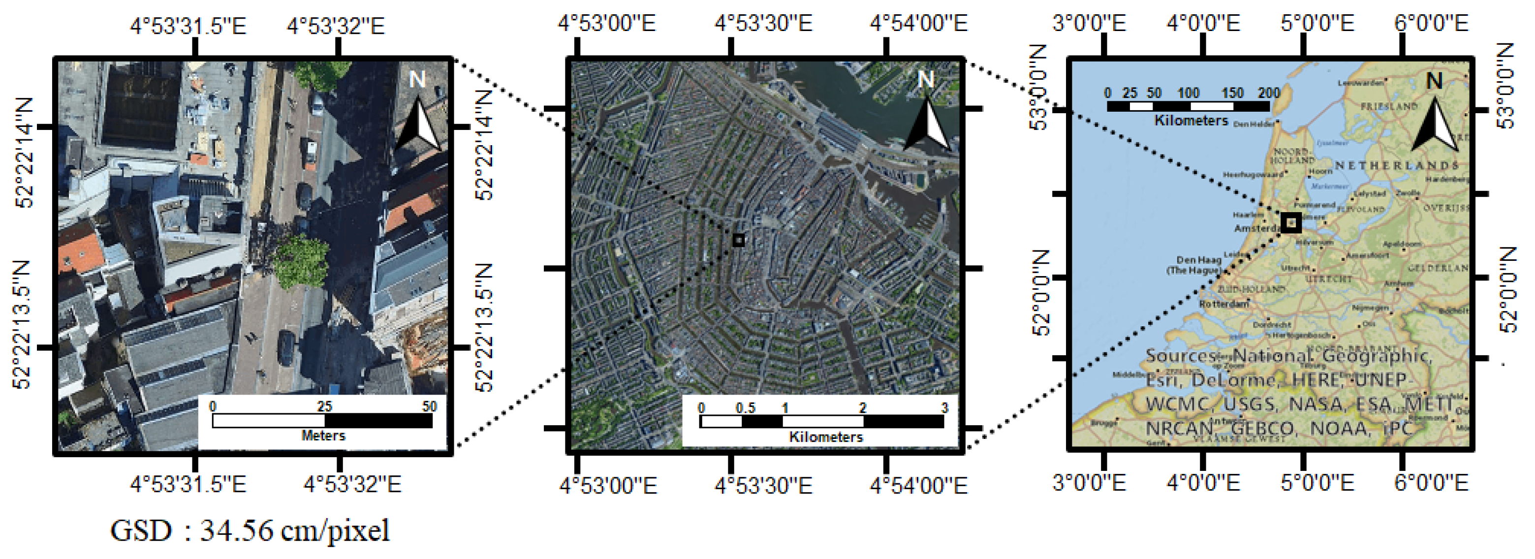
Object detection and semantic segmentation of the remote sensing image assume a fixed GSD. Some of the remote sensing image segmentation methods [3] use aerial datasets with a GSD value range of 5.0∼11.1 cm. However, they resize images to have similar GSD values by using the known GSD value of each dataset. As a result, the GSD range becomes 9.1∼11.1 cm with a variation of about 20%. Without knowing the GSD, their performance degrades unless they are resistent to large scale change. A sample of a remote sensing image with GSD is shown in Figure 1.

In real-world remote sensing cases, the GSD value is usually given from the metadata attached to or provided with the original image data. In this case, estimation of a GSD is not needed. Recently, however, there has been a growing number of applications [15,16,17,18,19,20] that deal with images obtained from online imagery providers such as Google Earth and Bing Maps that do not provide the real GSD for each screenshot. In such cases, it would be useful to estimate the GSD from the remote sensing image only.

If we have an input remote sensing image and there are georeferenced images for image matching whose pixel coordinates correspond to real-world coordinates, it is possible to estimate 6D global pose, position (including altitude which is related to GSD) and orientation in real-world coordinates [21,22]. Ground control points (GCP) also help with the estimation of position and direction [23]. In the case of training through the ground truth data, the altitude information can be estimated from learning the texture information of the remote sensing image, even without the georeferenced images [24].

In this paper, we present a regression approach for estimating the GSD from an input remote sensing image based on a convolutional neural network (CNN) without further information such as GCP, GPS or georeferenced images. We propose a regression tree CNN which consists of feature extraction CNN and a binomial tree layer. The feature extraction CNN first extracts features from an input image and then the binomial tree layer predicts the GSD value based on coarse scale classification and finer scale regression of the extracted features. The GSD value is predicted by first classifying the features to compute the target range or the coarse scale and then regressing the relative position or the finer scale within the target range. The prediction based on the coarse scale classification and the finer scale regression become possible by representing the GSD value as a floating-point number with the exponent and mantissa. When we combine the classification and regression, a classification error with the incorrect target range yields a large error on the final prediction, but some classification errors can be compensated for with our regression tree CNN architecture.

Our contributions are as follows: First, to the best of our knowledge, this paper is the first attempt to estimate the GSD for a remote sensing image based on neural networks. Second, the key part of the proposed network is the binomial tree layer, which improves regression by combining the classification and regression based on the floating-point representation. Our approach results in a reduction of 10.39% to 7.76% in relative errors compared to the direct estimation of GSD with a baseline network, which consists of a feature extraction CNN and two convolution layers.

2. Datasets

We first introduce eight public datasets, each of which contains images with a fixed single GSD value.

Table 1. Remote sensing image datasets with fixed GSDs.

Name	GSD	Image Size	Number of Images	Number of Pixels
ISPRS Potsdam [25]	5 cm	6000	38	1.37 G
VEDAI [26]	12.5 cm	1024	1267	1.33 G
Google Earth aerial [27]	15 cm	variable	variable	variable
UC Merced [28]	30 cm	256	2100	137.55 M
Digital Globe [29]	50 cm	1100∼8192	45	2.11 G
SkySat [30]	80 cm	1239∼3065	69	0.26 G
Massachusetts Roads [31]	100 cm	1024	1171	2.28 G
WiDS Datathon 2019 [32]	300 cm	256	21778	1.43 G

summarizes the eight datasets: ISPRS Potsdam [25], VEDAI [26], Google Earth aerial [27], UC Merced [28], Digital Globe [29], SkySat [30], Massachusetts Roads [31] and WiDS Datathon 2019 [32]. Each dataset consists of aerial or satellite images.

Datasets for remote sensing image scene classification, such as WHU-RS19 [15], RSCNN7 [16], AID [17], RSI-CB [18], NWPU-RESISC45 [19] and PatternNet [20], provide multiple GSDs. While each dataset contains images having different GSD values, the images with different GSD values are obtained by rescaling an image with a fixed GSD from Google Earth, Bing Maps or Google Maps.

We generate two types of datasets for our experiments: Dataset 1 is obtained from Google Earth aerial imagery in a similar way to the remote sensing image scene classification datasets mentioned above. On the other hand, dataset 2 is composed of images from the eight public datasets in Table 1.

2.1. Dataset 1: Rescaled Single Dataset (Google Earth)

The rescaled single dataset was created by rescaling the images acquired from aerial images in Google Earth. Since the Google Earth aerial images have a minimum GSD of 15 cm, the minimum GSD of dataset 1 was also set to 15 cm. Note that the images with a GSD smaller than 15 cm were not generated due to image blur. The maximum GSD was set to 480 cm, which equals 32 times 15 cm.

For Google Earth aerial images, the original GSDs without rescaling are 15 cm, 30 cm, 60 cm or more depending on the location. However, in order to utilize the images with the lowest GSD of 15 cm, we use the images from the 40 cities included in RoadTracer [4] as sampling locations. It appears that the images of these 40 cities were taken in consideration of various sensor environments and perspectives. In order to further diversify images, we use the most recently taken aerial images as well as aerial images taken at different times. We also rotate the images 0∼360 degrees and flip them to augment the data.

We generated two types of dataset 1, on a linear GSD scale and a log GSD scale, separately. For the dataset on the linear GSD scale, the images were generated to have uniform distribution over GSD values between 15 and 480 cm. For the dataset on the log GSD scale, we specify a real number x between 0 and 5 and use $15\times 2^x$ to extract the GSD values between 15 and 480. In this case, there are more samples with small GSDs and a smaller number of samples with large GSDs, but it has a uniform distribution on the log scale. Once the GSD value is determined, we obtain a 256 × 256 image at an arbitrary position within the area of 100 km${}^2$ for each city. We generate a total 50,000 images from 25 cities for training and 30,000 images from the remaining 15 cities for testing.

2.2. Dataset 2: Mixed Dataset

We constructed an additional dataset by mixing 8 datasets with different GSDs in Table 1. We need these datasets because if the images with different values of GSD are obtained by rescaling the images with one fixed original GSD, as in dataset 1, the network could simply learn the rescaling ratio without actually learning the GSD. To verify that the GSD prediction network does not simply output the rescaling ratio, we constructed a new dataset by mixing several datasets with different GSDs.

We built dataset 2 with 8 fixed GSD values from eight public datasets without rescaling. The size of the image was 256 × 256. We extracted 10,000 training images and 6000 test images for each dataset, with no overlap between training images and test images, resulting in a total of 80,000 training images and 48,000 test images.

3. Proposed Approach

In this section, we describe our deep learning regression approach to predicting the GSD value for a given remote sensing image. First, we explain why the predicted GSD value is represented by a floating-point number representation, after which we propose a regression tree CNN.

3.1. Floating-Point Regression of GSD

Our problem is to estimate the GSD value of an input remote sensing image using a CNN which is trained in a mini-batch. To train the CNN for regression, a loss function can be defined as absolute loss:

$$L_a=\sum _n\left|y_n-{\widehat{y}}_n\right|,$$

(1)

where $y_n$ is the ground truth GSD of n-th image in the mini-batch with N samples, and ${\widehat{y}}_n$ is the predicted GSD value. In this paper, we denote the variable without hat as the ground truth value and the variable with hat as the predicted value.

The absolute loss is actually the sum of the absolute errors. However, the absolute error of 3 cm with the true GSD value of 15 cm corresponding to a relative error of 20% could be considered to be worse than the absolute error of 3 cm with the true GSD value of 300 cm corresponding to a relative error of 1%. Thus, it is more reasonable to use the relative errors of 20% and 1%, not the absolute error of 3 cm. Relative error makes sense for GSD since it is measured on a ratio scale which has a true meaningful zero [33]. For example, on the Celsius temperature scale, the value 2 °C is not the true double of 1 °C, and relative error is meaningless because 0 °C is not the true meaningful zero. However, on the Kelvin temperature scale, 2 °K is the true double of 1 °K, and relative error is meaningful because 0 °K is the true meaningful zero, or absolute zero. In GSD, 0 cm is the true meaningful zero, and thus the relative error is a meaningful value. Hence we use the loss function that reflects the relative error. Intuitively, the loss function could be as follows:

$$L_r=\sum _n|\frac{y_n-{\widehat{y}}_n}{y_n}|=\sum _n\left|1-\frac{{\widehat{y}}_n}{y_n}\right|,$$

(2)

which is the sum of the relative errors.

We constructed a baseline network consisting of a feature extraction CNN and two convolution layers of 64 channels/1 channel that outputs the real value of GSD. As a training loss for the baseline network, we experimentally compared the relative loss Equation (2) with the absolute loss Equation (1) and obtained similar performance. The simple use of the relative loss Equation (2) as a loss function does not seem to yield a satisfactory result, and thus we formulate an alternative loss function, resulting in a floating-point representation of a GSD value and its implementation using a binomial tree layer.

The relative error is related to the logarithmic error, which is the difference on a log scale [34]:

$${\log }_2\left({\widehat{y}}_n\right)-{\log }_2\left(y_n\right)={\log }_2\left(\frac{{\widehat{y}}_n}{y_n}\right)={\log }_2\left(\frac{y_n-y_n+{\widehat{y}}_n}{y_n}\right)={\log }_2\left(1+\frac{{\widehat{y}}_n-y_n}{y_n}\right).$$

(3)

Using a Taylor series, $ln(1+x)\approx x$ with sufficiently small x, Equation (3) becomes:

$${\log }_2\left({\widehat{y}}_n\right)-{\log }_2\left(y_n\right)={\log }_2\left(1+\frac{{\widehat{y}}_n-y_n}{y_n}\right)\approx {\log }_2\left(e\right)\times \left(\frac{{\widehat{y}}_n-y_n}{y_n}\right).$$

(4)

Thus, the use of the logarithmic error as a loss reflects the relative error when training the network for the GSD prediction. Suppose GSD $y_n$ is expressed as an exponential form using an exponent with the real value $r_n$:

$$y_n=2^{lo{g}_2\left(y_n\right)}=2^{r_n}.$$

(5)

We decompose the real value exponent $r_n$ into the integer part $e_n$ and decimal part $d_n$, i.e., it is expressed as a floating-point representation with the real value mantissa of $m_n$ and the integer exponent of $e_n$:

$$y_n=2^{lo{g}_2\left(y_n\right)}=2^{r_n}=2^{e_n+d_n}=2^{d_n}\times 2^{e_n}=m_n\times 2^{e_n}.$$

(6)

The logarithmic loss using Equation (6) then becomes:

$${\log }_2\left({\widehat{y}}_n\right)-{\log }_2\left(y_n\right)=({\log }_2\left({\widehat{m}}_n\right)+{\widehat{e}}_n)-({\log }_2\left(m_n\right)+e_n)=({\widehat{e}}_n-e_n)+{\log }_2\left(\frac{{\widehat{m}}_n}{m_n}\right),$$

(7)

where the first term $({\widehat{e}}_n-e_n)$ represents the difference between the integer exponents, and the second term ${\log }_2({\widehat{m}}_n/m_n)$ represents the log ratio of the real value mantissas.

To properly associate the resulting value of the GSDs with the floating-point representation, we divide the target range of the GSDs into several segments/classes and determine the relative position within the segment. The segment is determined by coarse classification, and the relative position is computed by finer scale regression. Suppose the target range of 15∼480 cm. If 15∼480 cm is equally divided on the log scale, the five segments correspond to 15∼30 cm, 30∼60 cm, 60∼120 cm, 120∼240 cm and 240∼480 cm, which we call the log GSD scale classes. The corresponding reference value for each class is defined as 20 cm, 40 cm, 80 cm, 160 cm and 320 cm, respectively. For example, the value 50 cm is represented as the second class (log, 30∼60 cm, 40 cm) and the relative position of ×1.25 from its reference value 40 cm. Thus, the GSD value $y_n$ can be obtained from the floating-point representation:

$$y_n=20m_n{2}^{e_n},$$

(8)

where $e_n$ is the integer exponent ($e_n\in \{0,1,2,3,4\}$) corresponding to its class, and $m_n$ is the real number mantissa within the range of 0.75∼1.5. The constant 20 is used to properly represent the target range of each class by using the mantissa values of 0.75∼1.5.

Regarding our use of the log GSD scale classes defined above, we suppose the linear GSD scale classes that are defined by dividing the GSD range of 15∼480 cm into equal size segments of 15∼108 cm, 108∼201 cm, 201∼294 cm, 294∼387 cm and 387∼480 cm. The relative position is determined by the difference from a reference value. For example, if the reference value of 15∼108 cm is defined as 61.5 cm, 50 cm is represented by the first class (linear, 15∼108 cm) and the relative position of −11.5. The relative position divided by the interval value of 93 is expressed as a real value $m_n$ between −0.5 and 0.5. Additionally, defining $e_n$ as the integer class index ($e_n\in \{0,1,2,3,4\}$), the GSD value $y_n$ for the linear GSD scale classes is represented as follows:

$$y_n=(61.5+93e_n)+93m_n.$$

(9)

We expect that the log GSD scale classes improve the GSD prediction compared to the linear GSD scale classes since the log GSD classes better reflect the relative error through the logarithmic loss, as shown in Equation (7).

In this paper, we implement the first term in Equation (7) (the difference between the integer exponents) as a classification by using the cross entropy and then implement the second term in Equation (7) (the log ratio of the real value mantissas) as a regression by using the absolute loss, respectively, as follows:

$$L_y=\sum _n\sum _c{p}_{n,c}\log {\widehat{p}}_{n,c}+\lambda \sum _n\left|m_n-{\widehat{m}}_n\right|=L_e+\lambda L_m,$$

(10)

where $p_{n,c}$ represents the probability of the c-th class (corresponding to its appropriate exponent) of the n-th image in a mini-batch. The collection of $p_{n,c}$ is represented as a vector ${\mathit{p}}_n$ where $p_{n,c}$ is the c-th channel of the vector ${\mathit{p}}_n$. The ground truth ${\mathit{p}}_n$ is a one-hot vector representing the class of the image n where the one-hot vector is defined as a vector with all zero elements except a single one used to uniquely identify the class. For example, if the exponent $e_n$ is k, the class index is considered to be k, and thus $p_{n,k}$ becomes 1 and the others $p_{n,l}(l\ne k)$ are 0. Letting $m_n$ be the mantissa of the GSD for image n, ${\widehat{\mathit{p}}}_n$ and ${\widehat{m}}_n$ are then computed from the CNN, and ${\widehat{e}}_n$ is obtained from the arg-max of ${\widehat{p}}_{n,c}$ over c, resulting in ${\widehat{y}}_n$ using Equation (6).

We initially considered a simple multi-output network for exponent and mantissa prediction. If the mantissa range is limited to 0.75 to 1.5, only one pair of values for the exponent and the mantissa is associated with a specific GSD value. For example, if the GSD of an input remote sensing image is 36 cm, it corresponds to the second class (log, 30∼60 cm, 40 cm) and a mantissa of 0.9. However, when the classification error of one occurs with the same predicted mantissa value of 0.9, the predicted class becomes the first (log, 15∼30 cm, 20 cm) or third (log, 60∼120 cm, 80 cm), resulting in an incorrect GSD value of 18 cm or 72 cm. In order to compensate for this, we tried to train the adjusted ground truth mantissa value when the classification error occurs. For example, if the class becomes 1, the mantissa should be 1.8. However, the multiple pairs representing the same GSD value cause the problem of a one-to-many correspondence, which requires outputting multiple different pairs of values of the exponent and mantissa for the same input image. Our regression tree CNN allows the one-to-many correspondence, reducing the error caused by the classification by one, as described below.

3.2. Regression Tree CNN

Figure 2 shows our proposed regression tree CNN consisting of a feature extraction CNN and a binomial tree layer, the output of which is used to form a floating-point representation of the GSD value for a given input image. Features are first extracted by the CNN from an input image and are then input to the binomial tree layer. By combining the exponent and mantissa from the binomial tree, we obtain the GSD prediction.

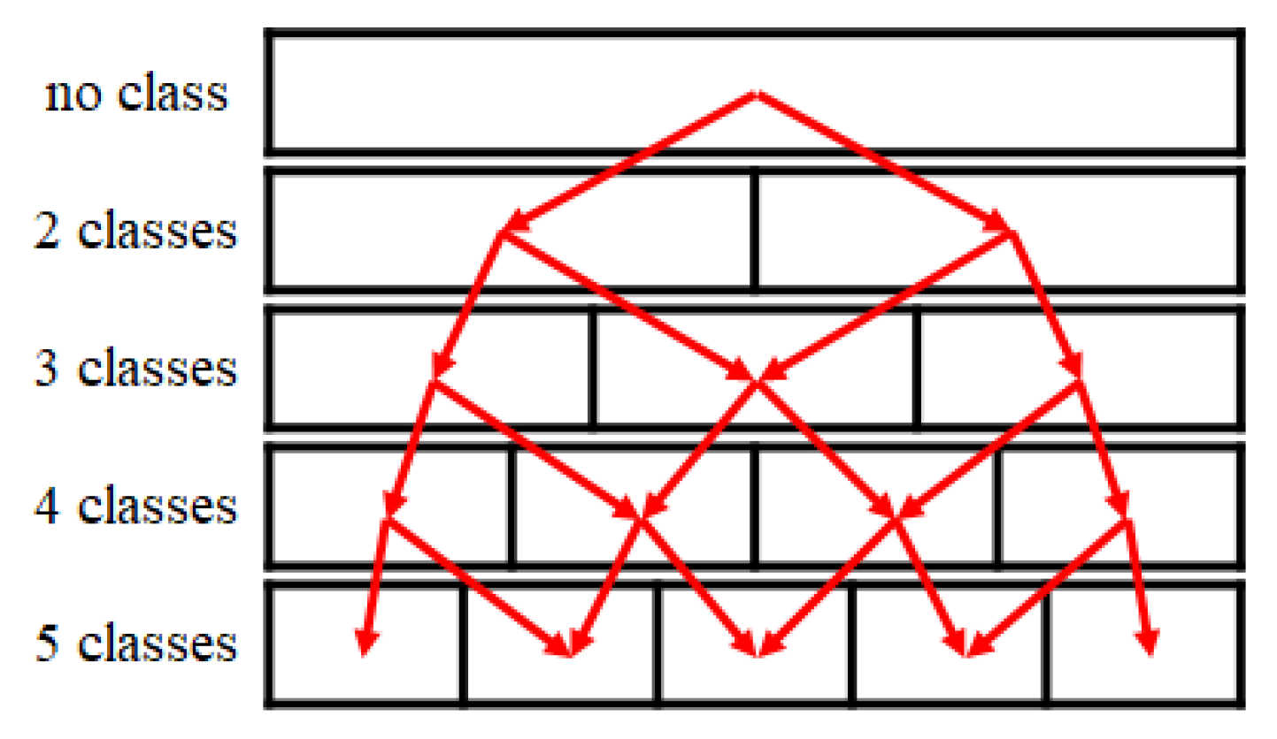
To design a network that performs both classification and regression simultaneously, we employ the vector representation of the CapsNet [35] with some modification. We estimate an output vector which is used to select the class (or exponent) and to estimate the mantissa. To improve the classification at the class boundary, we successively refine the classification with the binomial tree structure, as shown in Figure 3. Because the child-level class boundaries reside within the parent-level classes from the root to its leaves, the information related to the class boundary can be better delivered, improving both the classification and regression. We call the whole structure a binomial tree layer.

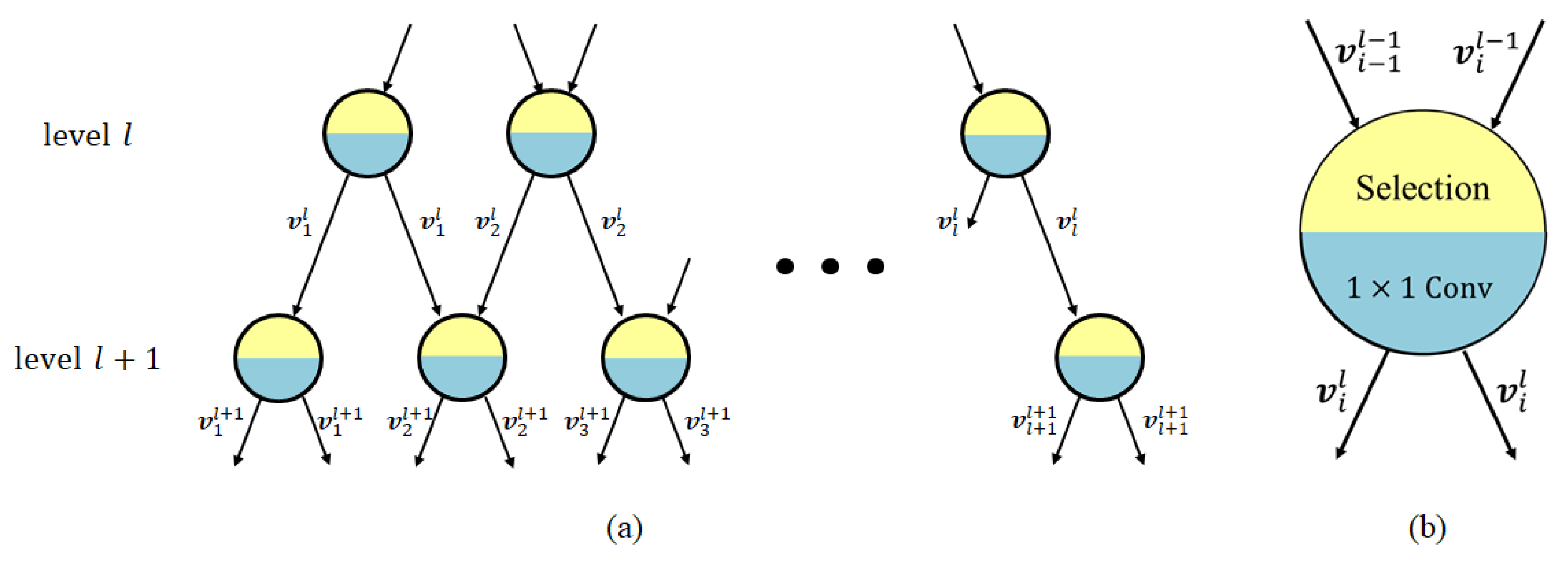
The root node contains the feature map of the last convolution layer of the feature extraction CNN. The number of nodes grows one by one as the tree becomes deeper, as shown in Figure 4. Of the two vectors associated with the two parent nodes, only the one with the larger length is transmitted to the next level. Node selection in the binomial tree layer is performed using the following equation:

$${\mathit{v}}_i^l={conv}_i^l\left({\mathit{v}}_{\widehat{k}}^{l-1}\right)\mathrm{where}\widehat{k}=\underset{k\in \{i-1,i\}}{argmax}∥{\mathit{v}}_k^{l-1}∥,$$

(11)

where ${\mathit{v}}_i^l$ and conv${}_i^l$ denote the feature vector and the pointwise convolution of the i-th node at level l, respectively. The feature vector with the larger length is selected, and a pointwise convolution is performed.

To train the pointwise convolution for each node, the local classification among l classes is performed using the length of the l vectors at level l. For example, the local class border is defined by $15\times {(480/15)}^{i/l},i=0,1,...,l$. At level 3, we perform a classification of three classes with the ranges of 15.00∼47.62, 47.62∼151.19 and 151.19∼480.00.

In the leaf nodes, we compute the exponent and mantissa to estimate the GSD value. The V-dimensional vector with the maximum $L_2$ norm among C vectors is selected, and the class or the integer exponent is determined by the leaf node containing the largest vector. The values of C = 5 and V = 16 are used. We then normalize the selected vector and perform two pointwise convolutions of 64 channels/1 channel to estimate the mantissa. The whole architecture of the proposed network is shown in Figure 2.

If an error occurs during the classification, especially when the classification differs by one from the correct vector, our binomial tree layers can reduce the resulting GSD prediction error by adaptively adjusting the mantissa value for the incorrectly selected vector. The incorrectly selected vector is trained to output the adjusted mantissa value, which is different from the mantissa value for the correctly selected vector. Due to the one-to-many correspondence training, the final prediction becomes correct despite the classification error. Because most of the classification errors had a size of 1 in the experiments, we only consider the class errors of size 1 by training the additional two pairs of the class vector k− 1 and k + 1 and their respective mantissa values for the correct class vector k.

During backpropagation, the weight update is affected by the selected leaf node and the corresponding path. In Figure 2, the weights of the nodes on the path are updated by $L_e$ and $L_m$ in Equation (10), and the weights of the other nodes are updated by only $L_e$ in Equation (10). However, considering the mini-batch size of N, the corresponding N paths are trained simultaneously in the mini-batch. For each path leading to a correct class vector, we augment 10% of the data with the simulated classification errors of size 1 and the corresponding adjusted mantissa value during training.

As a feature extraction CNN, 1.0 MobileNet-224 [36] and ResNet-101 [37] are used. The number of channels of the last feature maps from the feature extraction CNN is 1024 for MobileNet and 2048 for ResNet. We excluded the global average pooling or the fully connected layers of the original networks.

While the tree structure was also used in option pricing [38], Tree-CNN [39] and the classification and regression tree (CART) [40], our regression tree CNN estimates the GSD by computing the exponent (classification), calculating the mantissa (regression) and then combining them.

4. Experimental Results

We implemented the proposed network using TensorFlow on a single Titan X GPU. We adopted MobileNet as the feature extraction CNN for all experiments due to its simplicity, although better results were consistently obtained by using ResNet-101. For comparison, we also implemented the baseline network described earlier. For both the proposed and baseline networks, denoting the height and width of the final output by the same M, the value of M is set to 8 for the input image of 256 × 256. The $M^2$ values are averaged to obtain the final GSD value.

To evaluate the performance of our approach for estimating the value of GSD for a given image, we used the datasets of the linear GSD scale dataset 1, the log GSD scale dataset 1 and dataset 2 described in Section 2.

As mentioned in Section 2.1, since dataset 1 was generated by rescaling Google Earth aerial images with a single fixed original GSD of 15 cm, the training with dataset 1 could be suspected of making the proposed regression tree CNN learn the rescaling ratio rather than the GSD. Thus, we also performed experiments with dataset 2, which contains remote sensing images with different original GSDs. However, since each image in dataset 2 can have only one of the eight fixed values of GSD, we expect to easily learn the GSD of each image in dataset 2. Thus, dataset 2 is only used supplementarily to show that our regression tree CNN does not simply learn the rescaling ratio but learns the GSD value as intended. We conducted most of our experiments with dataset 1.

To demonstrate the applicability of the proposed GSD prediction, we also performed experiments for RoadTracer with the aerial images with various GSDs obtained from Google Maps.

4.1. Training Details

For dataset 1, we used the image sizes 128, 256 and 512. There were 50,000 training images and 30,000 test images for each of log GSD scale dataset 1 and linear GSD scale dataset 1. As described before, the range of GSDs was set to 15∼480 cm with five classes starting from 15 cm. For dataset 2, we used an image size of 256. Dataset 2 was built from the eight public datasets without image rescaling. There were 80,000 training images and 48,000 test images. The range of GSDs was set to 5∼320 cm with six classes and starting from 5 cm.

The batch size was set to 32, and Adam [41] was used for the optimization. The initial learning rate was set to ${10}^{-4}$ with a decay of 0.1. The weights were initialized with He initialization [42]. We used $L_2$ regularization for the weights. The experiments were performed for 32 epochs, and the learning rate decay was applied to the 16th and 24th epochs. The example loss plot over training epochs for the proposed method with the log GSD scale dataset 1 is shown in Figure 5.

We repeated the experiments five times. Each experiment was randomized by using a random set of initial weights and a randomly selected 90% of the training data. To measure the stability of each experiment, the standard deviation of the experiment was utilized together with its mean.

4.2. Learning GSD Prediction

To see how the GSD prediction is learned, we observed the feature map of the last convolution layer of the feature extraction CNN, as shown in Figure 6. Using the Google Earth aerial image of Amsterdam from dataset 1 (rescaled single dataset), we sampled 500 images which had GSDs of 15∼480 cm, with a resize ratio of $({(480/15)}^{1/500}-1)\times 100=0.696\%$. The GSDs of the images are 15.00, 15.10, ..., 476.68 and 480.00.

For a 256 × 256 input image, the feature extraction CNN output an 8 × 8 × 1024 feature map, which was averaged horizontally and vertically to a 1024-channel map. For visualization purposes, we stacked 1024-channel maps from 500 images, resulting in an image of 500 × 1024 in Figure 6b,c. The top row corresponds to the feature map of an input image with 15 cm, and the bottom row represents the feature map of 480 cm. Then, we sorted the columns of the stacked feature map so that the columns whose upper part values are larger go to the left side and the columns whose lower part values are larger go to the right side.

Figure 6b shows the stacked feature map of the ImageNet pre-trained network, whereas Figure 6c represents the stacked feature map of our GSD-trained baseline network. Figure 6b does not show a pattern depending on the different values of GSD whereas Figure 6c presents a clear pattern that certain columns have large values responding to the GSD values. We observed that the channels show a reasonable amount of correlation with GSD values from 15 cm to 480 cm. Figure 6c suggests that the GSD values could be divided into several coarse scale classes and then represented by the finer scale relative position from the corresponding coarse scale class.

4.3. Performance Analysis with Dataset 1 (Rescaled Single Dataset)

We conducted our experiments with dataset 1 as follows: We first compared the GSD prediction error of our approach with the baseline method, as shown in in

Table 2. Comparison of GSD prediction errors and the number of parameters for the log GSD scale dataset 1.

Method	Number of Parameters	Error (%)
Baseline ($L_a$)	3.19 M	10.41 ± 0.25
Baseline ($L_r$)	3.19 M	10.39 ± 0.27
Baseline ($L_r$, Additional layers)	3.20 M	10.17 ± 0.38
Proposed (MobileNet)	3.22 M	7.76 ± 0.17
Proposed (ResNet)	42.52 M	7.02 ± 0.20

. We also investigated the effect of various factors on performance, such as the linear/log GSD scale (

Table 3. Comparison of GSD prediction errors for the linear and the log GSD scale dataset 1.

Error (%)		Training Dataset (Linear)	Training Dataset (Log)
Baseline	Test dataset (Linear)	10.91 ± 0.38	10.53 ± 0.26
	Test dataset (Log)	19.20 ± 1.43	10.39 ± 0.27
Proposed (linear GSD scale classes)	Test dataset (Linear)	8.97 ± 0.30	8.90 ± 0.12
	Test dataset (Log)	11.90 ± 1.02	8.87 ± 0.16
Proposed (log GSD scale classes)	Test dataset (Linear)	8.31 ± 0.17	8.11 ± 0.11
	Test dataset (Log)	10.37 ± 0.58	7.76 ± 0.17

), the cost combination (

Table 4. GSD prediction errors for cost combination with the log GSD scale dataset 1.

${\mathit{L}}_{\mathit{r}}$	${\mathit{L}}_{\mathit{e}}$	${\mathit{L}}_{\mathit{m}}$	Error (%)
o			510.44 ± 7.95
o		o	252.37 ± 90.66
o	o		8.24 ± 0.11
o	o	o	8.21 ± 0.15
	o	o	7.76 ± 0.17

), the image size (

Table 5. GSD prediction errors according to the training and test image sizes with the log GSD scale dataset 1.

Error (%)	Training-128	Training-256	Training-512
Test-128	15.02 ± 0.33	18.89 ± 0.96	14.25 ± 0.34
Test-256	13.17 ± 2.01	7.76 ± 0.17	7.76 ± 0.06
Test-512	13.50 ± 3.14	5.35 ± 0.13	5.29 ± 0.08

) and the value of $\lambda$ (

Table 6. GSD prediction performance for the different values of weight $\lambda$ with the log GSD scale dataset 1.

$\mathit{\lambda }$	0.01	0.1	1.0	10.0	100.0
Classification accuracy (%)	94.12 ± 0.10	93.98 ± 0.05	94.17 ± 0.01	93.66 ± 0.20	90.43 ± 0.12
Mantissa error (×100)	9.47 ± 0.13	6.81 ± 0.05	5.10 ± 0.04	4.23 ± 0.03	2.99 ± 0.09
GSD prediction error (%)	10.76 ± 0.12	9.30 ± 0.01	7.96 ± 0.16	7.76 ± 0.17	9.71 ± 0.36

). We evaluated our proposed method with the loss in Equation (10), the input image size of 256 and $\lambda$ of 10 unless otherwise stated.

4.3.1. Baseline Method vs. the Proposed Method

Table 2 shows a comparison of the resulting relative errors of GSD prediction obtained by our proposed network and the baseline network using the log GSD scale dataset 1. Our network yields the relative error of 7.76% compared to 10.39% when using the baseline network, which is a relative reduction of 25.31%. We see that the use of relative loss in Equation (2) does not improve the performance compared to the absolute loss in Equation (1) for the baseline network. The performance of the proposed network was better than that of the baseline network with the additional pointwise convolution layer of 16-16-16-16-16-64 channels, which can be considered equivalent to the proposed regression tree CNN with a single fixed path. This implies that the superiority of the proposed network is due to the addition of the binomial tree layer. The use of ResNet rather than MobileNet slightly reduced the relative error by 0.74%. We also see that the number of parameters needed to implement the binomial tree layer is 0.03 M (= 3.22 M – 3.19 M), which is only about 1% of 3.22 M, but this layer significantly reduces the GSD prediction error.

4.3.2. Linear GSD Scale vs. Log GSD Scale

Table 3 shows a comparison of the resulting relative errors of GSD prediction obtained by our proposed network and the baseline network using the linear GSD scale dataset 1 and the log GSD scale dataset 1 as the training and test datasets in four different combinations. The baseline network was trained by using the relative cost in Equation (2).

In Table 3 we can see that the proposed network yields GSD prediction errors lower than the baseline network under four different dataset conditions. We also observe that the training with log GSD scale dataset 1 reduces the GSD prediction errors regardless of the networks used and the GSD scales of the test datasets. The use of the log GSD scale classes lowers the GSD prediction errors compared with the linear GSD scale classes. This is because the use of the log GSD scale classes during training minimizes the logarithmic error which corresponds to the relative error, as mentioned in Section 3.1, whereas the linear GSD scale classes only utilize the linear combination of classification and regression in Equation (9) and thus do not appropriately reflect the relative error. Thus, we can achieve better performance with the proposed network when it is trained on log GSD scale dataset 1 based on the log GSD scale classes.

We performed additional experiments on the proposed network with log GSD scale dataset 1 (for training and testing) based on the log GSD scale classes, as shown in Table 4, Table 5 and Table 6 and Figure 7.

4.3.3. Cost Combination

Table 4 shows the performance variation of the proposed network, the regression tree CNN, with respect to the cost combinations of $L_r$, $L_e$ and $L_m$ used in training. As described earlier, $L_r$, $L_e$ and $L_m$ affect the actual value of GSD, the target range (class or exponent) and the mantissa or the relative position in the class, respectively. We can see that the use of $L_e$ greatly reduces the GSD prediction errors and the additional use of $L_m$ further reduces the errors. The best performance is achieved by using both $L_e$ and $L_m$ in Equation (10) in training. If we additionally use $L_r$ with $L_e$ and $L_m$, three terms should simultaneously converge to a minimum in ideal case. However, the network could be trained in a way that locally minimizes $L_r$ at the larger values of $L_e$ and $L_m$, when $L_r$ is dominant. This could create an unsatisfactory local minimum, resulting in the increased GSD prediction error.

4.3.4. Image Size

Table 5 shows the GSD prediction errors resulting from the proposed network according to the sizes of the training and test images. The value of GSD ranges from 15 cm to 480 cm, as before. We see that for the same size of training image, the larger the size of the test image is the smaller the GSD prediction error is since the network seems to extract more cues for GSD from the larger area. We also observe that the appropriate size of the training images is 256.

4.3.5. Value of Weight $\lambda$

Weight $\lambda$ in Equation (10) controls the balance between the classification and the regression. Table 6 shows the classification accuracy (exponent accuracy), regression error (mantissa error) and the resulting GSD prediction error. There is a tradeoff between the classification accuracy and the mantissa error; it shows the best GSD estimation performance when $\lambda$ is 10.0, which was used in our experiments.

4.3.6. GSD Prediction Examples

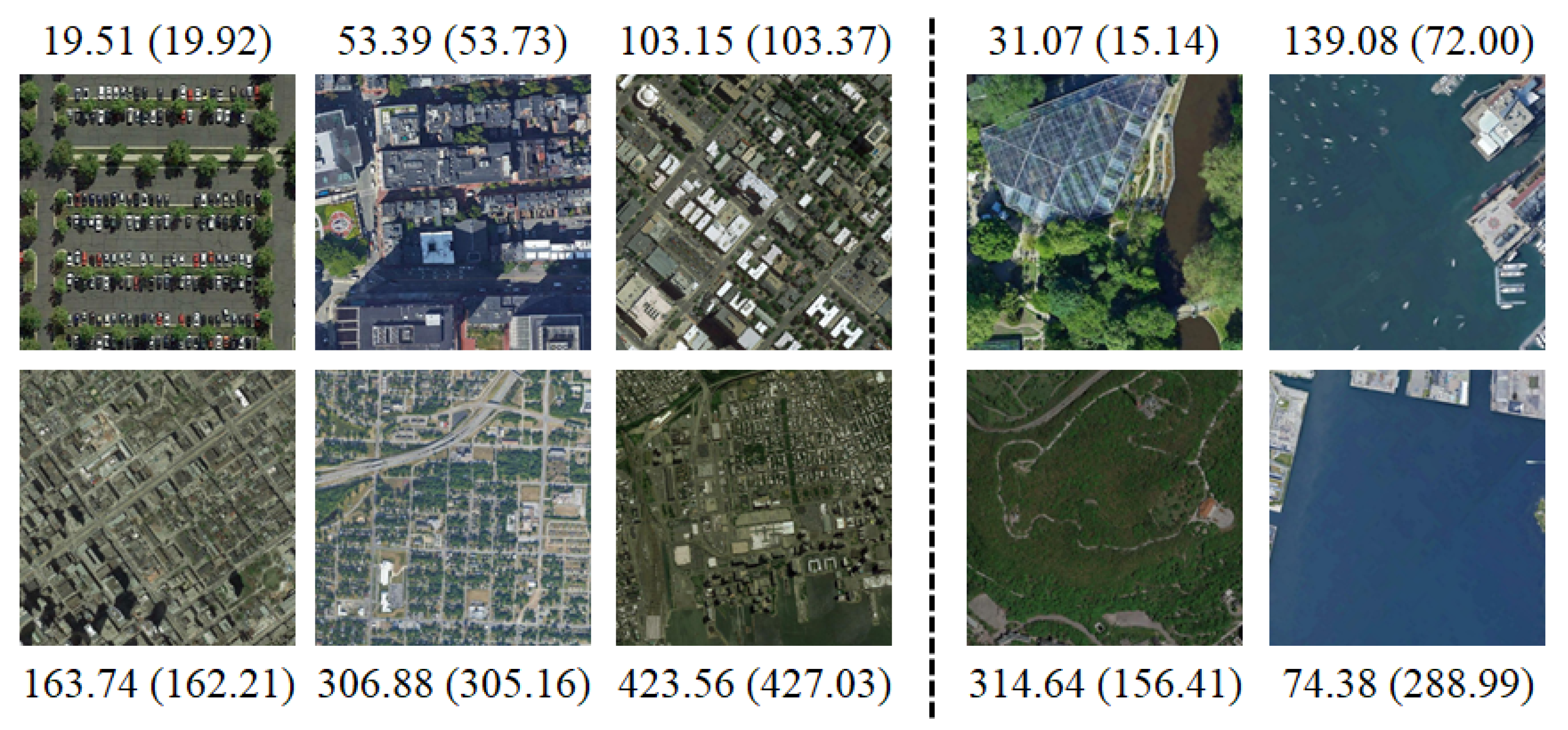
Figure 7 shows the GSD prediction results of log GSD scale dataset 1 (rescaled single dataset) with an image size of 512. We show the 6 images with a GSD prediction error lower than 5% and the four images with a GSD prediction error larger than 40%. We see that an input image with standardized objects such as cars, buildings and roads seems to yield good GSD prediction whereas unstructured objects such as water, trees or other natural objects are not beneficial for GSD prediction. When the GSD value is small, the prediction results are sometimes not satisfactory if the size of an object is too large compared to the size of its image.

4.4. Experiments with Dataset 2 (Mixed Dataset)

We conducted experiments on the mixed dataset with the baseline network and the proposed regression tree CNN, as shown in

Table 7. GSD prediction errors of the mixed dataset experiment.

	Baseline	Proposed
Error (%)	1.88 ± 0.26	0.06 ± 0.01

. Since the range of GSD (5∼320) is different from the case of dataset 1, training and testing were performed based on the six log GSD scale classes of 5∼10, 10∼20, 20∼40, 40∼80, 80∼160 and 160∼320 where the depth of the binomial tree and number of leaf nodes are set to 6. As mentioned in Section 4.3.4, since the optimal training image size for GSD prediction seems to be 256, we also used an image size of 256 for dataset 2.

For the mixed dataset without image rescaling, the networks simply need to learn to recognize 8 integers of GSD values where each integer value is associated with the corresponding dataset, which results in significantly lower GSD prediction errors, as shown in Table 7. We can also see that the proposed network yields the much lower error of 0.06% compared with 1.88% obtained from the baseline network because the proposed network needs to process only one or two datasets for each leaf node.

From the experiments with datasets 1 and 2, we can see that the proposed network does not simply learn the rescaling ratio but is capable of learning the GSD value. Figure 8 shows the GSD prediction results of the mixed dataset with the image size of 256. Since the GSD prediction error is too low, we could not find any bad prediction examples.

4.5. Application of Proposed Approach to RoadTracer

To illustrate the significance of our proposed approach, we conducted experiments to investigate if the predicted GSD value can improve the performance of other related methods, such as road detection and segmentation. Specifically, we performed experiments with RoadTracer [4]. We trained RoadTracer on the images of the fixed GSD value of 60 cm in the same way as in [4], but tested it on images with various GSD values ranging from 30 cm to 120 cm. We used 3 types of test images: (i) The original images with a fixed GSD of 60 cm; (ii) images with various GSDs ranging from 30 cm to 120 cm and (iii) the same images as the second type but resized to match their GSDs to 60 cm using our predicted GSD values from the proposed network trained on the log GSD scale dataset 1. Using the predicted GSDs of the second type images, the GSDs of the third type images became 56.07 cm∼63.67 cm.

RoadTracer differs from the semantic segmentation of a road in that the center pixel of an arbitrary road is given as input and RoadTracer uses the cropped 256 × 256 image centered on that pixel. As a result, the size of an input image can be arbitrary, although 8192 × 8192 images were used in [4]. RoadTracer finds the direction of a road from the center pixel and travels a fixed distance D = 12 m. After that, a small image centered on the moved location is cropped, and then the road graph is iteratively constructed. RoadTracer was only applied to the images with the fixed GSD of 60 cm, and there was no discussion of what happens when an image with different GSD values is used as input. In general, if the GSD of an image changes, the typical size of an object such as a building or car in the image changes too. Thus, RoadTracer is unlikely to cross a large road if the GSD of an image is quite smaller than the GSD on which it was trained, or it can skip some alleys if the GSD of an image is too large.

Figure 9 illustrates this phenomenon. For the first type of images, the road graphs were well extracted. For the third type of images, resized to match the predicted GSD of 60 cm, the results are similar to the first type images. However, for the second type of images, the results are not satisfactory. As shown in Figure 9a, if the image had a GSD value smaller than 60 cm, the width of the road in the image became larger, which made it difficult to track the multi-lane road at the intersection. On the other hand, as shown in Figure 9b, when the GSD value was larger than 60 cm, the width of the road became smaller, which made RoadTracer skip the narrow road. The RoadTracer experiments show that the predicted GSD greatly helps in the detection of roads.

5. Conclusions

In this paper, we have proposed a regression tree CNN for estimating GSD from a remote sensing image. The regression tree CNN consists of two parts, the feature extraction CNN and the binomial tree layer. The binomial tree layer is based on a floating-point representation to combine the classification and regression on the log GSD scale. The experiments demonstrate the feasibility of our approach, which shows an improvement of 25.31% in error rate over the baseline method. Our approach for predicting the GSD value is useful in itself and is applicable to applications using remote sensing images as input, including road detection and segmentation.

References

1. Isola, P.; Zhu, J.Y.; Zhou, T.; Efros, A.A. Image-to-image translation with conditional adversarial networks. In Proceedings of the Conference on Computer Vision and Pattern Recognition, Honolulu, HI, USA, 21–26 July 2017; pp. 5967–5976. [Google Scholar]
2. Audebert, N.; Le Saux, B.; Lefèvre, S. Segment-before-detect: Vehicle detection and classification structure through semantic segmentation of aerial images. Remote Sens. 2017, 9, 368. [Google Scholar] [CrossRef]
3. Kaiser, P.; Wegner, J.D.; Lucchi, A.; Jaggi, M.; Hofmann, T.; Schindler, K. Learning aerial image segmentation from online maps. IEEE Trans. Geosci. Remote Sens. 2017, 55, 6054–6068. [Google Scholar] [CrossRef]
4. Bastani, F.; He, S.; Abbar, S.; Alizadeh, M.; Balakrishnan, H.; Chawla, S.; Madden, S.; DeWitt, D. RoadTracer: Automatic extraction of road networks from aerial images. Comput. Vis. Pattern Recognit. 2018, 4720–4728. [Google Scholar] [CrossRef]
5. Al Rahhal, M.; Bazi, Y.; Abdullah, T.; Mekhalfi, M.; AlHichri, H.; Zuair, M. Learning a multi-branch neural network from multiple sources for knowledge adaptation in remote sensing imagery. Remote Sens. 2018, 10, 1890. [Google Scholar] [CrossRef]
6. Chen, Y.; Li, Y.; Jiao, L.; Peng, C.; Zhang, X.; Shang, R. Adversarial reconstruction-classification networks for polsar image classification. Remote Sens. 2019, 11, 415. [Google Scholar] [CrossRef]
7. Paoletti, M.; Haut, J.; Plaza, J.; Plaza, A. Deep&Dense convolutional neural network for hyperspectral image classification. Remote Sens. 2018, 10, 1454. [Google Scholar]
8. Li, Y.; Zhang, H.; Shen, Q. Spectral–spatial classification of hyperspectral imagery with 3D convolutional neural network. Remote Sens. 2017, 9, 67. [Google Scholar] [CrossRef]
9. Sellami, A.; Farah, M.; Farah, I.R.; Solaiman, B. Hyperspectral imagery classification based on semi-supervised 3-D deep neural network and adaptive band selection. Expert Syst. Appl. 2019, 129, 246–259. [Google Scholar] [CrossRef]
10. Altwaijry, H.; Trulls, E.; Hays, J.; Fua, P.; Belongie, S. Learning to match aerial images with deep attentive architectures. In Proceedings of the IEEE Conference on Computer Vision and Pattern Recognition, Las Vegas, NV, USA, 27–30 June 2016; pp. 3539–3547. [Google Scholar]
11. Duque, J.; Patino, J.; Betancourt, A. Exploring the potential of machine learning for automatic slum identification from VHR imagery. Remote Sens. 2017, 9, 895. [Google Scholar] [CrossRef]
12. So, B.; Nezin, C.; Kaimal, V.; Keene, S.; Collins, L.; Bradbury, K.; Malof, J.M. Estimating the electricity generation capacity of solar photovoltaic arrays using only color aerial imagery. In Proceedings of the IEEE International Geoscience and Remote Sensing Symposium (IGARSS), Fort Worth, TX, USA, 23–28 July 2017; pp. 1603–1606. [Google Scholar]
13. Zhu, X.X.; Tuia, D.; Mou, L.; Xia, G.S.; Zhang, L.; Xu, F.; Fraundorfer, F. Deep learning in remote sensing: A comprehensive review and list of resources. IEEE Geosci. Remote Sens. Mag. 2017, 5, 8–36. [Google Scholar] [CrossRef]
14. Ball, J.E.; Anderson, D.T.; Chan, C.S. Comprehensive survey of deep learning in remote sensing: Theories, tools, and challenges for the community. J. Appl. Remote Sens. 2017, 11, 042609. [Google Scholar] [CrossRef]
15. Yu, H.; Yang, W.; Xia, G.S.; Liu, G. A color-texture-structure descriptor for high-resolution satellite image classification. Remote Sens. 2016, 8, 259. [Google Scholar] [CrossRef]
16. Zou, Q.; Ni, L.; Zhang, T.; Wang, Q. Deep learning based feature selection for remote sensing scene classification. IEEE Geosci. Remote Sens. Lett. 2015, 12, 2321–2325. [Google Scholar] [CrossRef]
17. Xia, G.S.; Hu, J.; Hu, F.; Shi, B.; Bai, X.; Zhong, Y.; Zhang, L.; Lu, X. AID: A benchmark data set for performance evaluation of aerial scene classification. IEEE Trans. Geosci. Remote Sens. 2017, 55, 3965–3981. [Google Scholar] [CrossRef]
18. Li, H.; Tao, C.; Wu, Z.; Chen, J.; Gong, J.; Deng, M. RSI-CB: A large scale remote sensing image classification benchmark via crowdsource data. arXiv 2017, arXiv:1705.10450. [Google Scholar]
19. Cheng, G.; Han, J.; Lu, X. Remote sensing image scene classification: Benchmark and state of the art. Proc. IEEE 2017, 105, 1865–1883. [Google Scholar] [CrossRef]
20. Zhou, W.; Newsam, S.; Li, C.; Shao, Z. PatternNet: A benchmark dataset for performance evaluation of remote sensing image retrieval. ISPRS J. Photogramm. Remote Sens. 2018, 145, 197–209. [Google Scholar] [CrossRef] [Green Version]
21. Shetty, A.; Gao, G.X. UAV pose estimation using cross-view geolocalization with satellite imagery. arXiv 2018, arXiv:1809.05979. [Google Scholar]
22. Grelsson, B. Global Pose Estimation from Aerial Images: Registration with Elevation Models. Ph.D. Thesis, Linköpings Universitet, Linköping, Sweden, 2014. [Google Scholar]
23. Tjahjadi, M.E.; Agustina, F.D. Single image orientation of UAV’s imagery using orthogonal projection model. Int. Symp. Geoinf. 2017, 18–23. [Google Scholar]
24. Cherian, A.; Andersh, J.; Morellas, V.; Papanikolopoulos, N.; Mettler, B. Autonomous altitude estimation of a UAV using a single onboard camera. In Proceedings of the IEEE International Conference on Intelligent Robots and Systems, St. Louis, MO, USA, 10–15 October 2009; pp. 3900–3905. [Google Scholar]
25. Rottensteiner, F.; Sohn, G.; Jung, J.; Gerke, M.; Baillard, C.; Benitez, S.; Breitkopf, U. ISPRS Benchmark on Urban Classification and 3D Building Reconstruction. ISPRS Ann. Photogramm. Remote Sens. Spat. Inf. Sci. I-3 2012, 1, 293–298. [Google Scholar] [CrossRef]
26. Razakarivony, S.; Jurie, F. Vehicle detection in aerial imagery: A small target detection benchmark. J. Vis. Commun. Image Represent. 2016, 34, 187–203. [Google Scholar] [CrossRef]
27. Google Earth. Available online: https://www.google.com/earth/ (accessed on 25 June 2019).
28. Yang, Y.; Newsam, S. Bag-of-visual-words and spatial extensions for land-use classification. In Proceedings of the 18th SIGSPATIAL International Conference on Advances in Geographic Information Systems, San Jose, CA, USA, 2–5 November 2010; pp. 270–279. [Google Scholar]
29. Digital Globe Product Samples. Available online: https://www.digitalglobe.com/samples (accessed on 25 June 2019).
30. SkySat High Resolution Image Samples. Available online: https://info.planet.com/download-free-high-resolution-skysat-image-samples/ (accessed on 25 June 2019).
31. Mnih, V. Machine Learning for Aerial Image Labeling; University of Toronto: Toronto, ON, Canada, 2013. [Google Scholar]
32. WiDS Datathon 2019. Available online: https://www.kaggle.com/c/widsdatathon2019/data (accessed on 25 June 2019).
33. Michell, J. Quantitative science and the definition of measurement in psychology. Br. J. Psychol. 1997, 88, 355–383. [Google Scholar] [CrossRef]
34. King, R.F.; Phillips, D.L. The logarithmic error and Newton’s method for the square root. Commun. ACM 1969, 12, 87–88. [Google Scholar] [CrossRef]
35. Sabour, S.; Frosst, N.; Hinton, G.E. Dynamic routing between capsules. In Proceedings of the 31st International Conference on Neural Information Processing Systems, Long Beach, CA, USA, 4–9 December 2017. [Google Scholar]
36. Howard, A.G.; Zhu, M.; Chen, B.; Kalenichenko, D.; Wang, W.; Weyand, T.; Andreetto, M.; Adam, H. Mobilenets: Efficient convolutional neural networks for mobile vision applications. arXiv 2017, arXiv:1704.04861. [Google Scholar]
37. He, K.; Zhang, X.; Ren, S.; Sun, J. Identity mappings in deep residual networks. In Proceedings of the European Conference on Computer Vision, Amsterdam, The Netherlands, 8–16 October 2016; pp. 630–645. [Google Scholar]
38. Cox, J.C.; Ross, S.A.; Rubinstein, M. Option pricing: A simplified approach. J. Financ. Econ. 1979, 7, 229–263. [Google Scholar] [CrossRef]
39. Roy, D.; Panda, P.; Roy, K. Tree-CNN: A hierarchical deep convolutional neural network for incremental learning. arXiv 2018, arXiv:1802.05800. [Google Scholar] [CrossRef]
40. Breiman, L. Classification and regression trees. Routledge 2017. [Google Scholar] [CrossRef]
41. Kingma, D.P.; Ba, J. Adam: A method for stochastic optimization. arXiv 2014, arXiv:1412.6980. [Google Scholar]
42. He, K.; Zhang, X.; Ren, S.; Sun, J. Delving deep into rectifiers: Surpassing human-level performance on imagenet classification. In Proceedings of the IEEE International Conference on Computer Vision, Santiago, Chile, 11–18 December 2015; pp. 1026–1034. [Google Scholar]
Figure 1. A sample of a remote sensing image with ground sampling distance (GSD) that was obtained using Google Earth.
Remotesensing 11 02276 g001
Figure 2. The architecture of the regression tree convolutional neural network (CNN), which consists of the feature extraction CNN and the binomial tree layer. For the feature extraction CNN, we use MobileNet [36] (1024-D) or ResNet [37] (2048-D).
Remotesensing 11 02276 g002
Figure 3. Successive refinement of classification.
Remotesensing 11 02276 g003
Figure 4. Node selection in the binomial tree layer: (a) For vectors of l nodes at level l, we perform local classification of l classes using the vector length. Each vector information is transmitted to the appropriate nodes at the next level; (b) we select the vector with larger length and apply a 1×1 convolution.
Remotesensing 11 02276 g004
Figure 5. The example loss plot over training epochs of the proposed method with the log GSD scale dataset 1.
Remotesensing 11 02276 g005
Figure 6. Input images from a Google Earth aerial image of Amsterdam and their stacked feature maps of the last convolution layer of the feature extraction CNN. Each row represents a 1024-D feature map of an image having a specific GSD: (a) 500 sample images with a resize ratio of 0.696%; (b) ImageNet pre-trained network; (c) GSD-trained network.
Remotesensing 11 02276 g006
Figure 7. GSD prediction results of log GSD scale dataset 1 (rescaled single dataset) with the image size of 512. The number represents the GSD prediction, whereas the number in the parentheses indicates the ground truth GSD value.
Remotesensing 11 02276 g007
Figure 8. GSD prediction results of dataset 2 (mixed dataset) with the image size of 256. The number represents the GSD prediction, whereas the number in the parentheses indicates the ground truth GSD value.
Remotesensing 11 02276 g008
Figure 9. Results of RoadTracer [4] with different GSDs. The blue line shows the ground truth road, and the yellow line shows the predicted road. The first images in (a,b) have the fixed GSD of 60 cm. The second images have arbitrary GSDs with a range of 30∼120 cm. The third images are 60 cm resized versions of the second images, using the predicted GSDs. These images are cropped images from the original large images, which have the same coverage area but different image sizes because of different GSDs: (a) The predicted GSD is 29.33 cm; (b) the predicted GSD is 105.37 cm.
Remotesensing 11 02276 g009