Exploring the Utility of Machine Learning-Based Passive Microwave Brightness Temperature Data Assimilation over Terrestrial Snow in High Mountain Asia

 ,
,  ,
,  and
and
Abstract
1. Introduction
2. Methodology
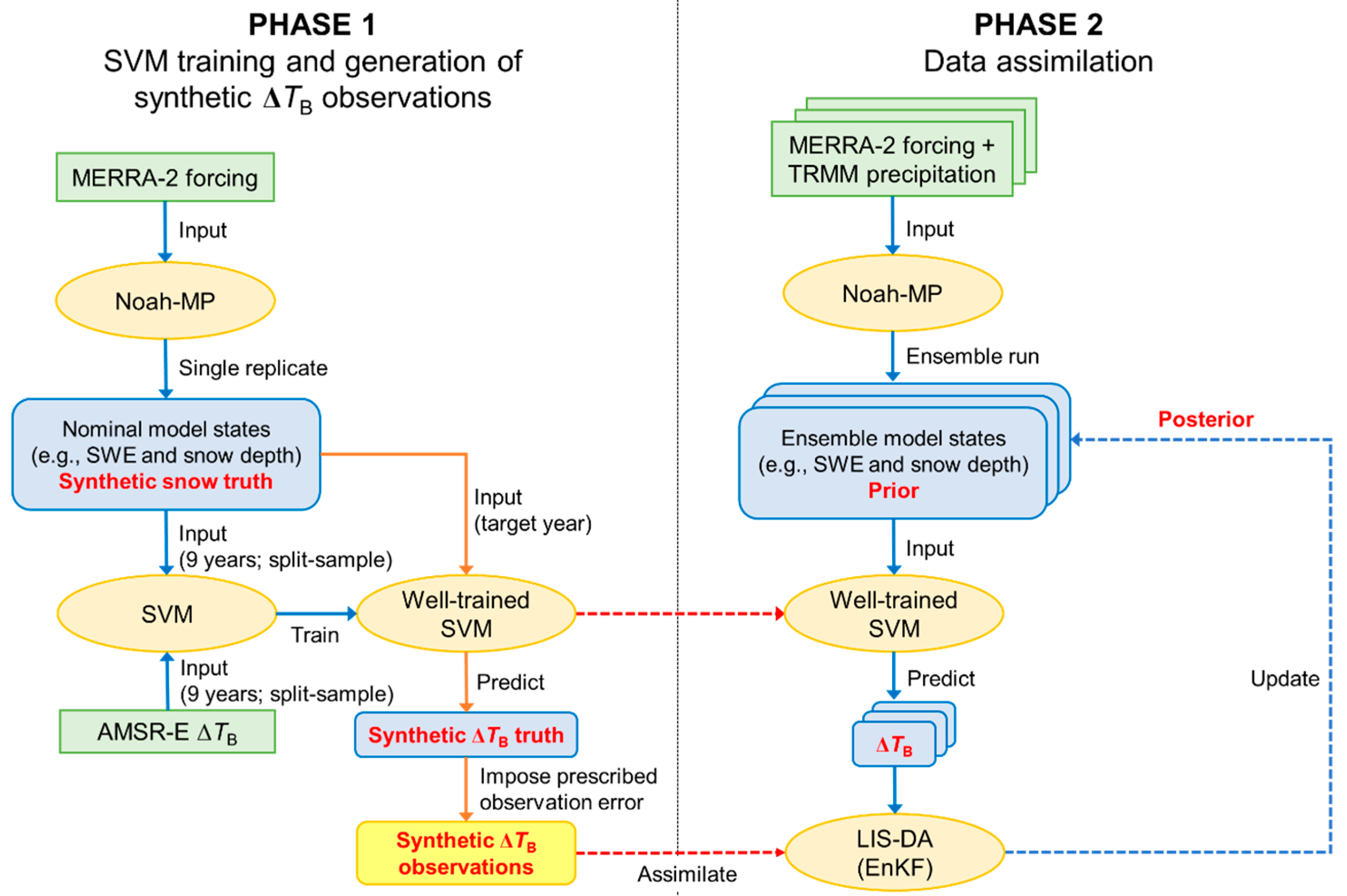
2.1. SVM-DA Framework and Synthetic Twin Experiment
2.2. Data Sets
2.3. Experimental Setup
2.3.1. Land Surface Model
2.3.2. SVM Training
2.3.3. Precipitation Bias Correction
2.3.4. Data Assimilation
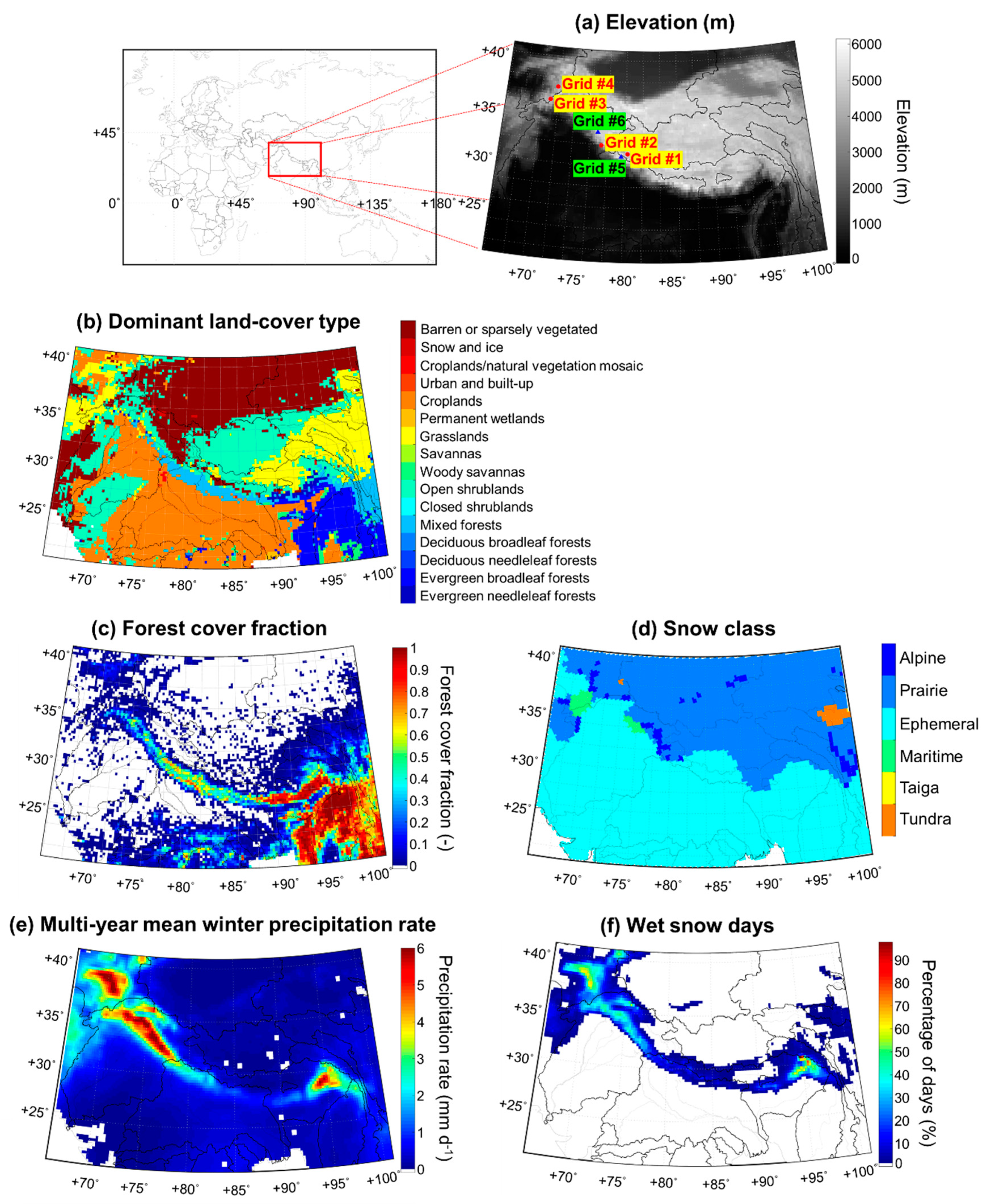
2.4. Study Area
3. Results and Discussion
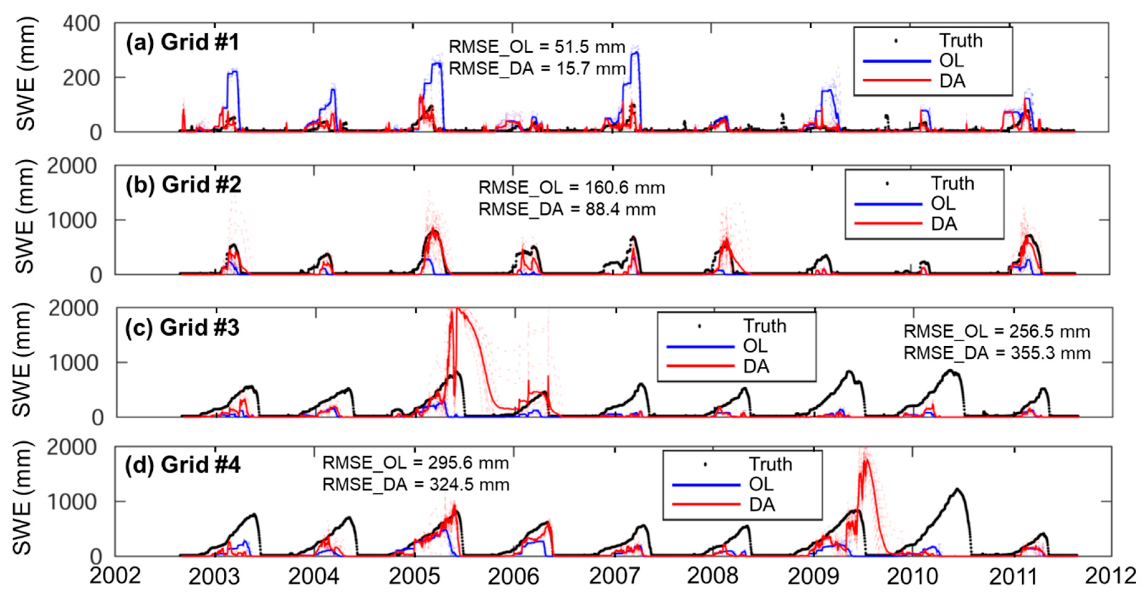
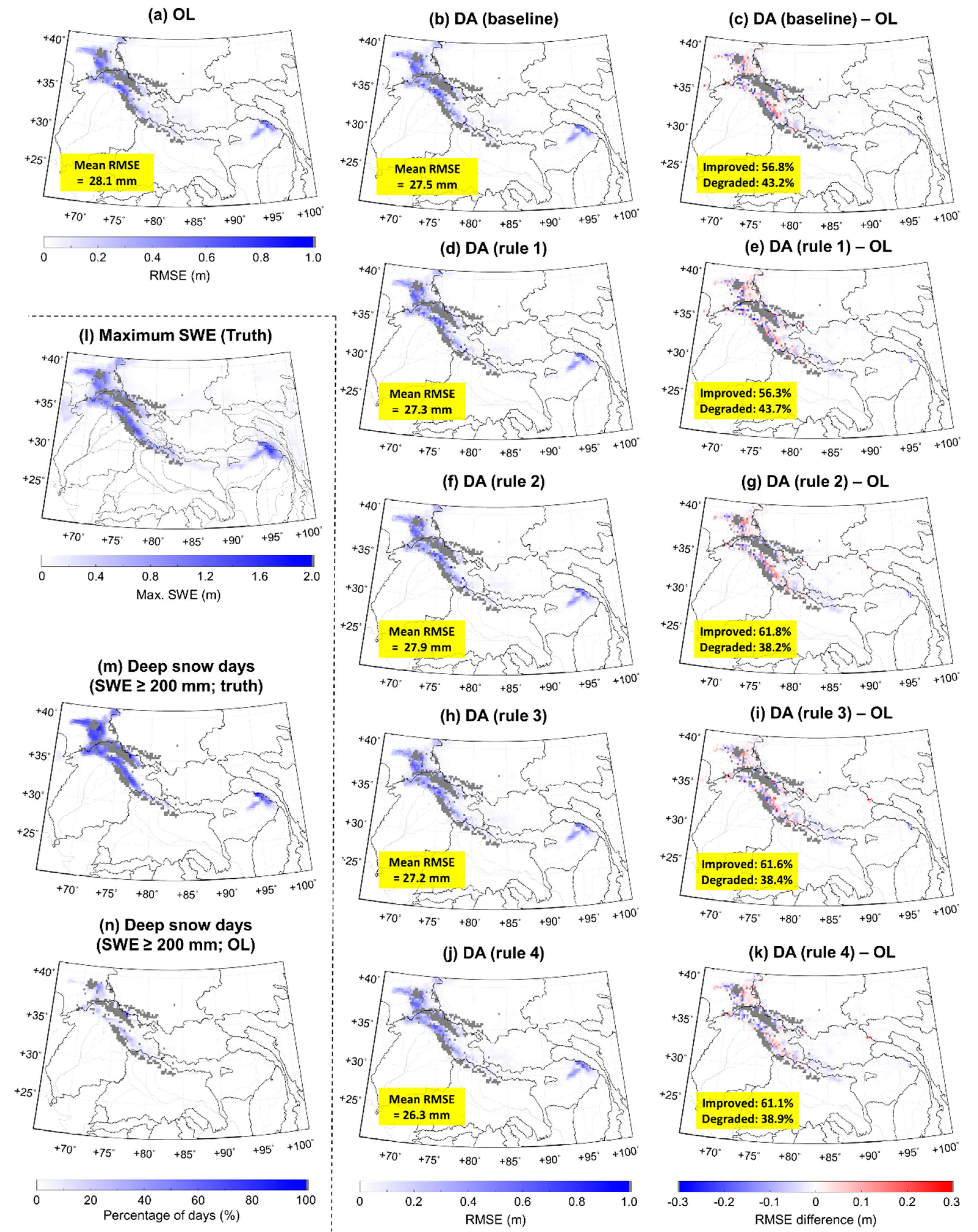
3.1. Performance of the SVM-DA Framework
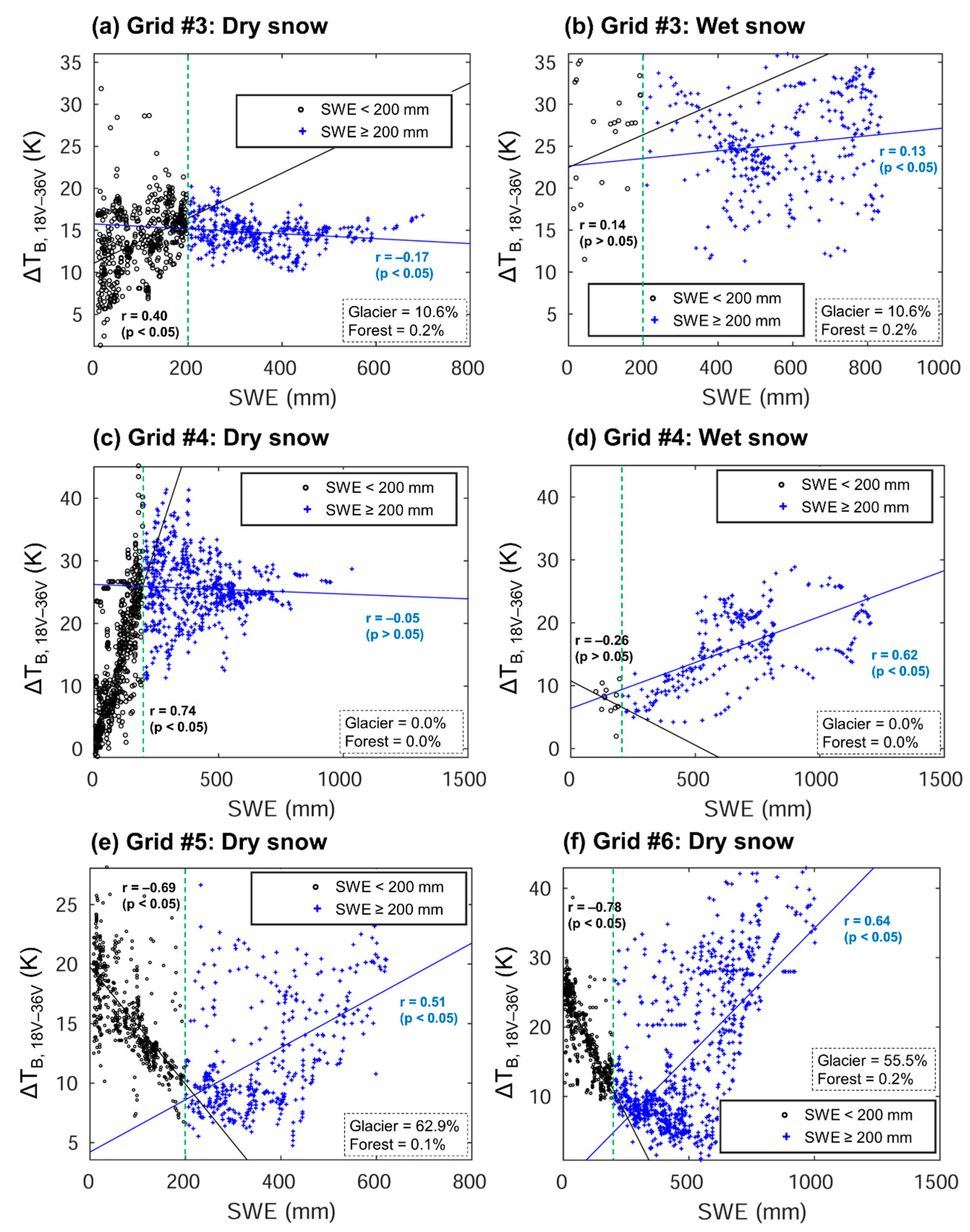
3.2. Limitations of ΔTB DA for Snow Estimation
3.3. Possible Improvements in DA Performance
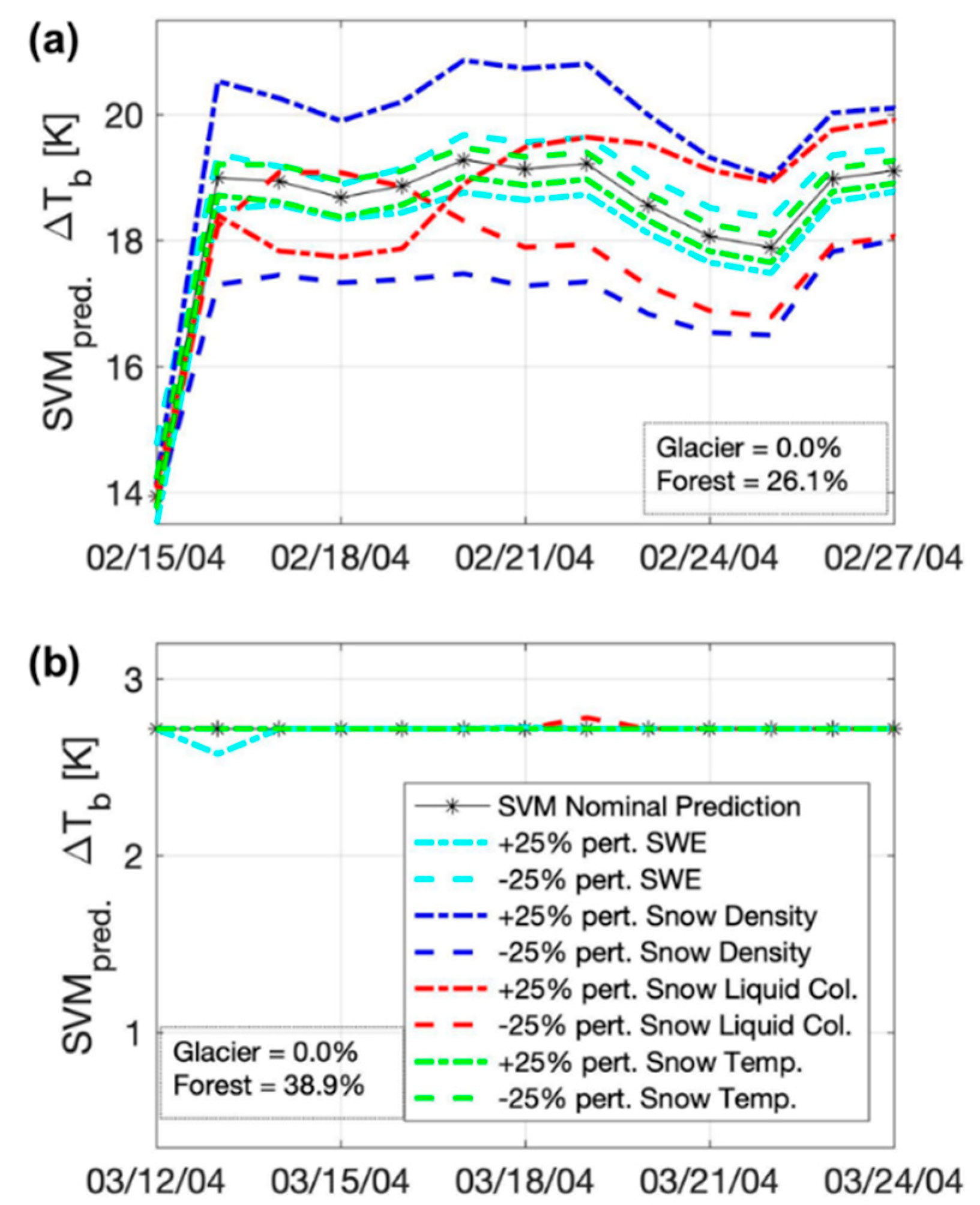
3.4. Controllability of Observation Operator
4. Summary and Conclusions
Supplementary Materials
Author Contributions
Funding
Acknowledgments
Conflicts of Interest
Abbreviations
| AMSR-E | Advanced Microwave Scanning Radiometer for Earth Observing System |
| ANN | Artificial neural network |
| AR(1) | First-order autoregressive model |
| CHIRPS-2 | Climate Hazards Group InfraRed Precipitation with Station data, version 2 |
| DA | Data assimilation |
| ECMWF | European Centre for Medium-Range Weather Forecasts |
| EnKF | Ensemble Kalman filter |
| GLIMS | Global Land Ice Measurements from Space |
| HMA | High Mountain Asia |
| IGBP | International Geosphere-Biosphere Program |
| IMS | Interactive Multisensor Snow and Ice Mapping System |
| LIS | Land Information System |
| LSM | Land surface model |
| MEaSUREs | Making Earth System Data Records for Use in Research Environments |
| MERRA-2 | Modern-Era Retrospective analysis for Research and Applications, version 2 |
| MODIS | Terra Moderate Resolution Imaging Spectroradiometer |
| NASA | National Aeronautics and Space Administration |
| NOAA/NESDIS | National Oceanic and Atmospheric Administration’s National Environmental Satellite Data and Information Service |
| Noah-MP | Noah Land Surface Model with multiparameterization options |
| NSC | Normalized sensitivity coefficient |
| OL | Open loop |
| PMW | Passive microwave |
| RTM | Radiative transfer model |
| SRTM | Shuttle Radar Topography Mission |
| SVM | Support vector machine |
| SWE | Snow water equivalent |
| TB | Brightness temperature |
| ΔTB | Brightness temperature spectral difference |
| TMPA | Multisatellite precipitation analysis |
| TRMM | Tropical Rainfall Measuring Mission |
References
- Immerzeel, W.W.; Van Beek, L.P.H.; Bierkens, M.F.P. Climate change will affect the Asian water towers. Science 2010, 328, 1382–1385. [Google Scholar] [CrossRef] [PubMed]
- Zhang, L.; Su, F.; Yang, D.; Hao, Z.; Tong, K. Discharge regime and simulation for the upstream of major rivers over Tibetan Plateau. J. Geophys. Res. Atmos. 2013, 118, 8500–8518. [Google Scholar] [CrossRef]
- Hewitt, K. The Karakoram anomaly? Glacier expansion and the “elevation effect” Karakoram Himalaya. Mt. Res. Dev. 2005, 25, 332–340. [Google Scholar] [CrossRef]
- Bolch, T.; Kulkarni, A.; Kaäb, A.; Huggel, C.; Paul, F.; Cogley, J.G.; Frey, H.; Kargel, J.S.; Fujita, K.; Scheel, M.; et al. The state and fate of Himalayan glaciers. Science 2012, 336, 310–314. [Google Scholar] [CrossRef] [PubMed]
- Farinotti, D.; Longuevergne, L.; Moholdt, G.; Duethmann, D.; Mölg, T.; Bolch, T.; Vorogushyn, S.; Güntner, A. Substantial glacier mass loss in the Tien Shan over the past 50 years. Nat. Geosci. 2015, 8, 716–722. [Google Scholar] [CrossRef]
- Buri, P.; Pellicciotti, F. Aspect controls the survival of ice cliffs on debris-covered glaciers. Proc. Natl. Acad. Sci. USA 2018, 115, 4369–4374. [Google Scholar] [CrossRef]
- Dehecq, A.; Gourmelen, N.; Gardner, A.S.; Brun, F.; Goldberg, D.; Nienow, P.W.; Berthier, E.; Vincent, C.; Wagnon, P.; Trouvé, E. Twenty-first century glacier slowdown driven by mass loss in High Mountain Asia. Nat. Geosci. 2019, 12, 22–27. [Google Scholar] [CrossRef]
- Durand, M.; Margulis, S.A. Feasibility test of multifrequency radiometric data assimilation to estimate snow water equivalent. J. Hydrometeor. 2006, 7, 443–457. [Google Scholar] [CrossRef]
- Durand, M.; Kim, E.J.; Margulis, S.A. Radiance assimilation shows promise for snowpack characterization. Geophys. Res. Lett. 2009, 36. [Google Scholar] [CrossRef]
- Chang, A.T.C.; Foster, J.L.; Hall, D.K. Nimbus-7 SMMR derived global snow cover parameters. Ann. Glaciol. 1987, 9, 39–44. [Google Scholar] [CrossRef]
- Toure, A.M.; Goïta, K.; Royer, A.; Kim, E.J.; Durand, M.; Margulis, S.A.; Lu, H. A case study of using a multilayered thermodynamical snow model for radiance assimilation. IEEE Trans. Geosci. Remote Sens. 2011, 49, 2828–2837. [Google Scholar] [CrossRef]
- Dechant, C.; Moradkhani, M. Radiance data assimilation for operational snow and streamflow forecasting. Adv. Water Resour. 2011, 34, 351–364. [Google Scholar] [CrossRef]
- Andreadis, K.M.; Lettenmaier, D.P. Implications of representing snowpack stratigraphy for the assimilation of passive microwave satellite observations. J. Hydrometeor. 2012, 13, 1493–1506. [Google Scholar] [CrossRef]
- Langlois, A.; Royer, A.; Derksen, C.; Montpetit, B.; Dupont, F.; Goïta, K. Coupling the snow thermodynamic model SNOWPACK with the microwave emission model of layered snowpacks for subarctic and arctic snow water equivalent retrievals. Water Resour. Res. 2012, 48. [Google Scholar] [CrossRef]
- Che, T.; Li, X.; Jin, R.; Huang, C. Assimilating passive microwave remote sensing data into a land surface model to improve the estimation of snow depth. Remote Sens. Environ. 2014, 143, 54–63. [Google Scholar] [CrossRef]
- Kwon, Y.; Yang, Z.-L.; Zhao, L.; Hoar, T.J.; Toure, A.M.; Rodell, M. Estimating snow water storage in North America using CLM4, DART, and snow radiance data assimilation. J. Hydrometeor. 2016, 17, 2853–2874. [Google Scholar] [CrossRef]
- Kwon, Y.; Yang, Z.-L.; Hoar, T.J.; Toure, A.M. Improving the radiance assimilation performance in estimating snow water storage across snow and land-cover types in North America. J. Hydrometeor. 2017, 18, 651–668. [Google Scholar] [CrossRef]
- Larue, F.; Royer, A.; De Sève, D.; Roy, A.; Cosme, E. Assimilation of passive microwave AMSR-2 satellite observations in a snowpack evolution model over northeastern Canada. Hydrol. Earth Syst. Sci. 2018, 22, 5711–5734. [Google Scholar] [CrossRef]
- Kim, R.S.; Durand, M.; Li, D.; Baldo, E.; Margulis, S.A.; Dumont, M.; Morin, S. Estimating alpine snow depth by combining multifrequency passive radiance observations with ensemble snowpack modeling. Remote Sens. Environ. 2019, 226, 1–15. [Google Scholar] [CrossRef]
- Forman, B.A.; Reichle, R.H.; Derksen, C. Estimating passive microwave brightness temperature over snow-covered land in North America using a land surface model and an artificial neural network. IEEE Trans. Geosci. Remote Sens. 2014, 52, 235–248. [Google Scholar] [CrossRef]
- Forman, B.A.; Reichle, R.H. Using a support vector machine and a land surface model to estimate large-scale passive microwave brightness temperatures over snow-covered land in North America. IEEE J. Selec. Top. Appl. Earth Obs. Remote Sens. 2015, 8, 4431–4441. [Google Scholar] [CrossRef]
- Xue, Y.; Forman, B.A. Comparison of passive microwave brightness temperature prediction sensitivities over snow-covered land in North America using machine learning algorithms and the Advanced Microwave Scanning Radiometer. Remote Sens. Environ. 2015, 170, 153–165. [Google Scholar] [CrossRef]
- Xue, Y.; Forman, B.A.; Reichle, R.H. Estimating snow mass in North America through assimilation of Advanced Microwave Scanning Radiometer brightness temperature observations using the Catchment land surface model and support vector machines. Water Resour. Res. 2018, 54, 6488–6509. [Google Scholar] [CrossRef]
- Durand, M.; Kim, E.J.; Margulis, S.A. Quantifying uncertainty in modeling snow microwave radiance for a mountain snowpack at the point-scale, including stratigraphic effects. IEEE Trans. Geosci. Remote Sens. 2008, 46, 1753–1767. [Google Scholar] [CrossRef]
- Kumar, S.V.; Peters-Lidard, C.D.; Tian, Y.; Houser, P.R.; Geiger, J.; Olden, S.; Lighty, L.; Eastman, J.L.; Doty, B.; Dirmeyer, P.; et al. Land information system: An interoperable framework for high resolution land surface modeling. Environ. Modell. Softw. 2006, 21, 1402–1415. [Google Scholar] [CrossRef]
- Peters-Lidard, C.D.; Houser, P.R.; Tian, Y.; Kumar, S.V.; Geiger, J.; Olden, S.; Lighty, L.; Doty, B.; Dirmeyer, P.; Adams, J.; et al. High-performance Earth system modeling with NASA/GSFC’s Land Information System. Innov. Syst. Softw. Eng. 2007, 3, 157–165. [Google Scholar] [CrossRef]
- Kumar, S.; Peters-Lidard, C.; Tian, Y.; Reichle, R.H.; Geiger, J.; Alonge, C.; Eylander, J.; Houser, P. An integrated hydrologic modeling and data assimilation framework. Computer 2008, 41, 52–59. [Google Scholar] [CrossRef]
- Niu, G.-Y.; Yang, Z.-L.; Mitchell, K.E.; Chen, F.; Ek, M.B.; Barlage, M.; Kumar, A.; Manning, K.; Niyogi, D.; Rosero, E.; et al. The community Noah land surface model with multiparameterization options (Noah-MP): 1. Model description and evaluation with local-scale measurements. J. Geophys. Res. 2011, 116. [Google Scholar] [CrossRef]
- Yang, Z.-L.; Niu, G.-Y.; Mitchell, K.E.; Chen, F.; Ek, M.B.; Barlage, M.; Longuevergne, L.; Manning, K.; Niyogi, D.; Tewari, M.; et al. The community Noah land surface model with multiparameterization options (Noah-MP): 2. Evaluation over global river basins. J. Geophys. Res. 2011, 116. [Google Scholar] [CrossRef]
- Reichle, R.H.; Koster, R.D. Assessing the impact of horizontal error correlations in background fields on soil moisture estimation. J. Hydrometeor. 2003, 4, 1229–1242. [Google Scholar] [CrossRef]
- Clark, M.P.; Slater, A.G.; Barrett, A.P.; Hay, L.E.; McCabe, G.J.; Rajagopalan, B.; Leavesley, G.H. Assimilation of snow covered area information into hydrologic and land-surface models. Adv. Water Resour. 2006, 29, 1209–1221. [Google Scholar] [CrossRef]
- Forman, B.A.; Reichle, R.H. The spatial scale of model errors and assimilated retrievals in a terrestrial water storage assimilation system. Water Resour. Res. 2013, 49. [Google Scholar] [CrossRef]
- Kumar, S.V.; Reichle, R.H.; Peters-Lidard, C.D.; Koster, R.D.; Zhan, X.; Crow, W.T.; Eylander, J.B.; Houser, P.R. A land surface data assimilation framework using the land information system: Description and applications. Adv. Water Resour. 2008, 31, 1419–1432. [Google Scholar] [CrossRef]
- Vapnik, V.N. An overview of statistical learning theory. IEEE Trans. Neural Netw. 1999, 10, 988–999. [Google Scholar] [CrossRef] [PubMed]
- Cherkassky, V.; Ma, Y. Practical selection of SVM parameters and noise estimation for SVM regression. Neural Netw. 2004, 17, 113–126. [Google Scholar] [CrossRef]
- Chang, C.C.; Lin, C.J. LIBSVM: A library for support vector machines. ACM Trans. Intell. Syst. Technol. 2011, 2, 1–27. [Google Scholar] [CrossRef]
- Bosilovich, M.G.; Lucchesi, R.; Suarez, M. MERRA-2: Initial Evaluation of the Climate; Technical Report No. 104606; NASA: Washington, DC, USA, 2015; p. 73.
- Huffman, G.J.; Bolvin, D.T.; Nelkin, E.J.; Wolff, D.B.; Adler, R.F.; Gu, G.; Hong, Y.; Bowman, K.P.; Stocker, E.F. The TRMM multisatellite precipitation analysis (TMPA): Quasi-global, multiyear, combined-sensor precipitation estimates at fine scales. J. Hydrometeor. 2007, 8, 38–55. [Google Scholar] [CrossRef]
- Evensen, G. Sequential data assimilation with a nonlinear quasi-geostrophic model using Monte Carlo methods to forecast error statistics. J. Geophys. Res. 1994, 99, 10143–10162. [Google Scholar] [CrossRef]
- Reichle, R.H.; Walker, J.P.; Koster, R.D.; Houser, P.R. Extended versus ensemble Kalman filtering for land data assimilation. J. Hydrometeor. 2002, 3, 728–740. [Google Scholar] [CrossRef]
- Brodzik, M.J.; Long, D.G.; Hardman, M.A.; Paget, A.; Armstrong, R. MEaSUREs Calibrated Enhanced-Resolution Passive Microwave Daily EASE-Grid 2.0 Brightness Temperature ESDR, Version 1; NASA National Snow and Ice Data Center Distributed Active Archive Center: Boulder, CO, USA, 2016. [Google Scholar]
- Yoon, Y.; Kumar, S.V.; Forman, B.A.; Zaitchik, B.F.; Kwon, Y.; Qian, Y.; Rupper, S.; Maggioni, V.; Houser, P.; Kirschbaum, D.; et al. Evaluating the uncertainty of terrestrial water budget components over High Mountain Asia. Front. Earth Sci. 2019, 7, 120. [Google Scholar] [CrossRef]
- Funk, C.; Peterson, P.; Landsfeld, M.; Pedreros, D.; Verdin, J.; Shukla, S.; Husak, G.; Rowland, J.; Harrison, L.; Hoell, A.; et al. The climate hazards infrared precipitation with stations–A new environmental record for monitoring extremes. Sci. Data 2015, 2, 150066. [Google Scholar] [CrossRef] [PubMed]
- Molteni, F.; Buizza, R.; Palmer, T.N.; Petroliagis, T. The ECMWF ensemble prediction system: Methodology and validation. Q. J. R. Meteorol. Soc. 1996, 122, 73–119. [Google Scholar] [CrossRef]
- Ahmad, J.A.; Forman, B.A.; Kwon, Y. Analyzing machine learning predictions of passive microwave brightness temperature spectral difference over snow-covered terrain in High Mountain Asia. Front. Earth Sci. 2019, 7, 212. [Google Scholar] [CrossRef]
- Farr, T.G.; Rosen, P.A.; Caro, E.; Crippen, R.; Duren, R.; Hensley, S.; Kobrick, M.; Paller, M.; Rodriguez, E.; Roth, L.; et al. The shuttle radar topography mission. Rev. Geophys. 2007, 45. [Google Scholar] [CrossRef]
- Friedl, M.A.; McIver, D.K.; Hodges, J.C.F.; Zhang, X.Y.; Muchoney, D.; Strahler, A.H.; Woodcock, C.E.; Gopal, S.; Schneider, A.; Cooper, A.; et al. Global land cover mapping from MODIS: Algorithms and early results. Remote Sens. Environ. 2002, 83, 287–302. [Google Scholar] [CrossRef]
- Hengl, T.; de Jesus, J.M.; MacMillan, R.A.; Batjes, N.H.; Heuvelink, G.B.M.; Ribeiro, E.; Samuel-Rosa, A.; Kempen, B.; Leenaars, J.G.B.; Walsh, M.G.; et al. SoilGrids1km–Global soil information based on automated mapping. PLoS ONE 2014, 9, e105992. [Google Scholar] [CrossRef]
- Ball, J.T.; Woodrow, I.E.; Berry, J.A. A model predicting stomatal conductance and its contribution to the control of photosynthesis under different environmental conditions. In Process in Photosynthesis Research; Biggins, J., Ed.; Martinus Nijhoff: Dordrecht, The Netherlands, 1987; pp. 221–234. ISBN 978-94-017-0521-9. [Google Scholar]
- Chen, F.; Dudhia, J. Coupling an advanced land surface-hydrology model with the Penn State-NCAR MM5 modeling system. Part I: Model implementation and sensitivity. Mon. Weather Rev. 2001, 129, 569–585. [Google Scholar] [CrossRef]
- Niu, G.-Y.; Yang, Z.-L.; Dickinson, R.E.; Gulden, L.E.; Su, H. Development of a simple groundwater model for use in climate models and evaluation with Gravity Recovery and Climate Experiment data. J. Geophys. Res. 2007, 112. [Google Scholar] [CrossRef]
- Brutsaert, W.A. Evaporation into the Atmosphere; D. Reidel: Dordrecht, The Netherlands, 1982. [Google Scholar]
- Niu, G.-Y.; Yang, Z.-L. Effects of frozen soil on snowmelt runoff and soil water storage at a continental scale. J. Hydrometeorol. 2006, 7, 937–952. [Google Scholar] [CrossRef]
- Yang, R.; Friedl, M.A. Modeling the effects of three-dimensional vegetation structure on surface radiation and energy balance in boreal forests. J. Geophys. Res. 2003, 108, 8615. [Google Scholar] [CrossRef]
- Niu, G.-Y.; Yang, Z.-L. The effects of canopy processes on snow surface energy and mass balances. J. Geophys. Res. 2004, 109. [Google Scholar] [CrossRef]
- Yang, Z.-L.; Dickinson, R.E. Description of the Biosphere-Atmosphere Transfer Scheme (BATS) for the soil moisture workshop and evaluation of its performance. Global Planet. Chang. 1996, 13, 117–134. [Google Scholar] [CrossRef]
- Jordan, R. A One-Dimensional Temperature Model for a Snow Cover. Technical Documentation for SNTHERM.89; Technical Report No. 91-16; U.S. Army Corps of Engineers: Washington, DC, USA, 1991.
- Derksen, C. The contribution of AMSR-E 18.7 and 10.7 GHz measurements to improved boreal forest snow water equivalent retrievals. Remote Sens. Environ. 2008, 112, 2701–2710. [Google Scholar] [CrossRef]
- Kelly, R. The AMSR-E snow depth algorithm: Description and initial results. J. Remote Sens. Soc. Jpn. 2009, 29, 307–317. [Google Scholar] [CrossRef]
- Derksen, C.; Toose, P.; Rees, A.; Wang, L.; English, M.; Walker, A.; Sturm, M. Development of a tundra-specific snow water equivalent retrieval algorithm for satellite passive microwave data. Remote Sens. Environ. 2010, 114, 1699–1709. [Google Scholar] [CrossRef]
- Foster, J.L.; Hall, D.K.; Eylander, J.B.; Riggs, G.A.; Nghiem, S.V.; Tedesco, M.; Kim, E.; Montesano, P.M.; Kelly, R.E.J.; Casey, K.A.; et al. A blended global snow product using visible, passive microwave, and scatterometer satellite data. Int. J. Remote Sens. 2011, 32, 1371–1395. [Google Scholar] [CrossRef]
- Pulliainen, J.; Kärnä, J.-P.; Hallikainen, M. Development of geophysical retrieval algorithms for the MIMR. IEEE Trans. Geosci. Remote Sens. 1993, 31, 268–277. [Google Scholar] [CrossRef]
- Turner, D.D.; Clough, S.A.; Liljegren, J.C.; Clothiaux, E.E.; Cady-Pereira, K.E.; Gaustad, K.L. Retrieving liquid water path and precipitable water vapor from the Atmospheric Radiation Measurement (ARM) microwave radiometers. IEEE Trans. Geosci. Remote Sens. 2007, 45, 3680–3690. [Google Scholar] [CrossRef]
- Walker, A.; Goodison, B. Discrimination of a wet snow cover using passive microwave satellite data. Ann. Glaciol. 1993, 17, 307–311. [Google Scholar] [CrossRef]
- Xue, Y.; Forman, B.A. Atmospheric and forest decoupling of passive microwave brightness temperature observations over snow-covered terrain in North America. IEEE J. Selec. Top. Appl. Earth Obs. Remote Sens. 2017, 10, 3172–3189. [Google Scholar] [CrossRef]
- Abdalati, W.; Steffen, K. Passive microwave-derived snow melt regions on the Greenland ice sheet. Geophys. Res. Lett. 1995, 22, 787–790. [Google Scholar] [CrossRef]
- Savoie, M.H.; Armstrong, R.L.; Brodzik, M.J.; Wang, J.R. Atmospheric corrections for improved satellite passive microwave snow cover retrievals over the Tibet Plateau. Remote Sens. Environ. 2009, 113, 2661–2669. [Google Scholar] [CrossRef]
- Clifford, D. Global estimates of snow water equivalent from passive microwave instruments: History, challenges and future developments. Int. J. Remote Sens. 2010, 31, 3707–3726. [Google Scholar] [CrossRef]
- Sturm, M.; Holmgren, J.; Liston, G.E. A seasonal snow cover classification system for local to regional applications. J. Clim. 1995, 8, 1261–1283. [Google Scholar] [CrossRef]
- Ramsay, B. The interactive multisensory snow and ice mapping system. Hydrol. Proc. 1998, 12, 1537–1546. [Google Scholar] [CrossRef]
- Helfrich, S.R.; McNamara, D.; Ramsay, B.H.; Baldwin, T.; Kasheta, T. Enhancements to, and forthcoming developments in the Interactive Multisensor Snow and Ice Mapping System (IMS). Hydrol. Proc. 2007, 21, 1576–1586. [Google Scholar] [CrossRef]
- Reichle, R.H.; Koster, R.D.; Liu, P.; Mahanama, P.P.; Njoku, E.G.; Owe, M. Comparison and assimilation of global soil moisture retrievals from the Advanced Microwave Scanning Radiometer for the Earth Observing System (AMSR-E) and the Scanning Multichannel Microwave Radiometer (SMMR). J. Geophys. Res. 2007, 112. [Google Scholar] [CrossRef]
- Reichle, R.H.; Crow, W.T.; Keppenne, C.L. An adaptive ensemble Kalman filter for soil moisture data assimilation. Water Resour. Res. 2008, 44. [Google Scholar] [CrossRef]
- Kumar, S.V.; Reichle, R.H.; Koster, R.D.; Crow, W.T.; Peters-Lidard, C.D. Role of subsurface physics in the assimilation of surface soil moisture observations. J. Hydrometeor. 2009, 10, 1534–1547. [Google Scholar] [CrossRef]
- Kumar, S.V.; Zaitchik, B.F.; Peters-Lidard, C.D.; Rodell, M.; Reichle, R.; Li, B.; Jasinski, M.; Mocko, D.; Getirana, A.; De Lannoy, G.; et al. Assimilation of gridded GRACE terrestrial water storage estimates in the North American Land Data Assimilation System. J. Hydrometeor. 2016, 17, 1951–1972. [Google Scholar] [CrossRef]
- Forman, B.A.; Reichle, R.H.; Rodell, M. Assimilation of terrestrial water storage from GRACE in a snow-dominated basin. Water Resour. Res. 2012, 48. [Google Scholar] [CrossRef]
- Durand, M.; Margulis, S.A. Correcting first-order errors in snow water equivalent estimates using a multifrequency, multiscale radiometric data assimilation scheme. J. Geophys. Res. 2007, 112. [Google Scholar] [CrossRef]
- Wester, P.; Mishra, A.; Mukherji, A.; Shrestha, A.B. The Hindu Kush Himalaya Assessment—Mountains, Climate Change, Sustainability and People; Springer Nature Switzerland AG: Cham, Switzerland, 2018. [Google Scholar]
- GLIMS; National Snow and Ice Data Center. Global Land Ice Measurements from Space Glacier Database; National Snow and Ice Data Center: Boulder, CO, USA, 2005.
- Kim, E.J.; England, A.W. A yearlong comparison of plot-scale and satellite footprint-scale 19 and 37 GHz brightness temperature of the Alaskan North Slope. J. Geophys. Res. 2003, 108, 4388–4403. [Google Scholar] [CrossRef]
- Schanda, E.; Mätzler, C.; Kunzi, K. Microwave remote sensing of snow cover. Int. J. Remote Sens. 1983, 4, 149–158. [Google Scholar] [CrossRef]
- Lemmetyinen, J.; Derksen, C.; Toose, P.; Proksch, M.; Pulliainen, J.; Kontu, A.; Rautiainen, K.; Seppänen, J.; Hallikainen, M. Simulating seasonally and spatially varying snow cover brightness temperature using HUT snow emission model and retrieval of a microwave effective grain size. Remote Sens. Environ. 2015, 156, 71–95. [Google Scholar] [CrossRef]
- Fuller, M.C.; Derksen, C.; Yackel, J. Plot scale passive microwave measurements and modeling of layered snow using the multi-layered HUT model. Can. J. Remote Sens. 2015, 41, 219–231. [Google Scholar] [CrossRef]
- Cumming, W.A. The dielectric properties of ice and snow at 3.2 centimeters. J. Appl. Phys. 1952, 23, 768–773. [Google Scholar] [CrossRef]
- Grenfell, T.C. Surface-based passive microwave studies of multiyear sea ice. J. Geophys. Res. 1992, 97, 3485–3501. [Google Scholar] [CrossRef]
- Eppler, D.T.; Farmer, D.; Lohanick, A.W.; Anderson, M.R.; Cavalieri, D.J.; Comiso, J.; Gloersen, P.; Garrity, C.; Grenfell, T.C.; Hallikainen, M.; et al. Passive microwave signatures of sea ice. In Microwave Remote Sensing of Sea Ice; Carsey, F.D., Ed.; American Geophysical Union: Washington, DC, USA, 1992; pp. 47–71. [Google Scholar]
- Foster, J.L.; Chang, A.T.C.; Hall, D.K.; Rango, A. Derivation of snow water equivalent in boreal forests using microwave radiometry. Arctic 1991, 44, 147–152. [Google Scholar] [CrossRef]
- Chang, A.T.C.; Foster, J.L.; Hall, D.K. Effects of forest on the snow parameters derived from microwave measurements during the BOREAS winter field experiment. Hydrol. Proc. 1996, 10, 1565–1574. [Google Scholar] [CrossRef]
- Pampaloni, P. Microwave radiometry of forests. Waves Random Media 2004, 14, S275–S298. [Google Scholar] [CrossRef]
- Hallikainen, M.T.; Jolma, P.A. Comparison of algorithms for retrieval of snow water equivalent from Nimbus-7 SMMR data in Finland. IEEE Trans. Geosci. Remote Sens. 1992, 30, 124–131. [Google Scholar] [CrossRef]
- Roy, A.; Royer, A.; Wigneron, J.-P.; Langlois, A.; Bergeron, J.; Cliche, P. A simple parameterization for a boreal forest radiative transfer model at microwave frequencies. Remote Sens. Environ. 2012, 124, 371–383. [Google Scholar] [CrossRef]
- Pellarin, T.; Kerr, Y.H.; Wigneron, J.-P. Global simulations of brightness temperature at 6.6 and 10.7 GHz over land based on SMMR data set analysis. IEEE Trans. Geosci. Remote Sens. 2006, 44, 2492–2505. [Google Scholar] [CrossRef]
- Grant, J.P.; Saleh, K.; Wigneron, J.-P.; Guglielmetti, M.; Kerr, Y.H.; Schwank, M.; Skou, N.; Van deGriend, A. Calibration of the L-MEB model over a coniferous and a deciduous forest. IEEE Trans. Geosci. Remote Sens. 2008, 46, 808–818. [Google Scholar] [CrossRef]
- Kwon, Y.; Toure, A.M.; Yang, Z.-L.; Rodell, M.; Picard, G. Error characterization of coupled land surface–Radiative transfer models for snow microwave radiance assimilation. IEEE Trans. Geosci. Remote Sens. 2015, 53, 5247–5268. [Google Scholar] [CrossRef]
- Sandells, M.; Essery, R.; Rutter, N.; Wake, L.; Leppänen, L.; Lemmetyinen, J. Microstructure representation of snow in coupled snowpack and microwave emission models. The Cryosphere 2017, 11, 229–246. [Google Scholar] [CrossRef]
- Picard, G.; Sandells, M.; Löwe, H. SMRT: An active-passive microwave radiative transfer model for snow with multiple microstructure and scattering formulations (v1.0). Geosci. Model Dev. 2018, 11, 2763–2788. [Google Scholar] [CrossRef]
- Roy, A.; Picard, G.; Royer, A.; Montpetit, B.; Dupont, F.; Langlois, A.; Derksen, C.; Champollion, N. Brightness temperature simulations of the Canadian seasonal snowpack driven by measurements of the snow specific surface area. IEEE Trans. Geosci. Remote Sens. 2013, 51, 4692–4704. [Google Scholar] [CrossRef]
- Ogata, K. Modern Control Engineering; Prentice Hall International Inc.: Upper Saddle River, NJ, USA, 1997. [Google Scholar]
- Gelb, A. Applied Optimal Estimation; M.I.T. Press: Cambridge, MA, USA, 1974. [Google Scholar]
- Pulvirenti, L.; Pierdicca, N.; Marzano, F.S. Topographic effects on the surface emissivity of a mountainous area observed by a spaceborne microwave radiometer. Sensors 2008, 8, 1459–1474. [Google Scholar] [CrossRef]
- Rodríguez-Fernández, N.; de Rosnay, P.; Albergel, C.; Richaume, P.; Aires, F.; Prigent, C.; Kerr, Y. SMOS Neural Network Soil Moisture Data Assimilation in a Land Surface Model and Atmospheric Impact. Remote Sens. 2019, 11, 1334. [Google Scholar] [CrossRef]


| Process | Selected Option | References |
|---|---|---|
| Vegetation | Dynamic | - |
| Canopy stomatal resistance | Ball–Berry | [49] |
| Soil moisture factor for stomatal resistance | Noah type using soil moisture | [50] |
| Runoff and groundwater | SIMGM a | [51] |
| Surface layer drag coefficient | M-O b | [52] |
| Supercooled liquid water (or ice fraction) in frozen soil | NY06 | [53] |
| Frozen soil permeability | NY06 | [53] |
| Radiation transfer | Modified two-stream | [54,55] |
| Ground snow surface albedo | BATS c | [56] |
| Partitioning precipitation into rainfall and snowfall | Jordan91 | [57] |
| Lower boundary condition of soil temperature | Original Noah scheme | - |
| Snow and soil temperature time scheme (only the first layer) | Semi-implicit | - |
| Perturbed Meteorological Forcing | Type | Std Dev | AR(1) | Cross-Correlations with Perturbations in | |||
|---|---|---|---|---|---|---|---|
| P | SW | LW | Tair | ||||
| Precipitation (P) | M | 0.5 | 1 day | − | −0.8 | 0.5 | −0.1 |
| Shortwave radiation (SW) | M | 0.3 | 1 day | −0.8 | – | −0.5 | 0.3 |
| Longwave radiation (LW) | A | 50 W m−2 | 1 day | 0.5 | −0.5 | – | 0.6 |
| Near surface air temperature (Tair) | A | 1 K | 1 day | −0.1 | 0.3 | 0.6 | – |
| Grid ID | Latitude | Longitude | Elevation a (m) | Dominant Land-Cover Type b | Forest Fraction b (%) | Glacier Fraction c (%) |
|---|---|---|---|---|---|---|
| 1 | 31.125°N | 80.375°E | 4659 | Open shrublands | 0 | 0 |
| 2 | 31.875°N | 77.375°E | 2986 | Mixed forests | 54.4 | 0.96 |
| 3 | 35.875°N | 71.125°E | 4528 | Barren or sparsely vegetated | 0.2 | 10.6 |
| 4 | 37.125°N | 71.875°E | 4053 | Open shrublands | 0 | 0 |
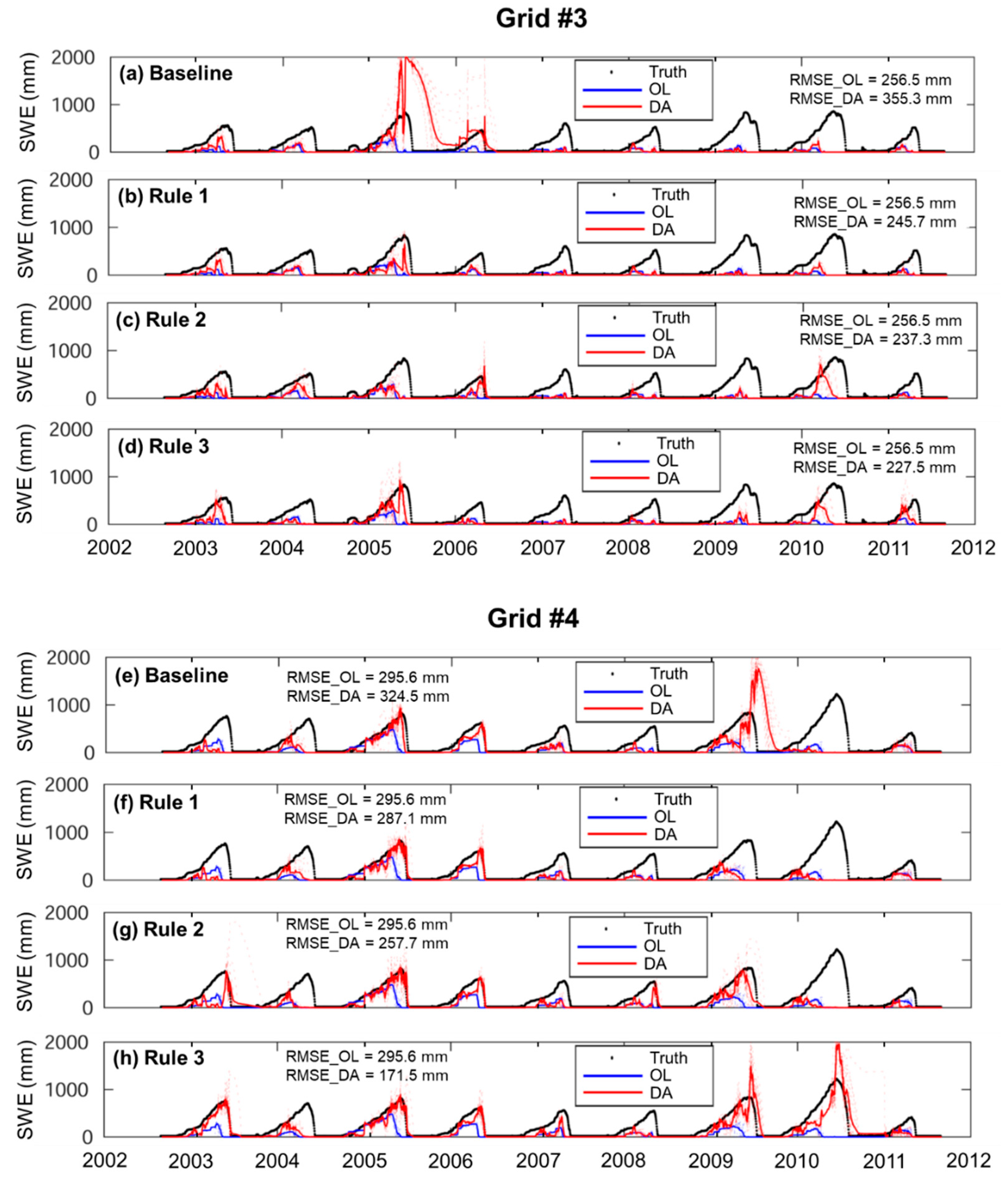
| Applied Rule | Description |
|---|---|
| Rule 1 | Update SWE only when the standard deviation of the predicted ΔTB is larger than 0.05 K |
| Rule 2 | Add a thin layer (i.e., 5 mm SWE) when the observed ΔTB is greater than 5 K but the simulated SWE is 0 mm. |
| Rule 3 | Rule 1 + Rule 2 |
| Rule 4 | Rule 3 + Suppress the analysis update when SWE of one or more of the ensemble members is greater than 500 mm. |
© 2019 by the authors. Licensee MDPI, Basel, Switzerland. This article is an open access article distributed under the terms and conditions of the Creative Commons Attribution (CC BY) license (http://creativecommons.org/licenses/by/4.0/).
Share and Cite
Kwon, Y.; Forman, B.A.; Ahmad, J.A.; Kumar, S.V.; Yoon, Y. Exploring the Utility of Machine Learning-Based Passive Microwave Brightness Temperature Data Assimilation over Terrestrial Snow in High Mountain Asia. Remote Sens. 2019, 11, 2265. https://doi.org/10.3390/rs11192265
Kwon Y, Forman BA, Ahmad JA, Kumar SV, Yoon Y. Exploring the Utility of Machine Learning-Based Passive Microwave Brightness Temperature Data Assimilation over Terrestrial Snow in High Mountain Asia. Remote Sensing. 2019; 11(19):2265. https://doi.org/10.3390/rs11192265
Chicago/Turabian StyleKwon, Yonghwan, Barton A. Forman, Jawairia A. Ahmad, Sujay V. Kumar, and Yeosang Yoon. 2019. "Exploring the Utility of Machine Learning-Based Passive Microwave Brightness Temperature Data Assimilation over Terrestrial Snow in High Mountain Asia" Remote Sensing 11, no. 19: 2265. https://doi.org/10.3390/rs11192265
APA StyleKwon, Y., Forman, B. A., Ahmad, J. A., Kumar, S. V., & Yoon, Y. (2019). Exploring the Utility of Machine Learning-Based Passive Microwave Brightness Temperature Data Assimilation over Terrestrial Snow in High Mountain Asia. Remote Sensing, 11(19), 2265. https://doi.org/10.3390/rs11192265