Utilizing Satellite Surface Soil Moisture Data in Calibrating a Distributed Hydrological Model Applied in Humid Regions Through a Multi-Objective Bayesian Hierarchical Framework

Abstract

The traditional calibration objective of hydrological models is to optimize streamflow simulations. To identify the value of satellite soil moisture data in calibrating hydrological models, a new objective of optimizing soil moisture simulations has been added to bring in satellite data. However, it leads to problems: (i) how to consider the trade-off between various objectives; (ii) how to consider the uncertainty these satellite data bring in. Among existing methods, the multi-objective Bayesian calibration framework has the potential to solve both problems but is more suitable for lumped models since it can only deal with constant variances (in time and space) of model residuals. In this study, to investigate the utilization of a soil moisture product from the Soil Moisture Active Passive (SMAP) satellite in calibrating a distributed hydrological model, the DEM (Digital Elevation Model) -based Distributed Rainfall-Runoff Model (DDRM), a multi-objective Bayesian hierarchical framework is employed in two humid catchments of southwestern China. This hierarchical framework is superior to the non-hierarchical framework when applied to distributed models since it considers the spatial and temporal residual heteroscedasticity of distributed model simulations. Taking the streamflow-based single objective calibration as the benchmark, results of adding satellite soil moisture data in calibration show that (i) there is less uncertainty in streamflow simulations and better performance of soil moisture simulations either in time and space; (ii) streamflow simulations are largely affected, while soil moisture simulations are slightly affected by weights of objectives. Overall, the introduction of satellite soil moisture data in addition to observed streamflow in calibration and putting more weights on the streamflow calibration objective lead to better hydrological performance. The multi-objective Bayesian hierarchical framework implemented here successfully provides insights into the value of satellite soil moisture data in distributed model calibration.

1. Introduction

It is well known that soil moisture plays a crucial role in the water balance of the hydrological process. Thus, accurate soil moisture simulations in a hydrological model have a positive influence on simulations of potential evapotranspiration, surface and underground runoff generation, and streamflow [1]. To ensure the accuracy, soil moisture simulations need to be corrected through soil moisture measurements. However, direct field soil moisture measurements are scarce and hardly available [2,3,4]. Recently, the rapid development of satellite techniques leads to growth of a wide variety of satellites that can provide soil moisture information, including the active Advanced Scatterometer (ASCAT) on the Meteorological Operational (Metop) satellite [5], the passive Soil Moisture and Ocean Salinity (SMOS) satellite [6], and the newly-released Soil Moisture Active Passive (SMAP) satellite [7]. These satellites can provide less accurate but continuous and globally-covered spatially distributed soil moisture data relative to field measurements. Many hydrologists have used satellite soil moisture products as surrogates for field measurements in their studies [1,8].

Currently, various joint assimilation methods have been proposed and implemented to identify the added value of satellite soil moisture data in improving model performances, among which some have investigated the effect of weights of soil moisture and streamflow on model performances [8,9,10,11,12,13,14,15,16,17,18]. In these studies, satellite soil moisture data have been proven to be useful in hydrological modeling. By contrast, fewer studies have considered satellite soil moisture data as added constraints for model calibration [1,19,20,21,22]. Unlike data assimilation methods adjusting model state variables in time, model calibration is aimed at parameter estimation, and these parameters which are derived from historical data can be used for model prediction. Thus, although satellite soil moisture data contain large uncertainty, identifying the added value of satellite soil moisture data in model calibration is also important and deserves further study.

Adding satellite soil moisture data as constraints for hydrological model calibration leads to two objectives for optimizing soil moisture and streamflow. There is a need to consider the trade-off between the two objectives since the influence of different weights assigned to soil moisture on model performances is unknown. Most of the previous studies assume that the weights of the two objectives are linearly related, and choose weights based on researchers’ own prior knowledge and preferences, or consider weights as unknown parameters to be estimated through calibration. In these studies, traditional single objective calibration methods, such as the Genetic Algorithm (GA) and the Shuffled Complex Evolution (SCE-UA) algorithm, have been commonly used [1,21,23,24,25]. These studies ignore the trade-off between objectives. Differently, Pareto-based multi-objective calibration methods, including the Non-dominated Sorted Genetic Algorithm II (NSGA-II) [26], the Multi-objective Shuffled Complex Evolution Metropolis algorithm (MOSCEM) [27], and A Multi-algorithm Genetically Adaptive Multi-objective method (AMALGAM) [28], consider the trade-off between different objectives. These methods have their advantages in providing a variety of parameter sets that satisfy all objectives within their acceptable ranges [29]. These parameter sets, which cannot be improved in each objective without deteriorating the other, are called as non-inferior solutions. For these methods, there is no need to assign weights to different objectives in advance, and the trade-off between objectives are calculated through calibration.

While Pareto-based methods are good choices for considering the trade-off between objectives, they fail to provide the uncertainty analysis of either model parameters or model simulations. For a distributed hydrological model, it is necessary to analyze the uncertainty when it is calibrated against both observed streamflow and satellite soil moisture data. One reason is that satellite soil moisture data are less reliable compared with observed streamflow data, and they contain a large observational uncertainty that influences model simulations [4,22]. Another reason is that the complex distributed hydrological models are more likely to contain the model structural uncertainty [1]. Previous studies indicate that multi-objective model calibration using both ground streamflow and satellite soil moisture data can get relatively better model performances than single objective calibration, but there are few studies analyzing the model uncertainty, among which the trade-off between objectives are less considered [19,20].

A method that can both consider the trade-off between objectives and undertake the uncertainty analysis is needed when remotely sensed soil moisture data are added for the calibration of distributed hydrological models. A multi-objective Bayesian calibration framework developed by Tang et al. (2018) can solve the problem [30]. This Bayesian framework is formed on traditional Bayesian inference [31,32]. It provides probabilistic solutions for model parameters based on Monte Carlo (MC) or Markov Chain Monte Carlo (MCMC) methods, such as the Differential Evolution Markov Chain (DE-MC) algorithm and the Differential Evolution Adaptive Metropolis (DREAM) algorithm [33,34]. In this framework, variances for model residuals are constant with respect to time and space. These variances are regarded as unknown parameters and are calibrated simultaneously with model parameters. Different model residuals (e.g.; streamflow residuals, soil moisture residuals) are constrained through limiting priors of corresponding variance parameters; thus the priors can be regarded as surrogates for weights of objectives often prescribed in traditional multi-objective calibration. To construct these priors, a Pareto-based multi-objective method, which has the ability to demonstrate the trade-off between objectives, is used in this framework.

The traditional Bayesian framework shows its potential in the multi-objective calibration of lumped models, but it is not suitable to be applied directly to a distributed model. This is because the traditional Bayesian framework can only deal with constant variances of model residuals in time and space. The simple mathematical transformation that is used to convert heteroscedastic residual terms in lumped models into homoscedastic residual terms fails to solve complex temporal and spatial heteroscedastic problems of distributed model residuals. To solve this problem, a multi-objective Bayesian hierarchical framework is developed in this study by constructing heteroscedastic error models of model residuals in the likelihood function. These heteroscedastic error models link variances for model residuals to hydrological covariates. Unknown parameters in heteroscedastic error models are calibrated simultaneously with hydrological model parameters, and their priors constructed based on a Pareto-based method are used to constrain model residuals.

This study aims to use the multi-objective Bayesian hierarchical calibration framework to investigate the value of satellite soil moisture data in calibrating a distributed model in two humid catchments of southwestern China. Various limited residuals are assigned to soil moisture to design multiple calibration scenarios. This paper is organized as follows. Firstly, the study area and datasets’ section include the description of the background for the two catchments, field measurements, and the satellite soil moisture product used for hydrological modeling. Secondly, the methodology section presents the description of the distributed model and the multi-objective Bayesian hierarchical framework, as well as pre-processing for satellite soil moisture data and procedures for calibration and validation. Thirdly, the results of different scenarios are analyzed and discussed. Finally, the main conclusions of the study are drawn.

2. Study Area and Datasets

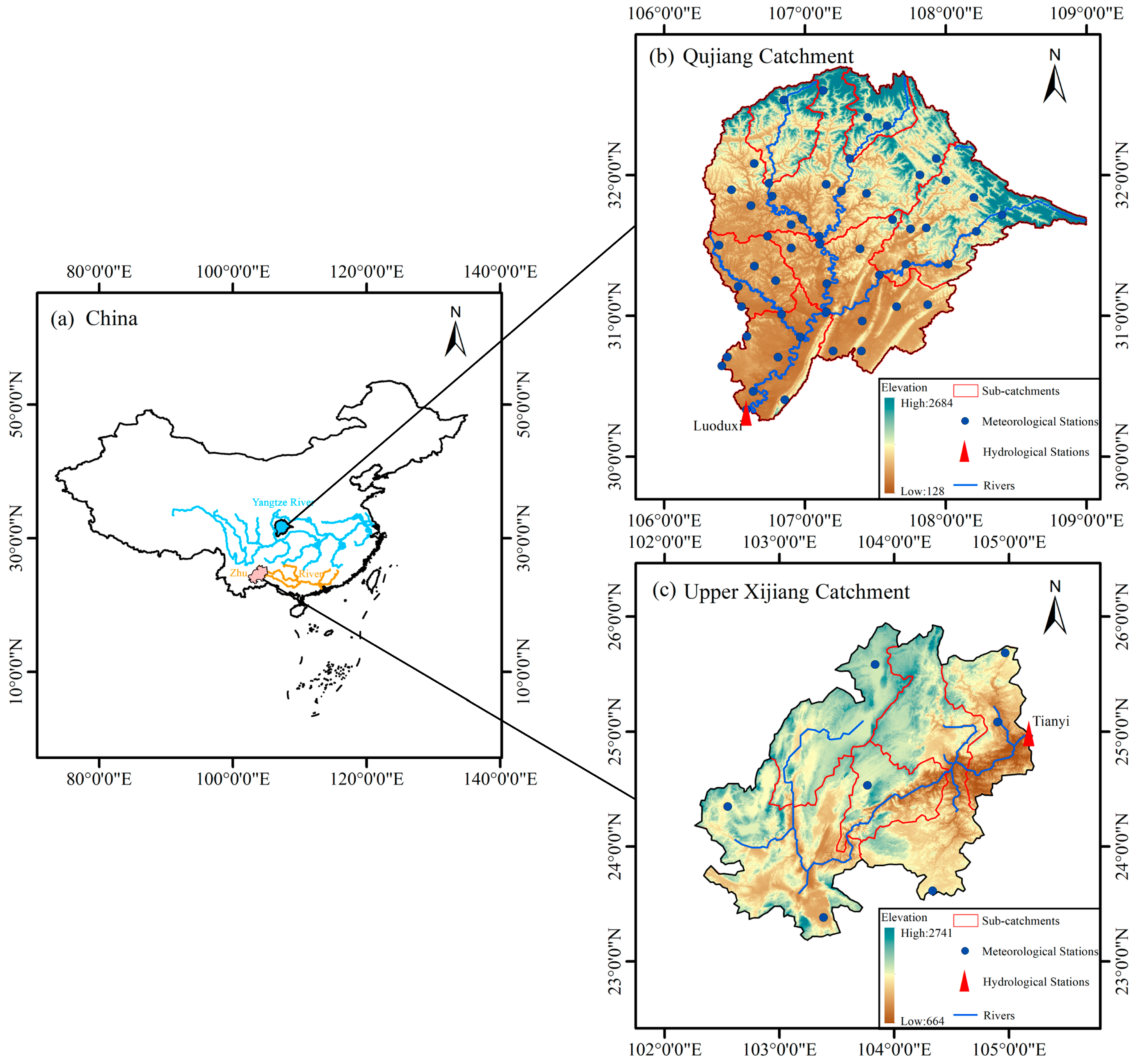
2.1. Study Area

In this study, two typical humid catchments in southwestern China are used for calibration and validation of the distributed hydrological model. These two catchments are both characterized by a subtropical monsoon climate. The Qujiang (QJ) catchment has a drainage area of 39,211 km² (Figure 1a,b). Its elevation ranges from 128 to 2684 m a.s.l.; increasing from southwest to northeast. Its northern part contains the Michang Mountain and the Daba Mountain with low temperature and annual rainfall from 1014 to 1500 mm, while the southern part is plain with relatively moderate temperature covered mostly by the cultivated and dry land. Annual rainfall of the catchment is from 1014 to 1253 mm. Annual mean runoff at the outlet station (Luoduxi station) is 23 billion m³, contributing about thirty percent of the Jialing River’s total discharge. In this study, the Qujiang catchment is divided into seven sub-catchments (circled by red lines in Figure 1b) for modeling, whose sizes are 5513, 7219, 7860, 5264, 6080, 3069, and 4206 km² dividedly from upstream to downstream.

The Upper Xijiang (UXJ) catchment up to the Tianyi reservoir (catchment size 41,715 km²) (Figure 1a,c) belongs to the Zhu River catchment. Its elevation ranges from 664 to 2741 m a.s.l.; increasing from southeast to northwest. The river is originated at the Maxiong Mountain of the Yunnan Province, and the catchment is covered mostly by the forest land with low temperature and annual rainfall from 1200 to 2000 mm. Annual mean runoff at the outlet station (Tianyi station) is 32 billion m³, contributing about ten percent of the Xi River’s total discharge. In this study, the Upper Xijiang catchment is divided into five sub-catchments (circled by red lines in Figure 1c) for modeling, whose sizes are 10,903, 11,850, 5688, 8532, and 4740 km² dividedly from upstream to downstream. For both catchments, the sub-catchments are divided based on river networks.

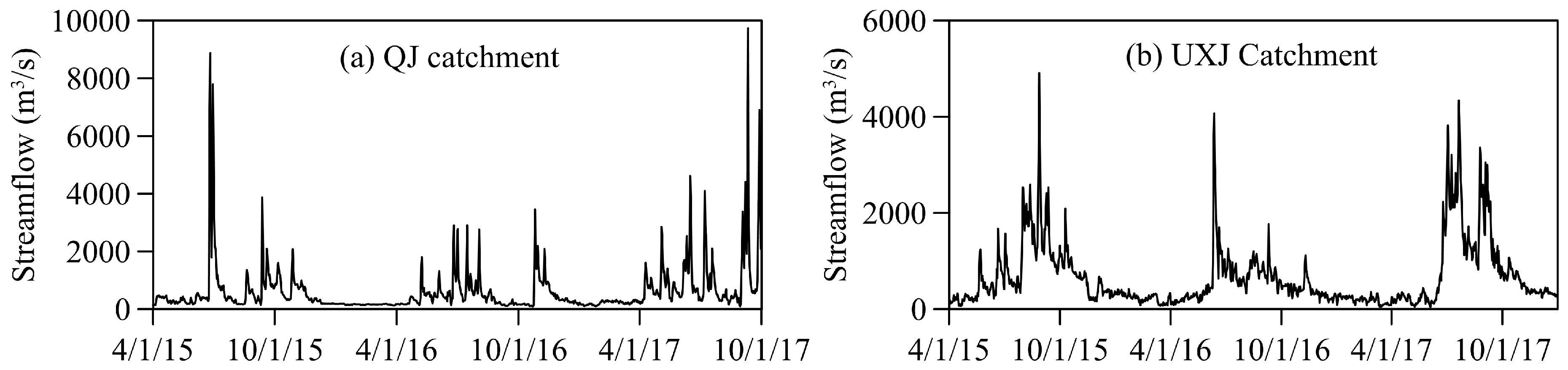
2.2. Hydro-Meteorological Data

In QJ catchment, data used for hydrological modeling include daily meteorological data for 2015.4–2017.9 (precipitation and mean air temperature) from 53 meteorological stations (Figure 1b), and corresponding daily discharge data from the Luoduxi hydrological station (Figure 2a). In UXJ catchment, data used include daily meteorological data for 2015.4–2017.12 from seven meteorological stations (Figure 1c), and corresponding daily discharge data from the Tianyi hydrological station (Figure 2b). The Blaney-Criddle method is used to calculate potential evapotranspiration from mean air temperature data [35]. All input data (precipitation and potential evapotranspiration) are spatially interpolated by the Inverse Distance Weighted (IDW) method with power equaling to two and the maximum radius around 100 km to fit the discrete grids of DEM-based Distributed Rainfall-Runoff Model (DDRM), whose scale is 1 km in this study [36].

2.3. Satellite Soil Moisture Data

Satellite soil moisture data used in this study are acquired from the National Aeronautics and Space Administration’s (NASA) Soil Moisture Active Passive (SMAP) mission. The satellite is the newest L-band soil moisture dedicated satellite in orbit launched on 31 January 2015. It was initially designed to incorporate an L-band (1.41 GHz) passive radiometer and an L-band (1.26 GHz) active radar [7], but its active radar broke down in July 2015. In this study, the SMAP enhanced Level-3 (L3) radiometer global surface soil moisture (SPL3SMP_E) product (version 2), available in the National Snow and Ice Data Center (NSIDC), is chosen [37]. This product is derived based on the Single Channel Algorithm V-pol (SCA-V) [38]. It has a native resolution of around 45 km and is resampled to 9-km resolution. It provides global daily soil moisture contents in m³/m³ within a measuring depth of top 5 cm in the soil profile and covers the period after April 2015.

This SMAP soil moisture product is officially reported with a retrieval uncertainty below 0.04 m³/m³. In recent studies, the quality of different levels of SMAP soil moisture data has been tested by comparing satellite data with field measurements or model simulations worldwide [39,40,41,42,43]. These studies show that in most areas of Europe and America, the overall ubRMSE (unbiased root mean square error) is within the mission requirement. In Qujiang catchment, Xiong et al. (2018) have compared multiple soil moisture datasets, including ASCAT, SMAP, and SMOS soil moisture products [44]. Its result indicates that SMAP product shows reasonable consistency with other datasets. According to Sun et al. (2017)’s study, the ubRMSE of SMAP data in southwest China is 0.055 m³/m³, indicating SMAP soil moisture data capture absolute soil moisture relatively well over southwestern China [42]. In the study, to further identify whether this product is suitable for the two study areas, it also has been compared with a re-analysis dataset, the European Space Agency Climate Change Initiative (ESA CCI) Soil Moisture dataset (version 04.4) (https://www.esa-soilmoisture-cci.org/). Figure 3 indicates that their correlation is high. Thus, SMAP soil moisture product is suitable for the multi-objective calibration in this study. Besides, only the SMAP soil moisture data up to the standard of the Retrieval Quality Flag (RQF) are chosen to screen out data of poor quality, and daily averages of descending and ascending soil moisture estimates in each grid are calculated for calibration.

3. Methodology

Details of methods and procedures are described in this section. The selected distributed rainfall-runoff model is first described, and then the multi-objective Bayesian hierarchical calibration framework is presented to explain how to develop likelihood functions and priors for residual error parameters, followed by a description of data pre-processing. Procedures for calibration and validation are in the last. The graphical summary of procedures for the Bayesian calibration framework is listed in Figure 4.

3.1. The DEM-Based Distributed Hydrological Model

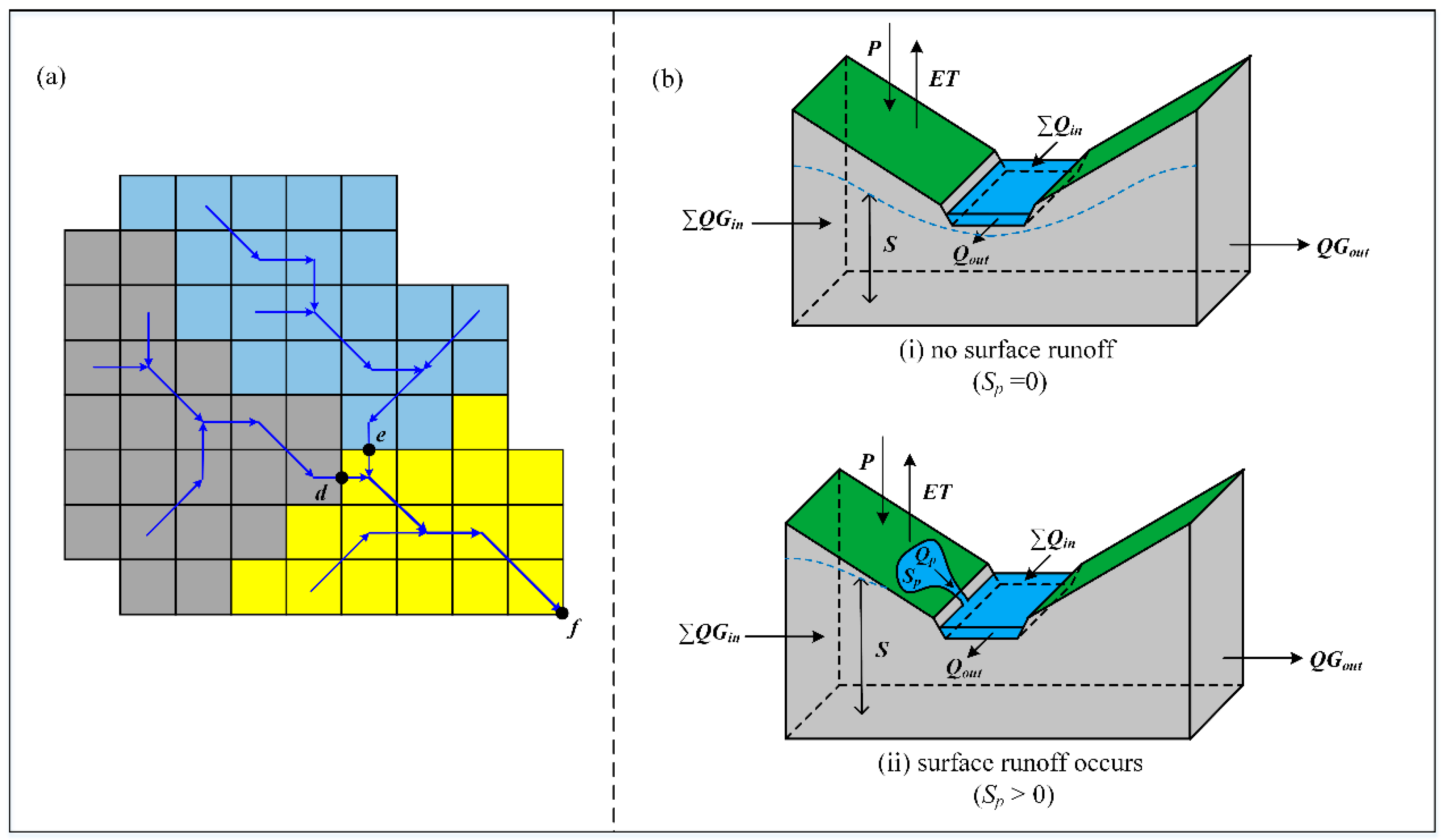
3.1.1. Model Structure

Compared to complex physically-based land-surface models, a conceptual hydrological model, the DEM-based Distributed Rainfall-runoff Model (DDRM) proposed by Xiong et al. (2004), is chosen in the study for its simple model structure with fewer data needed and high efficiency [45]. This model has shown good performances for flood forecasts in humid regions of southern China [44,46,47]. In DDRM, the sub-catchment scheme, which is represented by DEM grids, is used for spatial discretization (Figure 5a). For each DEM grid in the model, soil moisture or other hydrological variables can be simulated. Each sub-catchment outlet is connected to constitute river networks of the whole catchment.

There are three calculation components for the model, including grid excess rainfall calculation, sub-catchment outlet streamflow calculation, and streamflow routing through the river network. Under the saturation excess runoff mechanism, grid excess rainfall calculation is largely influenced by the grid soil water storage capacity ($S_{mc,i}$), which is linked to the corresponding topographic index $\ln \left(\alpha ,\tan \beta \right)$ at the grid $i$. Where soil is unsaturated, there is no excess rainfall generated to replenish the surface ponding water storage. Where soil is saturated, the surface ponding water storage will be replenished and updated (Figure 5b). The grid excess rainfall generation rate is calculated from the surface ponding water storage. Then, the Muskingum method is used to route excess rainfall in each grid from upstream to downstream to get streamflow values at each sub-catchment outlet. This routing method is also used to route streamflow of each sub-catchment to the outlet of the whole catchment but with different parameter schemes. This is because routing streamflow through grids is significantly different from routing streamflow through river networks. In DDRM, grid channel parameters are used when streamflow is routed through grids for inner sub-catchments, and river network routing parameters are used when streamflow is routed through river networks from the sub-catchment outlet to the whole catchment outlet. Thus, streamflow generated in grids in upper reaches of the catchment (grey or blue shaded sub-catchments in Figure 5a) is routed through both grids and river networks, while that generated in grids in lower reaches (yellow shaded sub-catchments in Figure 5a) is routed only through grids. More details of DDRM are shown in Xiong et al. (2018) [44].

The model-simulated soil moisture storage depth $S$ given in mm is the soil moisture output of the distributed model, as shown in Figure 5. It is comparable to the profile soil moisture storage depth. In this study, the scale of DDRM grids is 1 km. To fit 9 km grids for the SMAP soil moisture product, the model-simulated soil moisture storage depth within 1 km is resampled to 9 km, shown as $S_m$ of the grid $m$ (given in mm), and can be converted to the relative saturation ${\phi }_m^{DDRM}$ of the grid $m$ with the grid soil water storage capacity $S_{mc,m}$, which is calculated as:

$${\phi }_m^{DDRM}=\frac{S_m}{S_{mc,m}}$$

(1)

The relative saturation is used for comparison with satellite soil moisture data.

3.1.2. Model Parameters

DDRM is a conceptual distributed model with 11 model parameters, including seven runoff generation parameters ($S_0$, $S_M$, $n$, $a$, $b$, $T_s$, $T_p$), two grid channel routing parameters $c_x\left(x=0,1\right)$, and two river networks routing parameters $h{c}_x^f\left(x=0,1\right)$, among which, $f$ represents different sub-catchments. In this study, only one set of river networks routing parameters is used for all sub-catchments. Before actually moving into model calibration, the sensitivity of model parameters to soil moisture and streamflow has been investigated by local analysis method [48]. Sensitivity indexes are shown in

Table 1. Details of DDRM parameters. Sensitivity indexes $I_{SM}$ and $I_Q$ represent sensitivity to soil moisture and streamflow, respectively. Higher values mean high sensitivity.

Parameter	Unit	Ranges	Description	ISM	IQ
$S_0$	mm	5–100	Minimum water storage capacity	0.01	0.03
$S_M$	mm	5–700	Range of water storage capacity across the catchment	0.10	0.27
$n$	-	0–1	Empirical parameter, reflecting the relationship between $S_{mc,i}$ and corresponding topographic index	0.03	0.15
$a$	-	0–1	Proportion of residual groundwater in soil water storage capacity	0.31	0.29
$b$	-	0–1	Empirical parameter, reflecting the characteristic of ground outflow	0.15	0.03
$T_s$	h	2–200	Time constant, reflecting the characteristic of groundwater	0.07	0.39
$T_p$	h	2–200	Time constant, reflecting the characteristic of surface flow	0	0.01
$c_x\left(x=0,1\right)$	-	0–1	Grid channel parameters of the Muskingum method	0	0.20
$h{c}_x^f\left(x=0,1\right)$	-	0–1	River networks routing parameters of the Muskingum method for sub-catchment $f$	0	0.01

. It indicates that parameters $S_M$, $a$, $b$, and $T_s$ are sensitive to soil moisture, and parameters $S_M$, $n$, $a$, $T_s$, and $c_x\left(x=0,1\right)$ are sensitive to streamflow. More details about DDRM parameters are shown in Table 1.

3.2. Multi-Objective Bayesian Hierarchical Framework

A multi-objective Bayesian calibration framework, which both considers the trade-off between objectives and undertakes the model uncertainty analysis, is recommended in this study. To satisfy the spatial and temporal heteroscedasticity of distributed model residuals, heteroscedastic residual error models with unknown parameters that link residual variances with hydrological covariates are used in likelihood functions. Details of the multi-objective Bayesian hierarchical framework are presented below.

3.2.1. Multi-Objective Likelihood Function

Simulations of conceptual hydrological models systematically deviate from observations, and a conceptual distributed hydrological model can be expressed as:

$$Y_{m,t}=y_{m,t}\left(X,\theta \right)+{\epsilon }_{m,t}^Y$$

(2)

It is assumed that the system response at the time $t$ of each grid $m$ of the distributed model can be represented by a deterministic function $y_{m,t}\left(X,\theta \right)$, where $X$ is the input of models and $\theta$ is a hydrological model parameter. $Y_{m,t}$ is the observation at the time $t$ of the grid $m$, and ${\epsilon }_{m,t}^Y$ is the corresponding residual term. In this study, observed streamflow at the catchment outlet $Q_t$ and gridded soil moisture $S{M}_{m,t}$ can be expressed as:

$$Q_t=q_t\left(X,\theta \right)+{\epsilon }_t^Q$$

(3)

$$S{M}_{m,t}=s{m}_{m,t}\left(X,\theta \right)+{\epsilon }_{m,t}^{SM}$$

(4)

where $q_t\left(X,\theta \right)$ denotes simulated streamflow at the catchment outlet, and $s{m}_{m,t}\left(X,\theta \right)$ denotes simulated gridded soil moisture of the distributed model. ${\epsilon }_t^Q$ and ${\epsilon }_{m,t}^{SM}$ represent corresponding residual terms for Q and SM, respectively. In the Bayesian framework, posterior distributions of unknown model parameters can be calculated as:

$$P\left(\theta |Q_t,S{M}_{m,t}\right)=\frac{P\left(\theta \right)\cdot P\left(Q_t,S{M}_{m,t}|\theta \right)}{P\left(Q_t,S{M}_{m,t}\right)}\propto P\left(\theta \right)L\left(\theta |Q_t,S{M}_{m,t}\right)$$

(5)

$P\left(\theta \right)$ denotes the prior information of hydrological model parameters, and $L\left(\theta |Q_t,S{M}_{m,t}\right)\equiv P(Q_t,S{M}_{m,t}|\theta )$ denotes the likelihood function. For numerical stability, log-likelihood functions are usually used instead of likelihood functions [30,49]. If the residual terms are assumed to be normally distributed, uncorrelated with variance varying in time and space, the log-likelihood function for multi-objective distributed model calibration can be written as:

$$L_Q=-\frac{T}{2}\ln \left(2\pi \right)-{\displaystyle \sum _{t=1}^T\ln \left[{\sigma }_t^{{\epsilon }^Q}\right]}-\frac{1}{2}{\displaystyle \sum _{t=1}^T\frac{{\left({\epsilon }_t^Q\right)}^2}{{\left({\sigma }_t^{{\epsilon }^Q}\right)}^2}}$$

(6)

$$L_{SM}=-\frac{T}{2}\ln \left(2\pi \right)-\frac{1}{M}{\displaystyle \sum _{t=1}^T{\displaystyle \sum _{m=1}^M\ln \left[{\sigma }_{m,t}^{{\epsilon }^{SM}}\right]}}-\frac{1}{2M}{\displaystyle \sum _{t=1}^T{\displaystyle \sum _{m=1}^M\frac{{\left({\epsilon }_{m,t}^{SM}\right)}^2}{{\left({\sigma }_{m,t}^{{\epsilon }^{SM}}\right)}^2}}}$$

(7)

$$L_{multi}=L_Q+L_{SM}$$

(8)

where ${\sigma }_t^{{\epsilon }^Q}$ represents the individual streamflow error standard deviation at the time $t$, and ${\sigma }_{m,t}^{{\epsilon }^{SM}}$ represents the individual soil moisture error standard deviation at the time $t$ of grid $m$.

To satisfy the heteroscedasticity nature of distributed model residuals, an advanced heteroscedastic error model is constructed. This heteroscedastic error model contains unknown parameters of model residuals, assuming residual variances to be related to hydrological covariates that vary in time and space. These residual error models with unknown parameters that simulated through calibration have their advantages in assuming residual errors as a mixture of errors from the model structure and observations [49].

In practice, suitable covariates are selected from various candidate explanatory variables that include observed streamflow, satellite soil moisture, and antecedent precipitation. It is performed by using the Generalized Additive Models for Location, Scale, and Shape (GAMLSS) method with Akaike’s information criterion (AIC) [50,51]. Good residual error models are shown as followed.

The residual error model for streamflow uses seven-day catchment-averaged antecedent precipitation $P_t^{7ant}$ as the covariate, which can be written as:

$$\mathrm{l}\mathrm{n}\left[{\sigma }_t^{{\epsilon }^Q}\right]={\psi }_0^Q+{\psi }_1^Q\cdot P_t^{7ant}$$

(9)

The residual error model for soil moisture uses five-day gridded antecedent precipitation $P_{m,t}^{5ant}$ of grid $m$ as the covariate, which can be written as:

$$\ln \left[{\sigma }_{m,t}^{{\epsilon }^{SM}}\right]={\psi }_0^{SM}+{\psi }_1^{SM}\cdot P_{m,t}^{5ant}$$

(10)

where ${\psi }_0^Q$, ${\psi }_1^Q$, ${\psi }_0^{SM}$, and ${\psi }_1^{SM}$ are hierarchical error model parameters.

3.2.2. Prior Information

It is essential to construct appropriate prior distributions of parameters to calculate their posterior distributions when data are limited. Priors of hydrological model parameters are normally set to be uniformly distributed among their psychically accepted ranges (Table 1), while priors of residual error model parameters for multi-objective calibration need to be constructed following two guidelines. Firstly, values of residual variances can substitute for weights of objectives prescribed in traditional multi-objective calibration. For one objective among multiple objectives, a smaller variance means more emphasis on this objective. Secondly, modeled residuals should be in accepted ranges. In this study, priors for residual error model parameters are developed based on a Pareto-based multi-objective method to satisfy the two guidelines. The Pareto front from the Pareto-based method demonstrates the trade-off between objectives on optimizing streamflow and soil moisture. Different Pareto points in the Pareto front can be used to represent different weights of the two objectives. Priors for residual error model parameters are constructed as normal distributions with means calculated based on corresponding residual time series of the selected Pareto point in the Pareto front by GAMLSS, and variances of priors are defined on the basis of the magnitude of means (Figure 2). This is because the values of these means are the key to constrict the two objectives, and the exact values of variances for priors are less influential in this Bayesian framework [30,52].

3.3. Pre-Processing for Calibration Data

Obviously, satellite surface soil moisture is not comparable to profile soil moisture simulated by the chosen distributed model with one soil layer [53]. Two ways can be used to solve the problem: (i) configuring the distributed hydrological model to simulate surface soil moisture at an observed depth; (ii) converting satellite surface soil moisture to soil water index that can be comparable to the profile soil moisture. For the first way, more data, such as vegetation types and soil types, and more complex model structure and more parameters are needed to introduce to the model. Since the aim of the study is to identify the value of satellite data in calibrating a distributed model, but not to investigate how to improve the model structure for better matching model-simulate soil moisture to satellite soil moisture, the model structure remains, and the second way is chosen.

A method named the Exponential Filter proposed by Wagner et al. (1999) is used to convert satellite surface soil moisture to soil water index [54]. Previous studies have used soil water index to calibrate hydrological models [19,22]. In this study, for each grid $m$ of SPL3SMP_E product, surface soil moisture content ${\omega }_{SSM}^{L3}\left(m,t_n\right)$ (given in m³/m³) is converted to soil water index ${\omega }_{SWI}^{L3}\left(m,t_n\right)$ based on the assumption that time variation of profile soil moisture is linearly related to the difference between surface soil moisture and profile soil moisture. Thus,

$${\omega }_{SWI}^{L3}\left(m,t_n\right)={\omega }_{SWI}^{L3}\left(m,t_{n-1}\right)+K_n\left[{\omega }_{SSM}^{L3}\left(m,t_n\right)-{\omega }_{SWI}^{L3}\left(m,t_{n-1}\right)\right]$$

(11)

where time $t_n$ indicates acquisition time of ${\omega }_{SSM}^{L3}$, and $t_{n-1}$ indicates previous acquisition time. $K_n$ is the gain term at the time $t_n$. It varies between 0 and 1 as follows,

$$K_n=\frac{K_{n-1}}{K_{n-1}+e^{-\left(\frac{t_n-t_{n-1}}{CT}\right)}}$$

(12)

For initialization of the filter, $K_1$ is set to 1. $CT$ is the Characteristic Time length representing timescale of soil moisture variation to obtain profile soil moisture. In the study, the value of $CT$ is calculated by maximizing the correlation between exponentially filtered profile soil moisture and model-simulated soil moisture by a simple calibration from the range of 5 days to 55 days. $CT$ equaling to 25 days and 20 days are chosen, respectively, for QJ catchment and UXJ catchment, which are similar to 20 days used in the study of Xiong et al. (2018). The value below or above the chosen value for each catchment gets the worse correlation. Then, ${\omega }_{SWI}^{L3}\left(m,t_n\right)$ of each grid $m$ given in m³/m³ is converted to relative saturation ${\phi }^{L3}\left(m,t_n\right)$. For a long time series $T_l$ in each grid $m$ of the SMAP soil moisture product, the value of the maximal soil moisture content can be regarded as the soil porosity value. Thus, the minimum-maximum correction method can be used as:

$${\phi }^{L3}\left(m,t_n\right)=\frac{{\omega }_{SWI}^{L3}\left(m,t_n\right)-\underset{T_l}{{\displaystyle \min }}\left[{\omega }_{SWI}^{L3}\left(m,T_l\right)\right]}{\underset{T_l}{{\displaystyle \max }}\left[{\omega }_{SWI}^{L3}\left(m,T_l\right)\right]-\underset{T_l}{{\displaystyle \min }}\left[{\omega }_{SWI}^{L3}\left(m,T_l\right)\right]}$$

(13)

Since soil moisture derived from DDRM and soil water index derived from SPL3SMP_E are all converted to relative saturation, these soil moisture simulations are comparable. In this study, gridded ${\phi }^{L3}\left(m,t_n\right)$ is used for calibration, shown as L3SWI.

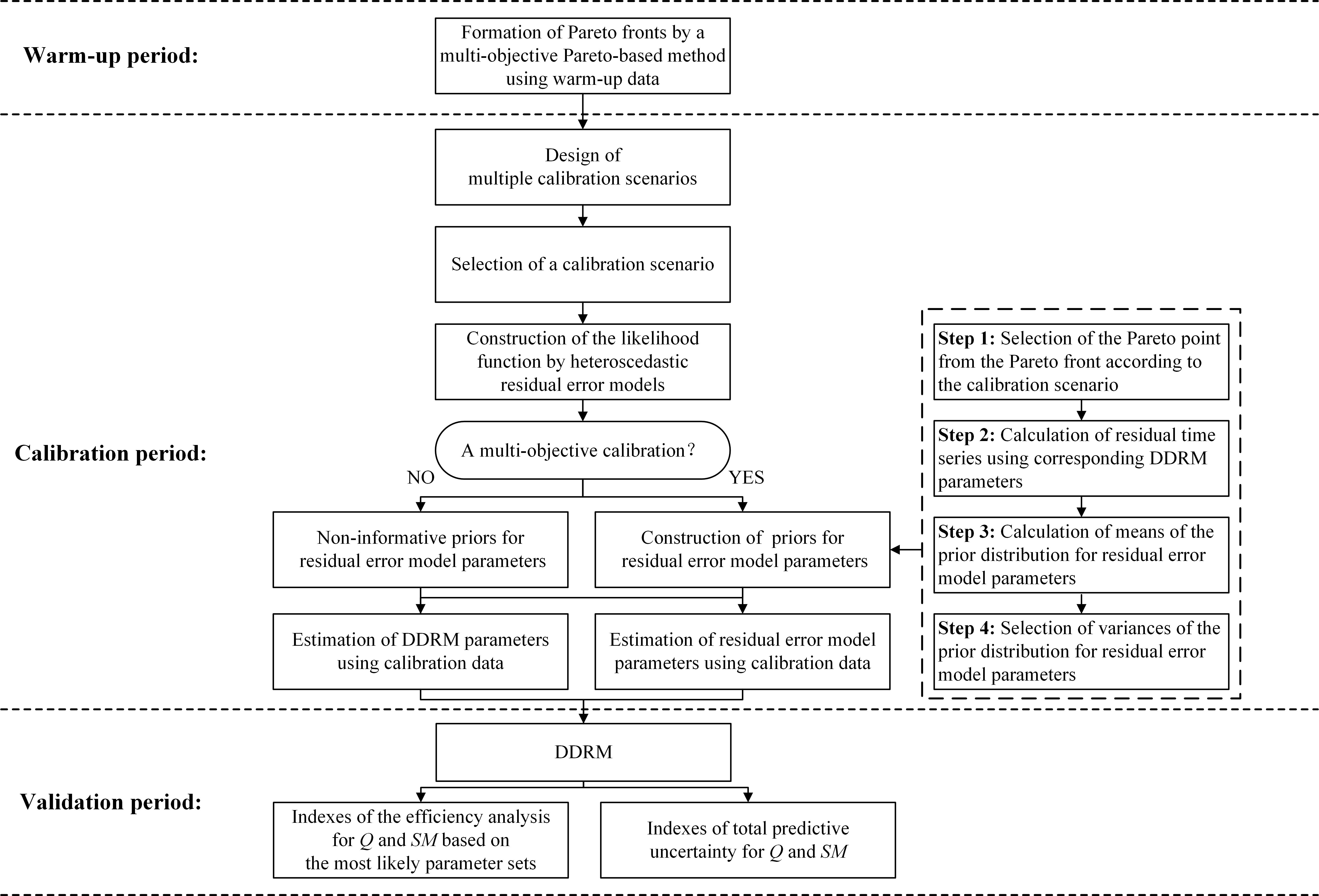
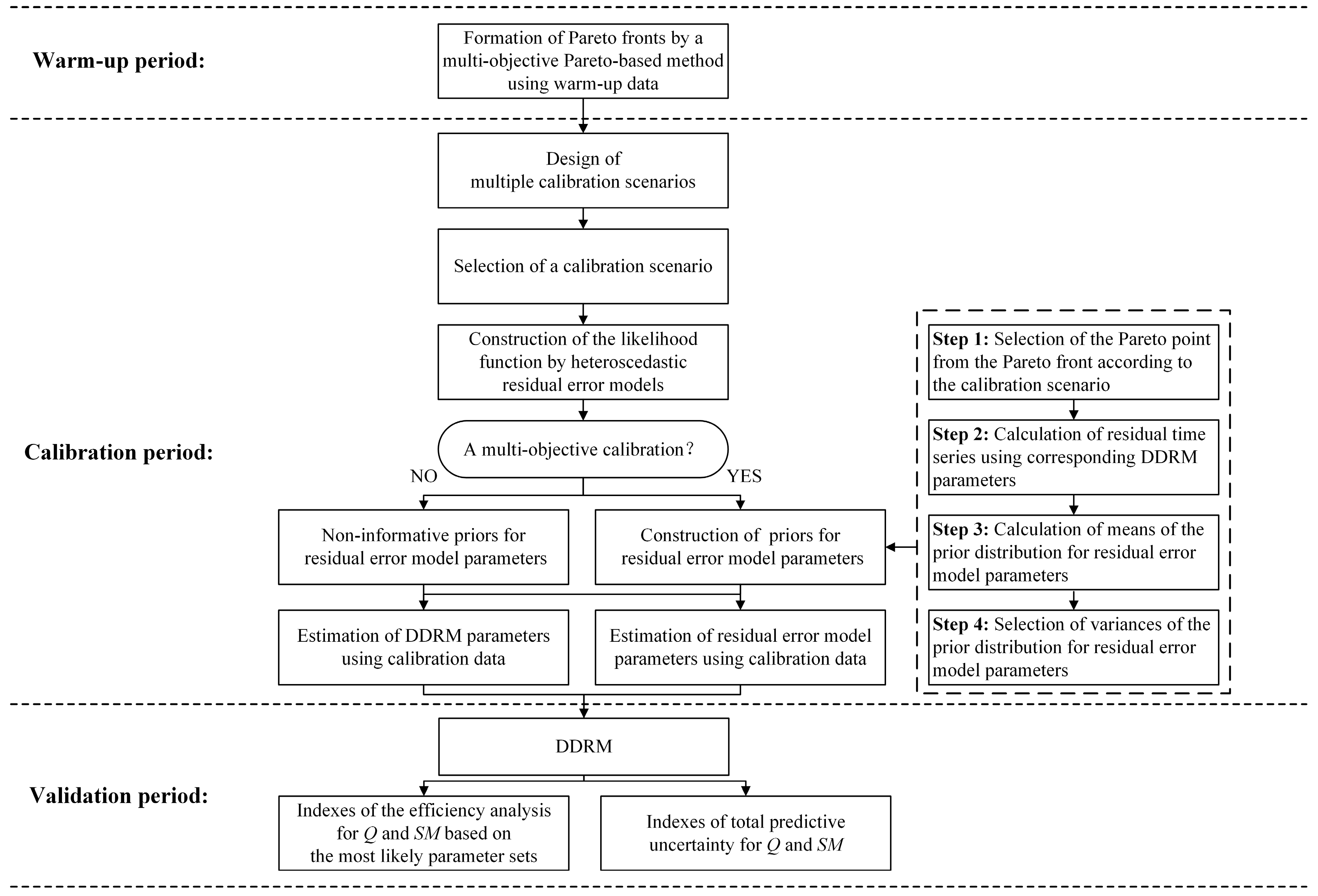
3.4. Procedures for Calibration and Validation

Procedures for the Bayesian hierarchical calibration framework are listed in Figure 4. The whole period is divided into the warm-up period, the calibration period, and the validation period (

Table 2. Periods for warm-up, calibration, and validation for Qujiang and Upper Xijiang catchments.

Catchment	Warm-up Period	Calibration Period	Validation Period
Qujiang	April 2015–September 2015	October 2015–March 2017	April 2017–September 2017
Upper Xijiang	April 2015–September 2015	October 2015–May 2017	June 2017–December 2017

). Data before 01 October 2015 are used for the warm-up period to form Pareto fronts between the two objectives for both catchments. In this study, AMALGAM is used to acquire the Pareto front of the Kling-Gupta Efficiency ($KGE$) of streamflow and soil moisture using warm-up data [55]. In the simulation, 100 generations and 100 populations are defined. Through the selection of different Pareto points in the Pareto front, multiple multi-objective calibration scenarios are designed for each catchment. Simultaneously, the streamflow-based single objective calibration is designed as the benchmark, and the soil moisture-based single objective calibration is designed only as supplementary information. In the calibration period, non-informative priors for residual error model parameters are used for single objective scenarios, and informational priors constructed based on the selected Pareto points are used for multi-objective scenarios. For each of the Bayesian calibration scenario, the DREAM algorithm is employed to calculate posterior distributions of a hydrological model and residual error model parameters. Eight Markov chains and 10,000 generations are defined, and for each Markov chain, generations for which the $\stackrel{\wedge }{R}$ statistics of convergence diagnostics are below the critical threshold 1.2 for all parameters are selected for the target distribution.

After the estimation of hydrological model and residual error model parameters, summary statistics of model simulations acquired based on the most likely parameter values are calculated for the efficiency analysis in both calibration and validation periods, among which, the Kling-Gupta Efficiency ($KGE$) and its components ($G1$, $G2$, and $G3$) are calculated separately for streamflow simulations, while $KGE$, the Residual error ($RE$), Lin’s Concordance Correlation Coefficient ($CCC$), and the Root Mean Square Error ($RMSE$) are used for soil moisture simulations [15,18,55,56]. In the meanwhile, 90% confidence limits of total predictive uncertainties for Q and SM are also calculated, respectively, for each catchment [30]. Ninety percent confidence limits of total predictive uncertainty are calculated by adding to model simulations a random noise drawn from a normal distribution with mean 0 and the time-varying or space-varying variance, which is computed by Equation (9) or Equation (10). For single objective scenarios, since the residual variance for Q cannot be acquired from Equation (9) in S2, and the residual variance for SM cannot be acquired from Equation (10) in S1, these variances are substituted by the mean square error between observations and simulations. To clearly illustrate the uncertainty, summary statistics proposed in Xiong et al. (2009), including the Containing Ratio ($CR$), the Average Bandwidth ($B$), and the Average Deviation Amplitude ($D$), are considered [57]. Higher values of $CR$ and lower values of $B$ indicate better performances, but higher values of $CR$ and higher values of $B$ are more likely to appear simultaneously. Thus, in this study, the Transformed Average Bandwidth ($TB$) is substituted for $B$, which is calculated as $TB=B/CR$. All results are compared and analyzed.

4. Results and Discussion

4.1. Prior Information for Residual Error Model Parameters

Prior distributions for residual error model parameters are constructed by the Pareto front. The Pareto front of $KGE$ between observed and model-simulated streamflow (x-axis) and that between pre-processed satellite and model-simulated soil moisture (y-axis) for each catchment is shown in Figure 6. Points in each of the Pareto fronts present a clear trade-off between two objectives. For each objective, the larger $KGE$ means more emphasis on the objective. In both chosen catchments, values of $KGE$ for streamflow distribute in larger ranges (35% to 75% in QJ catchment, 40% to 80% in UXJ catchment) than those for soil moisture (41% to 50% in QJ catchment, 54% to 63% in UXJ catchment). It indicates that weights of soil moisture in multi-objective calibration largely influence the performance of streamflow simulations. Besides, the Pareto front in UXJ catchment gets better performance than that in QJ catchment, either for streamflow and soil moisture.

For each Pareto front, points representing the least $KGE$ of Q (the least emphasis on streamflow), the middle one (the middle emphasis on streamflow), and the largest $KGE$ of Q (the largest emphasis on streamflow) are selected to construct priors for multi-objective calibration scenarios, signed as M1–M3 for each catchment. Meanwhile, single objective calibration scenarios, signing as S1 (Q only), S2 (L3SWI only), respectively, are chosen for comparisons in each catchment. In this study, all prior distributions of hierarchical error parameters are transformed to get the means that are of the same magnitude, and their values of variances are defined as 0.02. Priors of residual error parameters in different scenarios are shown in

Table 3. Prior distributions of heteroscedastic residual error parameters (${\psi }_0^Q$, ${\psi }_1^Q$, ${\psi }_0^{SM}$, and ${\psi }_1^{SM}$) in various Bayesian scenarios (S1–S2, M1–M3) in either Qujiang (QJ) catchment and Upper Xijiang (UXJ) catchment.

Catchment	Scenario	${\mathit{\psi }}_0^{\mathit{Q}}$	${\mathit{\psi }}_1^{\mathit{Q}}*100$	${\mathit{\psi }}_0^{\mathit{S}\mathit{M}}$	${\mathit{\psi }}_1^{\mathit{S}\mathit{M}}*1000$
QJ	S1	$Unif\left(3,6\right)$	$Unif\left(1,3\right)$	-	-
	S2	-	-	$Unif\left(-4,0\right)$	$Unif\left(-3,10\right)$
	M1	$Norm\left(5.25,0.02\right)$	$Norm\left(2.26,0.02\right)$	$Norm\left(-2.70,0.02\right)$	$Norm\left(2.28,0.02\right)$
	M2	$Norm\left(5.26,0.02\right)$	$Norm\left(2.04,0.02\right)$	$Norm\left(-2.74,0.02\right)$	$Norm\left(3.61,0.02\right)$
	M3	$Norm\left(5.28,0.02\right)$	$Norm\left(1.83,0.02\right)$	$Norm\left(-2.34,0.02\right)$	$Norm\left(-2.63,0.02\right)$
UXJ	S1	$Unif\left(3,6\right)$	$Unif\left(1,3\right)$	-	-
	S2	-	-	$Unif\left(-4,0\right)$	$Unif\left(-3,10\right)$
	M1	$Norm\left(5.56,0.02\right)$	$Norm\left(1.22,0.02\right)$	$Norm\left(-1.76,0.02\right)$	$Norm\left(-2.74,0.02\right)$
	M2	$Norm\left(5.44,0.02\right)$	$Norm\left(1.02,0.02\right)$	$Norm\left(-1.75,0.02\right)$	$Norm\left(-2.73,0.02\right)$
	M3	$Norm\left(5.14,0.02\right)$	$Norm\left(1.25,0.02\right)$	$Norm\left(-1.72,0.02\right)$	$Norm\left(-2.34,0.02\right)$

.

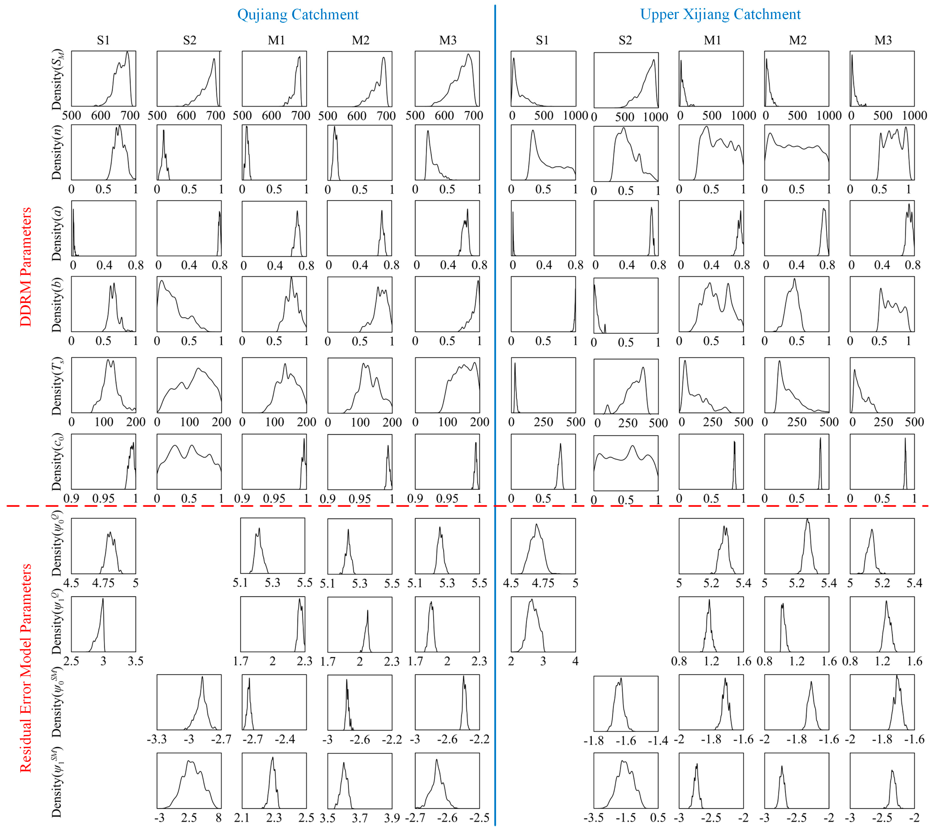
4.2. Posterior Information for Parameters

Figure 7 illustrates posterior distributions for DDRM parameters with high sensitivity to soil moisture or streamflow (the first six rows) and residual error model parameters (the last four rows) for QJ and UXJ catchments. It can be seen that for each catchment, posterior distributions for most parameters (except parameter $C_0$) in scenarios M1–M3 seem to be combinations of those in the scenarios S1 and S2, indicating these parameters are affected by both soil moisture and streamflow. Parameters $S_M$, $n$, and $T_s$ are more sensitive to streamflow, and there is a trend in their posterior distributions to be more similar to the scenario S1 from the scenario M1 to the scenario M3. Parameters $a$ and $b$ are more sensitive to soil moisture, their posterior distributions in the scenario M1 are more similar to those in the scenario S2 than in M2 and M3. Parameter $C_0$ is nearly not affected by soil moisture. The results are quite consistent with what the sensitivity of each parameter shows in Table 1. In the scenario S2, parameters $T_s$ and $C_0$ are relatively diffuse, indicating these parameters have not been well calibrated. Besides, there is an obvious discrepancy between posterior distributions of most parameters in the scenario S1 and the scenario S2 for both catchments. It indicates the large parameter uncertainty in the single-objective calibration.

The last four rows of Figure 7 show posterior distributions of residual error model parameters. They can represent the fitness between simulations and observations since a smaller residual variance means a better model performance. Differences between their prior and posterior distributions are significant in single objective calibration scenarios, but posterior distributions in multi-objective scenarios show only a slight shift to their priors (Table 3). This is because single objective scenarios set large ranges for these parameters, while multi-objective calibration scenarios set narrow ranges since priors for these parameters are used as constraints for model residuals. It indicates that priors of hierarchical error parameters have a great influence on their posterior distributions, and this is similar to the results of Yating et al. (2018) [30]. Thus, it is reasonable to weight different objectives by defining different priors in multi-objective Bayesian calibration.

4.3. Observed and Model-Simulated Daily Streamflow and Soil Moisture Data

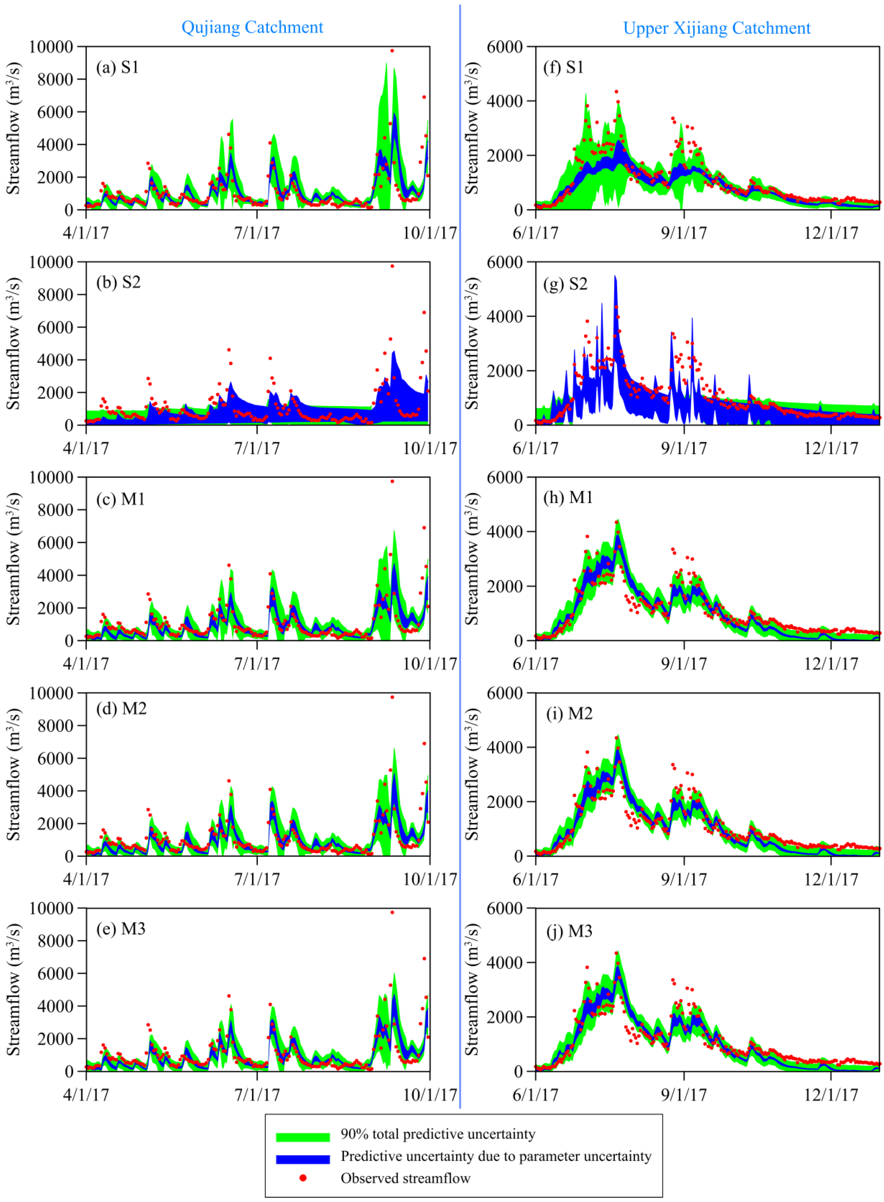
4.3.1. Observed and Model-Simulated Daily Streamflow

Table 4. Indexes for the efficiency analysis of model-simulated Q that is calculated with the most likely parameter values, including the Kling-Gupta Efficiency $KGE$(%) and its components $G1$(%), $G2$(%), and $G3$(%), and indexes for 90% confidence limits of total predictive uncertainty for Q (m³/s), including the Containing Ratio $CR$(%), the Transformed Average Bandwidth $TB$(m³/s), and the Average Deviation Amplitude $D$(m³/s) for multiple scenarios (single objective S1–S2, multi-objective M1–M3) in calibration and validation periods for the Qujiang catchment and the Upper Xijiang catchment.

		Qujiang Catchment						Upper Xijiang Catchment
	Index	S1	S2	M1	M2	M3		S1	S2	M1	M2	M3
Calibration period	$KGE$	71.25	–24.79	57.32	65.04	71.57		57.22	13.05	72.52	79.52	81.70
	$G1$	2.31	75.62	5.33	3.62	2.59		2.84	6.51	2.82	1.28	1.38
	$G2$	5.49	50.71	7.77	5.28	3.52		11.41	38.25	0.41	0.39	0.18
	$G3$	0.46	29.36	5.11	3.32	1.97		4.05	30.85	4.32	2.52	1.79
	$CR$	90.35	94.72	90.53	89.79	90.89		85.37	85.37	77.55	82.72	84.74
	$TB$	610.01	1004.85	658.74	636.90	622.49		676.35	897.48	644.94	643.59	639.08
	$D$	128.64	257.07	122.47	125.15	121.96		157.15	245.24	151.31	146.90	146.67
Validation period	$KGE$	70.10	–23.48	52.73	59.60	65.90		56.79	16.81	77.90	82.90	84.77
	$G1$	2.68	67.65	5.96	4.35	3.35		1.88	4.78	1.88	0.93	0.99
	$G2$	5.81	53.52	9.43	6.89	5.16		12.09	33.65	0.01	0.05	1.02
	$G3$	0.47	31.30	6.95	5.07	3.11		4.70	30.77	2.98	1.94	0.01
	$CR$	80.01	69.40	74.87	77.59	80.24		77.46	66.20	58.22	60.09	63.38
	$TB$	1806.81	1611.26	1754.37	1649.91	1569.45		1260.93	1363.79	1176.83	1168.31	1159.15
	$D$	412.97	580.35	407.90	407.59	396.64		345.76	511.94	298.76	297.53	296.20

illustrates summary statistics for the efficiency analysis of Q calculated based on the most likely parameter values and summary statistics for 90% confidence limits of total predictive uncertainty for Q in both calibration and validation periods. It indicates that performances of streamflow simulations are different in Qujiang and Upper Xijiang catchment when adding satellite soil moisture data. In Qujiang catchment, the efficiency analysis shows that adding satellite soil moisture data in model calibration is not beneficial to performances of streamflow simulations, and the uncertainty analysis shows that it can reduce streamflow uncertainty, especially in the validation period. However, in Upper Xijiang catchment, the benefits of satellite data are quite obvious. Adding satellite soil moisture data has a positive influence on streamflow simulations for Upper Xijiang catchment according to both efficiency analysis and uncertainty analysis. The worse efficiency of streamflow simulations in multi-objective scenarios of Qujiang catchment may due to nonstationarity in annual streamflow (Figure 2). Overall, one conclusion can be inferred that adding soil moisture data as constraints for calibration can reduce uncertainty in streamflow simulations. As for different multi-objective calibration scenarios, it can be observed that streamflow simulations perform better in scenarios where more emphasis is put on streamflow in both catchments.

Figure 8 demonstrates ranges of 90% confidence limits of total predictive uncertainty and the predictive uncertainty due to the parameter uncertainty in daily streamflow during the validation period in QJ and UXJ catchments. It can be seen that the predictive uncertainty due to the parameter uncertainty in scenarios S2 is much worse than other scenarios. It means poor parameter estimates are acquired for streamflow, and thus result in poor total predictive uncertainty. It indicates that the application of satellite soil moisture on simulating streamflow by conceptual hydrological models in ungauged areas still remains problematic, although values of satellite soil moisture in ungauged areas were identified for some complex parametrized physically-based land-surface models [58]. For each catchment, multi-objective scenarios show similar patterns, and predictive streamflow follows the fast fluctuations of observed streamflow. The visible difference is that 90% confidence limits of total predictive uncertainty in scenarios S1 cover more high-flow points than other scenarios in each catchment, indicating that predictive streamflow in scenarios S1 can better simulate high flow. For all scenarios, some points are still not covered by the predictive uncertainty. This may due to that a simple linear residual error model can only partly satisfy residual heteroscedasticity.

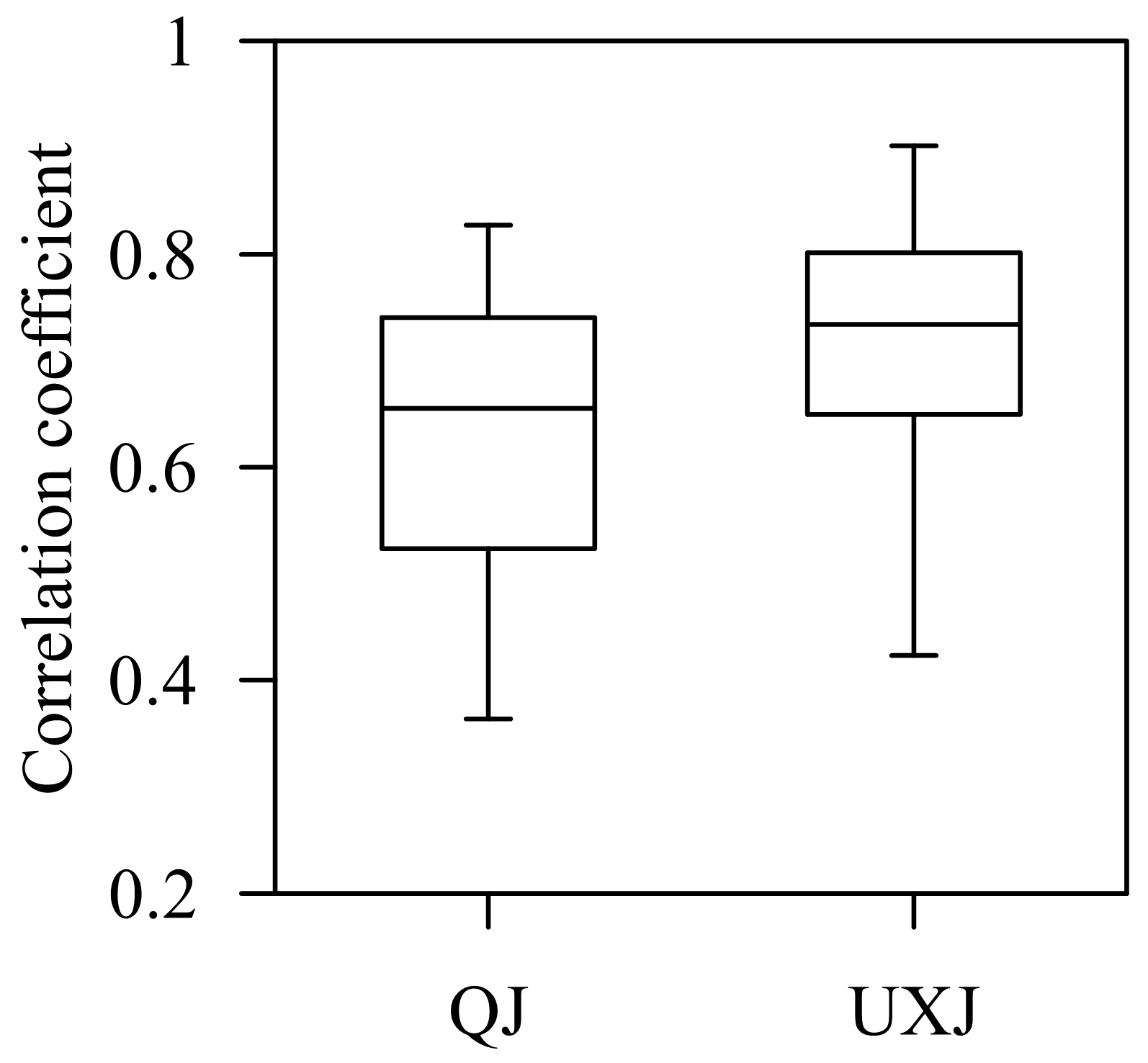
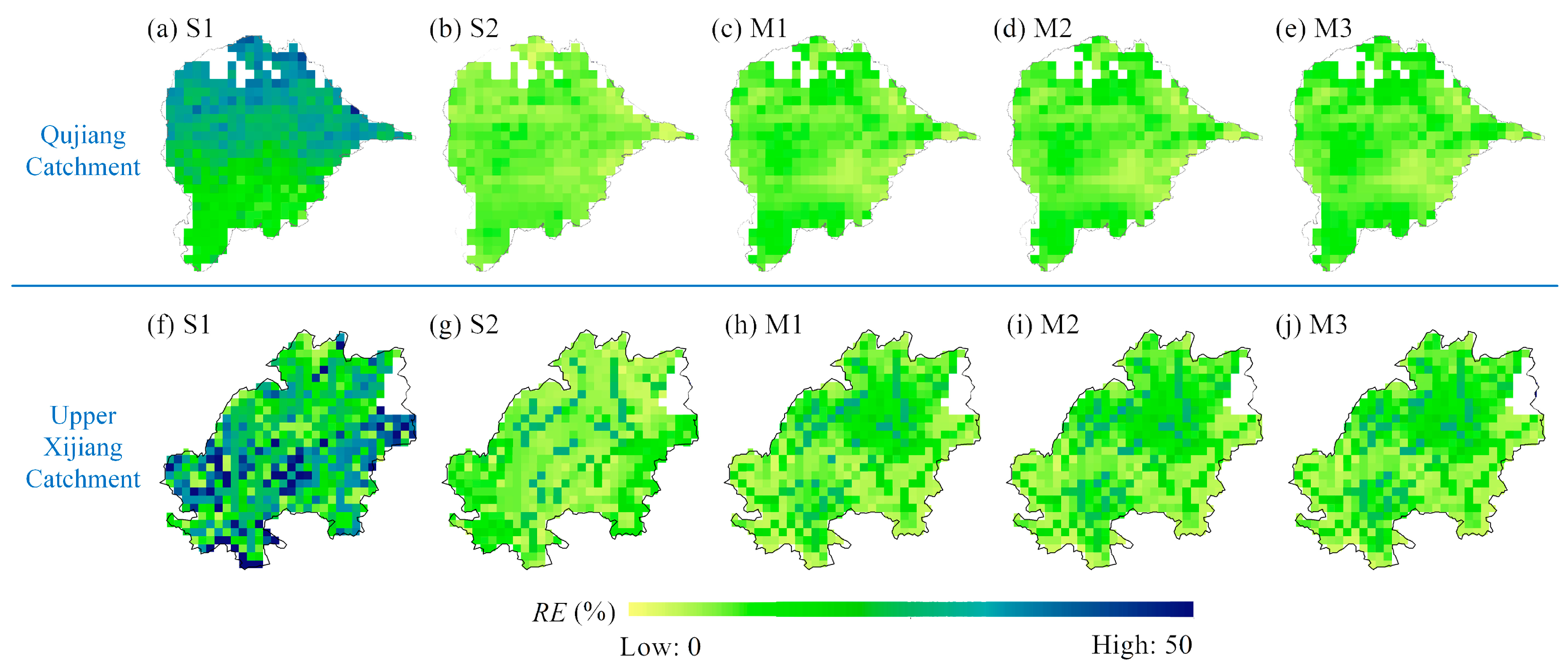
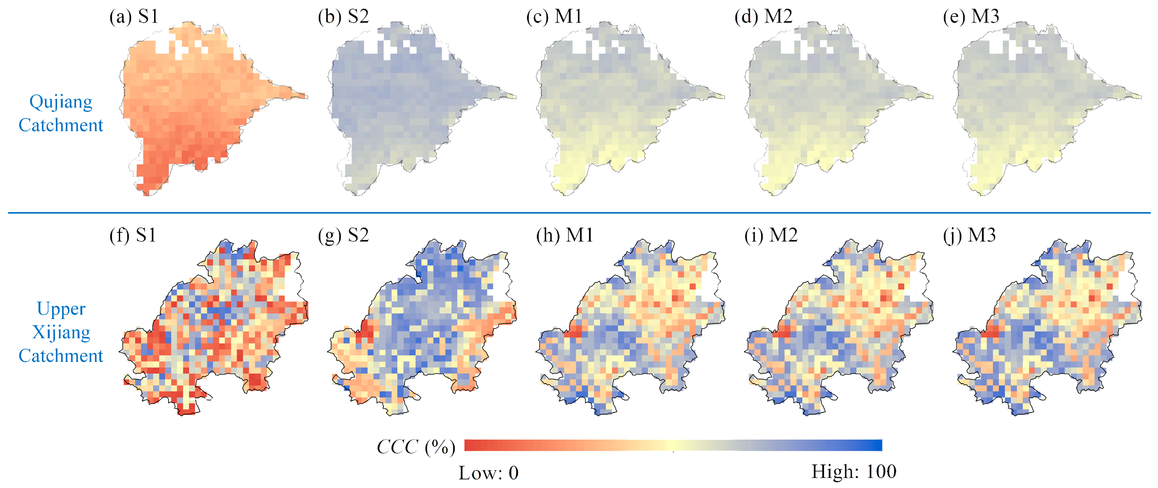
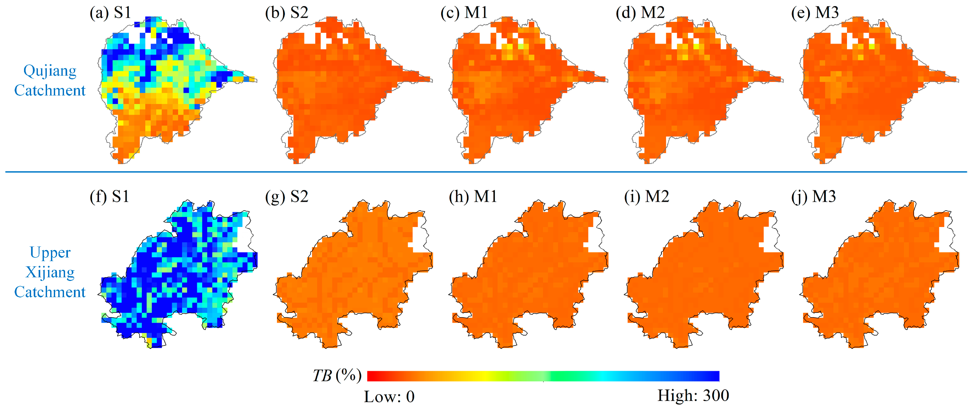
4.3.2. Observed and Model-Simulated Daily Soil Moisture

Table 5. Catchment-averaged indexes for the efficiency analysis of model-simulated gridded SM that is calculated with the most likely parameter values, including the Kling-Gupta Efficiency $KGE$ (%), the Residual Error $RE$ (%), Lin’s Concordance Correlation Coefficient $CCC$ (%), and the Root Mean Squared Error $RMSE$ (%), and indexes for 90% confidence limits of total predictive uncertainty for gridded SM (%), including the Containing Ratio $CR$ (%), the Transformed Average Bandwidth $TB$ (%), and the Average Deviation Amplitude $D$ (%) for multiple scenarios (single objective S1–S2, multi-objective M1–M3) in calibration and validation periods for both Qujiang and Upper Xijiang catchments.

		Qujiang Catchment						Upper Xijiang Catchment
	Index	S1	S2	M1	M2	M3		S1	S2	M1	M2	M3
Calibration period	$KGE$	–142.17	33.63	31.22	31.11	27.40		–0.95	42.32	45.07	43.56	44.21
	$RE$	31.30	7.74	8.91	8.93	9.56		33.40	9.89	8.74	8.89	9.05
	$CCC$	28.64	59.95	52.48	51.32	50.25		25.13	55.69	69.57	70.47	68.97
	$RMSE$	32.81	9.04	10.17	10.19	10.82		32.92	8.62	7.99	8.10	8.23
	$CR$	12.08	79.87	79.35	79.44	87.30		11.36	73.88	67.48	67.66	67.68
	$TB$	687.38	23.82	28.93	29.13	32.00		589.56	26.93	28.33	29.15	29.99
	$D$	29.66	5.42	6.68	6.72	7.59		21.33	5.93	6.87	7.09	7.15
Validation period	$KGE$	–119.05	36.74	36.00	35.89	32.94		6.58	45.62	46.74	48.35	46.68
	$RE$	20.29	9.30	10.06	10.05	10.37		24.25	8.72	10.02	10.47	10.51
	$CCC$	23.76	63.18	56.37	55.44	54.42		36.86	64.14	58.07	58.10	61.17
	$RMSE$	31.33	9.91	10.97	10.99	11.57		25.66	7.80	9.10	9.45	9.54
	$CR$	14.47	75.19	72.14	73.76	83.94		13.61	75.94	71.58	71.88	71.76
	$TB$	161.28	26.58	28.86	29.74	29.37		389.76	27.96	24.50	23.54	24.02
	$D$	19.68	6.67	7.20	7.19	7.61		17.88	4.98	5.16	5.25	5.29

presents four catchment-averaged summary statistics for the efficiency analysis of SM calculated based on the most likely parameter values and three for 90% confidence limits of total predictive uncertainty for SM during both calibration and validation periods. From Table 5, poor results are acquired for soil moisture simulations in scenarios S1, demonstrating that the estimated parameters and the mid-processes of the model in these scenarios may be less reasonable, although results of streamflow simulations are good. It is obvious that adding satellite soil moisture data in model calibration greatly improves performances of soil moisture simulations, indicating that satellite data can reduce parameter equifinality and make model parameters more reasonable. There is a trend that the results are slightly better as more emphasis is put on soil moisture in multi-objective calibration. Compared with the variation in streamflow simulations, the variation in soil moisture is less obvious. For example, from results of M1 to M3 during the calibration period in Qujiang catchment, the value of $KGE$ for streamflow ranges from 57 to 71, while the value of $KGE$ for soil moisture ranges from 31 to 27. It indicates that the emphasis on soil moisture slightly influences soil moisture simulations when considering the trade-off between the two objectives in this study. Besides, Table 5 shows that in QJ catchment, single objective calibration considering L3SWI only (S2) demonstrates superior results of soil moisture simulations. It indicates that streamflow data may not have a positive influence on soil moisture simulations in this catchment.

Figure 9, Figure 10 and Figure 11 show spatial distributions of the three indexes for the efficiency analysis during the validation period, while Figure 12 and Figure 13 indicate spatial distributions of summary statistics ($TB$, $D$) for 90% confidence limits of total predictive uncertainty for soil moisture. An interesting phenomenon can be observed that in QJ catchment, summary statistics in the scenario S1 show better performances in the lower reaches. It should be noted that streamflow observations at the catchment outlet are indicative of the entire upstream soil moisture conditions in the past, as referenced in Pauwels et al. (2006) [59]. This is because the downstream streamflow observations implicitly contain information on the same upstream soil moisture as their upstream counterparts. In this study, if we assume the distributed model can reveal actual conditions of the whole catchment, the time-lag issue and cross-correlations between streamflow observations and upstream soil moisture conditions should have been resolved by the model internal structure during model calibration. However, the performance of soil moisture simulations is different across Qujiang catchment. It may due to the uncertainty in the model structure since streamflow generated from grids in upper reaches in the model routed a longer way than that in lower reaches. It may also due to the difference between the accuracy of L3SWI data in plain and mountainous areas [22]. For calibration scenarios using satellite soil moisture products as constraints in QJ catchment, there is no obvious difference between upper and lower reaches of the catchment. Thus, the influence of the distance between grids and the outlet of the catchment on soil moisture simulations are reduced in these scenarios.

4.4. Discussion

4.4.1. Uncertainty Caused by Adding Satellite Data for Calibration

L3SWI data, which are acquired based on SMAP surface soil moisture data by a simple statistical model, are actually used for model calibration. The data uncertainty introduced by L3SWI data is from satellite observations, the resampling of satellite data, the statistical model, and format conversion. For example, resampling of satellite data from around 45 km to 9 km introduces uncertainty to soil moisture spatial distributions. Besides, one obvious uncertainty from the statistical model is the constant value of $CT$ applied in time and space during pre-processing of L3SWI data, since optimal $CT$ values are affected by the vegetation types, soil types, topography, and climatic conditions [22]. Thus, the constant value used also leads to uncertainty in spatial distributions of soil moisture simulations. However, how to define $CT$ is controversial according to previous studies [60]. Because of the lack of field observations of soil moisture, there is no way to identify whether L3SWI data are correct. Previous papers used constant $CT$ values to acquire soil water index from satellite surface soil moisture for comparison with profile soil moisture simulated by the distributed model. Silvestro et al. (2015) used the constant $CT$ value of 10 days across the Orba basin (800 km²) [19], while Sutanudjaja et al. (2014) applied the constant $CT$ value of 20 days in the Rhine-Meuse basin (200,000 km²) [22].

Compared to the streamflow-based single objective calibration (S1), the uncertainty in streamflow simulations that is caused by introducing satellite soil moisture data can be divided into four parts, represented as $\Delta U_Q=U_Q^{M_x}-U_Q^{S1}=U_Q^{Data}-U_Q^{Para}+U_Q^M$, where $U_Q^{M_x}$ and $U_Q^{S1}$ are streamflow uncertainty in scenarios $M_x\left(x=1,2,3\right)$ and $S1$. $U_Q^{Data}$ represents uncertainty directly from L3SWI data, $U_Q^{Para}$ represents the change of parameter uncertainty caused by introducing satellite soil moisture data, $U_Q^M$ represents uncertainty introduced by added steps for the multi-objective calibration compared to the single objective calibration, such as selecting fixed priors of residual error parameters. If introducing soil moisture data cannot reduce uncertainty in streamflow simulations, shown as $U_Q^{Para}=0$, the uncertainty in streamflow simulations in the scenario S1 would perform best. However, most multi-objective scenarios show less streamflow uncertainty, that is, in these scenarios $U_Q^{Para}>U_Q^{Data}+U_Q^M$, than the single objective scenario S1. The same analysis can be conducted to soil moisture (compared to scenario S1), resulting in $U_{SM}^{Para}>U_{SM}^{Data}+U_{SM}^M$.

Overall, although $U_Q^{Data}$ and $U_Q^M$ pose negative influence on performances of soil moisture and streamflow simulations in time and space, using L3SWI data in model calibration can reduce uncertainty in streamflow simulations and improve performances of soil moisture simulations. Actual soil moisture observations in the soil profile or alternative model structures that can simulate surface soil moisture need to be considered in future studies. Besides, errors of the SMAP product are ignored in this study, and the influence of these errors on the estimation of model parameters should be investigated in the future.

4.4.2. Importance of the Calibration Results in Understanding Catchment Hydrology

Results of the study for both catchments indicate that adding soil moisture data in model calibration can slightly reduce total predictive uncertainty of streamflow and greatly improve soil moisture simulations in time and space. These results are similar to those of many previous papers. For example, the result of Rajib et al. (2016) showed that the application of satellite soil moisture data in calibration got better soil moisture simulations while streamflow simulations were less affected [1]. Parajka et al. (2009) resulted that using both satellite soil moisture and streamflow data for model calibration provided more robust parameters than using either of these data [25]. Alvarez-Garreton et al. (2014) indicated that satellite soil moisture data could reduce errors in soil moisture simulations and, in turn, provided slightly better streamflow simulations [11]. All of these studies indicate that the usefulness of satellite soil moisture data in improving streamflow simulations is limited. However, the application of satellite data in model calibration can help us better understand the rainfall-runoff relationship in catchment hydrology and provide insights to improve model parameterization in further studies. In the study, for the discrepancy between results of different catchments, it can be inferred that streamflow is greatly related to soil moisture in a stationary environment, while the nonstationarity breaks the relationship. For both catchments, performances of soil moisture simulations are poor in the streamflow-based single objective calibration, indicating severe parameter equifinality. Thus, it is necessary to add satellite soil moisture for model calibration, but further studies need to figure out how to appropriately introduce satellite data to model calibration in a nonstationary environment. Besides, results of multi-objective scenarios (M1–M3) in the study show that different weights of objectives have obvious influence on streamflow simulations but have less influence on soil moisture simulations, thus, putting more weights on the streamflow calibration objective is recommended in the future study.

4.4.3. Limitation and Further Challenges of the Multi-Objective Bayesian Hierarchical Framework

The developed multi-objective Bayesian hierarchical framework in the study assumes that the residual terms of models in time and space are uncorrelated. It is quite a strong assumption. Many previous papers assume that the residual terms of models in time are independent [30,49,61], such as residual terms of streamflow and evapotranspiration, but few consider the spatial correlation. The Durbin-Watson test has been used to check the correlation of residual terms before the calibration in the study [62]. The result indicates that the residual terms of the model in space are less correlated than those in time. Since previous papers are not affected by the assumption of residual independence in time, thus the assumption used in the study is regarded as feasible. However, these residual terms may be not independent in further studies, since their error sources, such as precipitation and evapotranspiration inputs, model structure, are not independent. Further research can focus on developing a new framework considering the correlation between residual terms and identifying the influence of these correlations on calibrating results.

Compared to data assimilation methods, the framework developed in the study fails to quantify error propagation. The biggest error source in the study is satellite soil moisture data, which have been used in two ways. The first use is to format Pareto fronts in the warm-up period for constructing priors of residual error parameters, and the second use is to optimize model parameters during the calibration period. For both ways, satellite soil moisture data are used as calibration data like streamflow, but not used as input data like precipitation and evaporation. Thus, the error propagation either from satellite soil moisture to Pareto fronts in the warm-up period or from satellite soil moisture to DDRM model parameters in the calibration period cannot be quantified. The possible effect of data uncertainty on the trend of calibration results in different multi-objective scenarios cannot be investigated. Besides, in the warm-up period, except errors from satellite data, model structure uncertainty, parameter uncertainty, and input data uncertainty would also affect priors for residual error parameters, thus affecting the posterior distribution of parameters. But prior information is boundary conditions for the calibration, and thus their error propagation also cannot be quantified. Only total predictive uncertainty and parameter uncertainty can be calculated (Table 4 and Table 5, Figure 8). In the study, these uncertainties are the same in different multi-objective calibration scenarios; thus, they would not influence the trend in results of different calibration scenarios. Further studies can focus on uncertainty separation and to investigating how each uncertainty influences calibration results.

5. Conclusions

In this study, multiple calibration scenarios are constructed by constraining residuals of streamflow and soil moisture to see the value of satellite soil moisture data in calibrating a distributed hydrological model across two humid catchments of southwestern China. For each calibration scenario, a multi-objective Bayesian hierarchical calibration framework is used for the DEM-based Distributed Rainfall-runoff Model (DDRM) to consider the trade-off between objectives and undertake the uncertainty analysis in model parameters and simulations. The limited residuals of streamflow and soil moisture are expressed in priors for residual error model parameters in the likelihood function. These priors are derived from a Pareto-based multi-objective calibration and thus have the ability to consider the trade-off between objectives. The single objective Bayesian hierarchical calibration scenario, which only uses streamflow data (S1), is also designed as the benchmark. Results are comparatively analyzed, and the following conclusions are summarized:

• Compared to the streamflow-based single objective calibration, adding satellite soil moisture data in model calibration reduces total predictive uncertainty of streamflow for both catchments and greatly improves performances of soil moisture simulations both in time and space.
• When adding satellite soil moisture data in model calibration, different emphases of objectives have visible influences on streamflow simulations but have slight influences on soil moisture simulations.

This study recommends a reliable multi-objective Bayesian hierarchical calibration framework to identify how to better use satellite soil moisture data in the parameter calibration of distributed models across two humid regions. From the conclusions, adding satellite soil moisture data in calibration and putting more weights on the streamflow calibration objective are recommended for better modeling. In further studies, it is needed to identify whether the conclusions are general in arid and semi-arid areas. Since there is no clear objective for optimizing spatial distributions of soil moisture in this study, further work can also focus on how to simulate the good spatial distribution of soil moisture and analyze their spatial uncertainties.

References

1. Rajib, M.A.; Merwade, V.; Yu, Z. Multi-objective calibration of a hydrologic model using spatially distributed remotely sensed/in-situ soil moisture. J. Hydrol. 2016, 536, 192–207. [Google Scholar] [CrossRef] [Green Version]
2. Jackson, T.J.; Bindlish, R.; Cosh, M.H.; Zhao, T.; Starks, P.J.; Bosch, D.D.; Seyfried, M.; Moran, M.S.; Goodrich, D.C.; Kerr, Y.H.; et al. Validation of Soil Moisture and Ocean Salinity (SMOS) soil moisture over watershed networks in the US. Ieee Trans. Geosci. Remote Sens. 2012, 50, 1530–1543. [Google Scholar] [CrossRef]
3. Yee, M.S.; Walker, J.P.; Monerris, A.; Rüdiger, C.; Jackson, T.J. On the identification of representative in situ soil moisture monitoring stations for the validation of SMAP soil moisture products in Australia. J. Hydrol. 2016, 537, 367–381. [Google Scholar] [CrossRef]
4. Li, Y.; Grimaldi, S.; Walker, J.P.; Pauwels, V. Application of remote sensing data to constrain operational rainfall-driven flood forecasting: A review. Remote Sens. 2016, 8, 456. [Google Scholar] [CrossRef]
5. Bartalis, Z.; Wagner, W.; Naeimi, V.; Hasenauer, S.; Scipal, K.; Bonekamp, H.; Figa, J.; Anderson, C. Initial soil moisture retrievals from the METOP-A Advanced Scatterometer (ASCAT). Geophys. Res. Lett. 2007, 34, L20401. [Google Scholar] [CrossRef]
6. Kerr, Y.H.; Al-Yaari, A.; Rodriguez-Fernandez, N.; Parrens, M.; Molero, B.; Leroux, D.; Birchera, S.; Mahmoodia, A.; Mialona, A.; Richaumea, P.; et al. Overview of SMOS performance in terms of global soil moisture monitoring after six years in operation. Remote Sens. Environ. 2016, 180, 40–63. [Google Scholar] [CrossRef]
7. Entekhabi, D.; Njoku, E.G.; O’Neill, P.E.; Kellogg, K.H.; Crow, W.T.; Edelstein, W.N.; Entin, J.K.; Goodman, S.D.; Jackson, T.J.; Johnson, J. The soil moisture active passive (SMAP) mission. Proc. IEEE 2010, 98, 704–716. [Google Scholar] [CrossRef]
8. Aubert, D.; Loumagne, C.; Oudin, L. Sequential assimilation of soil moisture and streamflow data in a conceptual rainfall–runoff model. J. Hydrol. 2003, 280, 145–161. [Google Scholar] [CrossRef]
9. Rüdiger, C. Streamflow Data Assimilation for Soil Moisture Prediction. Ph.D. Thesis, University of Melbourne, Melbourne, Australia, 29 October 2006. [Google Scholar]
10. Chen, F.; Crow, W.T.; Ryu, D. Dual forcing and state correction via soil moisture assimilation for improved rainfall–runoff modeling. J. Hydrometeorol. 2014, 15, 1832–1848. [Google Scholar] [CrossRef]
11. Alvarez-Garreton, C.; Ryu, D.; Western, A.W.; Crow, W.T.; Robertson, D.E. The impacts of assimilating satellite soil moisture into a rainfall–runoff model in a semi-arid catchment. J. Hydrol. 2014, 519, 2763–2774. [Google Scholar] [CrossRef]
12. Ridler, M.E.; Madsen, H.; Stisen, S.; Bircher, S.; Fensholt, R. Assimilation of SMOS-derived soil moisture in a fully integrated hydrological and soil-vegetation-atmosphere transfer model in Western Denmark. Water Resour. Res. 2014, 50, 8962–8981. [Google Scholar] [CrossRef]
13. Massari, C.; Brocca, L.; Tarpanelli, A.; Moramarco, T. Data assimilation of satellite soil moisture into rainfall-runoff modelling: A complex recipe? Remote Sens. 2015, 7, 11403–11433. [Google Scholar] [CrossRef]
14. Laiolo, P.; Gabellani, S.; Campo, L.; Cenci, L.; Silvestro, F.; Delogu, F.; Pisani, A.R. Assimilation of remote sensing observations into a continuous distributed hydrological model: Impacts on the hydrologic cycle. In Proceedings of the 2015 IEEE International Geoscience and Remote Sensing Symposium (IGARSS), Milan, Italy, 26–31 July 2015; pp. 1308–1311. [Google Scholar] [CrossRef]
15. Lievens, H.; Tomer, S.K.; Al Bitar, A.; De Lannoy, G.J.; Drusch, M.; Dumedah, G.; Hendricks Franssen, H.J.; Kerr, Y.H.; Martens, B.; Roundy, J.K. SMOS soil moisture assimilation for improved hydrologic simulation in the Murray Darling Basin, Australia. Remote Sens. Environ. 2015, 168, 146–162. [Google Scholar] [CrossRef]
16. Alvarez-Garreton, C.; Ryu, D.; Western, A.W.; Crow, W.T.; Su, C.H.; Robertson, D.R. Dual assimilation of satellite soil moisture to improve streamflow prediction in data-scarce catchments. Water Resour. Res. 2016, 52, 5357–5375. [Google Scholar] [CrossRef] [Green Version]
17. Nair, A.; Indu, J. Enhancing Noah land surface model prediction skill over Indian subcontinent by assimilating SMOPS blended soil moisture. Remote Sens. 2016, 8, 976. [Google Scholar] [CrossRef]
18. Loizu, J.; Massari, C.; Alvarez-Mozos, J.; Tarpanelli, A.; Brocca, L.; Casali, J. On the assimilation set-up of ASCAT soil moisture data for improving streamflow catchment simulation. Adv. Water Resour. 2018, 111, 86–104. [Google Scholar] [CrossRef]
19. Silvestro, F.; Gabellani, S.; Rudari, R.; Delogu, F.; Laiolo, P.; Boni, G. Uncertainty reduction and parameter estimation of a distributed hydrological model with ground and remote-sensing data. Hydrol. Earth Syst. Sci. 2015, 19, 1727–1751. [Google Scholar] [CrossRef] [Green Version]
20. Wanders, N.; Bierkens, M.F.; de Jong, S.M.; de Roo, A.; Karssenberg, D. The benefits of using remotely sensed soil moisture in parameter identification of large-scale hydrological models. Water Resour. Res. 2014, 50, 6874–6891. [Google Scholar] [CrossRef] [Green Version]
21. Li, Y.; Grimaldi, S.; Pauwels, V.R.; Walker, J.P. Hydrologic model calibration using remotely sensed soil moisture and discharge measurements: The impact on predictions at gauged and ungauged locations. J. Hydrol. 2018, 557, 897–909. [Google Scholar] [CrossRef]
22. Sutanudjaja, E.H.; Van Beek, L.P.H.; De Jong, S.M.; Van Geer, F.C.; Bierkens, M.F.P. Calibrating a large-extent high-resolution coupled groundwater-land surface model using soil moisture and discharge data. Water Resour. Res. 2014, 50, 687–705. [Google Scholar] [CrossRef]
23. Davis, L. Handbook of Genetic Algorithms; Van Nostrand Reinhold: New York, NY, USA, 1991. [Google Scholar]
24. Duan, Q.; Sorooshian, S.; Gupta, V.K. Optimal use of the SCE-UA global optimization method for calibrating watershed models. J. Hydrol. 1994, 158, 265–284. [Google Scholar] [CrossRef]
25. Parajka, J.; Naeimi, V.; Blöschl, G.; Komma, J. Matching ERS scatterometer based soil moisture patterns with simulations of a conceptual dual layer hydrologic model over Austria. Hydrol. Earth Syst. Sci. 2009, 13, 259–271. [Google Scholar] [CrossRef] [Green Version]
26. Deb, K.; Pratap, A.; Agarwal, S.; Meyarivan, T.A.M.T. A fast and elitist multiobjective genetic algorithm: NSGA-II. IEEE Trans. Evol. Comput. 2002, 6, 182–197. [Google Scholar] [CrossRef] [Green Version]
27. Vrugt, J.A.; Gupta, H.V.; Bastidas, L.A.; Bouten, W.; Sorooshian, S. Effective and efficient algorithm for multiobjective optimization of hydrologic models. Water Resour. Res. 2003, 39, 1–19. [Google Scholar] [CrossRef]
28. Vrugt, J.A.; Robinson, B.A. Improved evolutionary optimization from genetically adaptive multimethod search. Proc. Natl. Acad. Sci. USA 2007, 104, 708–711. [Google Scholar] [CrossRef] [PubMed] [Green Version]
29. Yapo, P.; Sorooshian, S.; Gupta, V.K. Multi-objective global optimization for hydrologic models. J. Hydrol. 1998, 204, 83–97. [Google Scholar] [CrossRef] [Green Version]
30. Tang, Y.; Marshall, L.; Sharma, A.; Ajami, H. A Bayesian alternative for multi-objective ecohydrological model specification. J. Hydrol. 2018, 556, 25–38. [Google Scholar] [CrossRef]
31. Bates, B.C.; Campbell, E.P. A Markov chain Monte Carlo scheme for parameter estimation and inference in conceptual rainfall-runoff modeling. Water Resour. Res. 2001, 37, 937–947. [Google Scholar] [CrossRef]
32. Reichert, P.; Schuwirth, N. Linking statistical bias description to multiobjective model calibration. Water Resour. Res. 2012, 48, W09543. [Google Scholar] [CrossRef]
33. Ter Braak, C.J. A Markov Chain Monte Carlo version of the genetic algorithm Differential Evolution: Easy Bayesian computing for real parameter spaces. Stat. Comput. 2006, 16, 239–249. [Google Scholar] [CrossRef]
34. Vrugt, J.A.; Ter Braak, C.J.; Clark, M.P.; Hyman, J.M.; Robinson, B.A. Treatment of input uncertainty in hydrologic modeling: Doing hydrology backward with Markov chain Monte Carlo simulation. Water Resour. Res. 2008, 44, W00B09. [Google Scholar] [CrossRef]
35. Hargreaves, G.H.; Samani, Z.A. Estimating potential evapotranspiration. J. Irrig. Drain. Div. 1982, 108, 225–230. [Google Scholar]
36. Tomczak, M. Spatial interpolation and its uncertainty using automated anisotropic inverse distance weighting (IDW)-cross-validation/jackknife approach. J. Geogr. Inf. Decis. Anal. 1998, 2, 18–30. [Google Scholar]
37. O’Neill, P.E.; Chan, S.; Njoku, E.G.; Jackson, T.; Bindlish, R. SMAP Enhanced L3 Radiometer Global Daily 9 km EASE-Grid Soil Moisture, version 2; NASA National Snow and Ice Data Center Distributed Active Archive Center: Boulder, CO, USA, 2018. [Google Scholar] [CrossRef]
38. Wigneron, J.P.; Jackson, T.J.; O’Neill, P.; De Lannoy, G.; De Rosnay, P.; Walker, J.P.; Kurum, M. Modelling the passive microwave signature from land surfaces: A review of recent results and application to the L-band SMOS & SMAP soil moisture retrieval algorithms. Remote Sens. Environ. 2017, 192, 238–262. [Google Scholar] [CrossRef]
39. Zeng, J.; Chen, K.S.; Bi, H.; Chen, Q. A preliminary evaluation of the SMAP radiometer soil moisture product over United States and Europe using ground-based measurements. IEEE Trans. Geosci. Remote Sens. 2016, 54, 4929–4940. [Google Scholar] [CrossRef]
40. Colliander, A.; Jackson, T.J.; Bindlish, R.; Chan, S.; Das, N.; Kim, S.B.; Asanuma, J. Validation of SMAP surface soil moisture products with core validation sites. Remote Sens. Environ. 2017, 191, 215–231. [Google Scholar] [CrossRef]
41. Cai, X.; Pan, M.; Chaney, N.W.; Colliander, A.; Misra, S.; Cosh, M.H.; Wood, E.F. Validation of SMAP soil moisture for the SMAPVEX15 field campaign using a hyper-resolution model. Water Resour. Res. 2017, 53, 3013–3028. [Google Scholar] [CrossRef]
42. Sun, Y.; Huang, S.; Ma, J.; Li, J.; Li, X.; Wang, H.; Zang, W. Preliminary evaluation of the smap radiometer soil moisture product over china using in situ data. Remote Sens. 2017, 9, 292. [Google Scholar] [CrossRef]
43. Chan, S.K.; Bindlish, R.; O’Neill, P.; Jackson, T.; Njoku, E.; Dunbar, S.; Colliander, A. Development and assessment of the SMAP enhanced passive soil moisture product. Remote Sens. Environ. 2018, 204, 931–941. [Google Scholar] [CrossRef]
44. Xiong, L.; Yang, H.; Zeng, L.; Xu, C.Y. Evaluating Consistency between the Remotely Sensed Soil Moisture and the Hydrological Model-Simulated Soil Moisture in the Qujiang Catchment of China. Water 2018, 10, 291. [Google Scholar] [CrossRef]
45. Xiong, L.; Guo, S.L.; Tian, X.R. DEM-based distributed hydrological model and its application. Adv. Water Sci. 2004, 15, 517–520. (In Chinese) [Google Scholar]
46. Xiong, L.; Guo, S.L.; Chen, H.; Lin, K.R.; Cheng, J.Q. Application of the hydro-network model in the distributed hydrological modeling. J. China Hydrol. 2007, 2, 005. (In Chinese) [Google Scholar]
47. Long, H.F.; Xiong, L.; Wan, M. Application of DEM-based distributed hydrological model in Qingjiang river basin. Resour. Environ. Yangtze Basin 2012, 21, 71–78. (In Chinese) [Google Scholar]
48. Melching, C.S.; Yoon, C.G. Key sources of uncertainty in QUAL2E model of passaic river. J. Water Resour. Plan. Manag. 1996, 122, 105–113. [Google Scholar] [CrossRef]
49. Minet, J.; Laloy, E.; Tychon, B.; François, L. Bayesian inversions of a dynamic vegetation model at four European grassland sites. Biogeosciences 2015, 12, 2809–2829. [Google Scholar] [CrossRef] [Green Version]
50. Stasinopoulos, D.M.; Rigby, R.A. Generalized additive models for location scale and shape (GAMLSS) in R. J. Stat. Softw. 2007, 23, 1–46. [Google Scholar] [CrossRef]
51. Akaike, H. A new look at the statistical model identification. IEEE Trans. Autom. Control 1974, 19, 716–723. [Google Scholar] [CrossRef]
52. Tang, Y.; Marshall, L.; Sharma, A.; Smith, T. Tools for investigating the prior distribution in Bayesian hydrology. J. Hydrol. 2016, 538, 551–562. [Google Scholar] [CrossRef]
53. Porporato, A.; Daly, E.; Rodriguez-Iturbe, I. Soil water balance and ecosystem response to climate change. Am. Nat. 2004, 164, 625–632. [Google Scholar] [CrossRef]
54. Wagner, W.; Lemoine, G.; Rott, H. A Method for Estimating Soil Moisture from ERS Scatterometer and Soil Data. Remote Sens. Environ. 1999, 70, 191–207. [Google Scholar] [CrossRef]
55. Gupta, H.V.; Kling, H.; Yilmaz, K.K.; Martinez, G.F. Decomposition of the mean squared error and NSE performance criteria: Implications for improving hydrological modelling. J. Hydrol. 2009, 377, 80–91. [Google Scholar] [CrossRef] [Green Version]
56. Lawrence, I.; Lin, K. A concordance correlation coefficient to evaluate reproducibility. Int. Biom. Soc. 1989, 45, 255–268. [Google Scholar]
57. Xiong, L.; Wan, M.; Wei, X.J.; O’Connor, K.M. Indices for assessing the prediction bounds of hydrological models and application by generalized likelihood uncertainty estimation. Hydrol. Sci. J. 2009, 54, 852–871. [Google Scholar] [CrossRef]
58. Kundu, D.; Vervoort, R.W.; van Ogtrop, F.F. The value of remotely sensed surface soil moisture for model calibration using SWAT. Hydrol. Process. 2017, 31, 2764–2780. [Google Scholar] [CrossRef]
59. Pauwels, V.R.; De Lannoy, G.J. Improvement of modeled soil wetness conditions and turbulent fluxes through the assimilation of observed discharge. J. Hydrometeorol. 2006, 7, 458–477. [Google Scholar] [CrossRef]
60. Albergel, C.; Rüdiger, C.; Pellarin, T.; Calvet, J.C.; Fritz, N.; Froissard, F.; Suquia, D.; Petitpa, A.; Piguet, B.; Martin, E. From near-surface to root-zone soil moisture using an exponential filter: An assessment of the method based on in-situ observations and model simulations. Hydrol. Earth Syst. Sci. 2008, 12, 1323–1337. [Google Scholar] [CrossRef]
61. Tang, Y.; Marshall, L.; Sharma, A.; Ajami, H. Modelling precipitation uncertainties in a multi-objective Bayesian ecohydrological setting. Adv. Water Resour. 2019, 123, 12–22. [Google Scholar] [CrossRef]
62. Savin, N.E.; White, K.J. The Durbin-Watson Test for Serial Correlation with Extreme Sample Sizes or Many Regressors. Econometrica 1977, 45, 1989–1996. [Google Scholar] [CrossRef]
Figure 1. (a) The location of the Qujiang catchment (blue-shaded) and the Upper Xijiang catchment (pink-shaded) in China. (b) Topography, sub-catchments (circled by red lines), and river networks (blue lines), as well as meteorological stations (blue dots) and the hydrological station (the red triangle) in the Qujiang catchment and (c) those in the Upper Xijiang catchment.
Remotesensing 11 01335 g001
Figure 2. Observed daily streamflow at the outlet of the (a) Qujiang and (b) Upper Xijiang catchments.
Remotesensing 11 01335 g002
Figure 3. The boxplot of the correlation coefficient between Soil Moisture Active Passive (SMAP) soil moisture product and the European Space Agency Climate Change Initiative (ESA CCI) Soil Moisture dataset (version 04.4) across Qujiang (QJ) and Upper Xijiang (UXJ) catchments during 2015.4–2018.6, among which, p-values are far below 0.05.
Remotesensing 11 01335 g003
Figure 4. Graphical summary of the Bayesian hierarchical calibration framework in this study. DDRM: DEM-based Distributed Rainfall-Runoff Model.
Remotesensing 11 01335 g004
Figure 5. Graphical summary of the DEM-based Distributed Rainfall-Runoff Model (DDRM) structure. (a) Discretization of the catchment into several sub-catchments and grids, and delineation of streamflow routing (blue lines) in DDRM. d, e, and f represent, respectively, the outlet of the grey-shaded sub-catchment, the light blue-shaded sub-catchment, and the whole catchment. (b) Hydrological processes in excess rainfall generation calculation in each grid and streamflow movement across grids in DDRM.
Remotesensing 11 01335 g005
Figure 6. The Pareto front formed from A Multi-algorithm Genetically Adaptive Multi-objective method (AMALGAM) calibration from the warm-up period in Qujiang catchment (a) and Upper Xijiang catchment (b). The Kling-Gupta Efficiency KGE (%) between observed and model-simulated streamflow (Q) (x-axis) is plotted against KGE (%) between pre-processed satellite and model-simulated soil moisture (y-axis) as blue plots. The plots in the black circles are used to construct the prior information for residual error model parameters in various calibration scenarios, which are signed as M1–3 for each catchment.
Remotesensing 11 01335 g006
Figure 7. Posterior distributions for hydrological model parameters with high sensitivity to soil moisture or streamflow (first six rows) and residual error model parameters (the last four rows) for multiple calibration scenarios (single objective S1–S2, multi-objective M1–M3) in Qujiang and Upper Xijiang catchments.
Remotesensing 11 01335 g007
Figure 8. Ranges of 90% confidence limits of total predictive uncertainty (green) and the predictive uncertainty due to the parameter uncertainty (blue) for model-simulated streamflow during the validation period for various Bayesian scenarios (S1-S2, M1-M3) in Qujiang catchment (ae) and Upper Xijiang catchment (fj).
Remotesensing 11 01335 g008
Figure 9. Gridded Residual Error ( R E ) for SM (%) based on the most likely parameter values in multiple scenarios (S1–S2, M1–M3) during the validation period in Qujiang catchment (ae) and Upper Xijiang catchment (fj).
Remotesensing 11 01335 g009
Figure 10. Gridded Lin’s Concordance Correlation Coefficient ( C C C ) for SM (%) based on the most likely parameter values in multiple scenarios (S1–S2, M1–M3) during the validation period in Qujiang catchment (ae) and Upper Xijiang catchment (fj).
Remotesensing 11 01335 g010
Figure 11. Gridded Root Mean Squared Error ( R M S E ) for SM (%) based on the most likely parameter values in multiple scenarios (S1–S2, M1–M3) during the validation period in Qujiang catchment (ae) and Upper Xijiang catchment (fj).
Remotesensing 11 01335 g011
Figure 12. Gridded Transformed Average Bandwidth ( T B ) for 90% confidence limits of total predictive uncertainty for SM (%) in multiple scenarios (S1–S2, M1–M3) during the validation period in Qujiang catchment (ae) and Upper Xijiang catchment (fj).
Remotesensing 11 01335 g012
Figure 13. Gridded Average Deviation Amplitude ( D ) for 90% confidence limits of total predictive uncertainty for SM (%) in multiple scenarios (S1–S2, M1–M3) during the validation period in Qujiang catchment (ae) and Upper Xijiang catchment (fj).
Remotesensing 11 01335 g013