Article

Fast Ground Filtering of Airborne LiDAR Data Based on Iterative Scan-Line Spline Interpolation

1
Centro Singular de Investigación en Tecnoloxías Intelixentes (CiTIUS), University of Santiago de Compostela, 15782 Santiago de Compostela, Spain
2
Departamento de Electrónica e Computación, University of Santiago de Compostela, 15782 Santiago de Compostela, Spain
*
Author to whom correspondence should be addressed.
Remote Sens. 2019, 11(19), 2256; https://doi.org/10.3390/rs11192256
Submission received: 31 July 2019 / Revised: 19 September 2019 / Accepted: 25 September 2019 / Published: 27 September 2019
(This article belongs to the Special Issue Real-Time Processing of Remotely-Sensed Imaging Data)

Abstract

:
Over the last two decades, a wide range of applications have been developed from Light Detection and Ranging (LiDAR) point clouds. Most LiDAR-derived products require the distinction between ground and non-ground points. Because of this, ground filtering its being one of the most studied topics in the literature and robust methods are nowadays available. However, these methods have been designed to work with offline data and they are generally not well suited for real-time scenarios. Aiming to address this issue, this paper proposes an efficient method for ground filtering of airborne LiDAR data based on scan-line processing. In our proposal, an iterative 1-D spline interpolation is performed in each scan line sequentially. The final spline knots of a scan line are taken into account for the next scan line, so that valuable 2-D information is also considered without compromising computational efficiency. Points are labelled into ground and non-ground by analysing their residuals to the final spline. When tested against synthetic ground truth, the method yields a mean kappa value of 88.59% and a mean total error of 0.50%. Experiments with real data also show satisfactory results under visual inspection. Performance tests on a workstation show that the method can process up to 1 million points per second. The original implementation was ported into a low-cost development board to demonstrate its feasibility to run in embedded systems, where throughput was improved by using programmable logic hardware acceleration. Analysis shows that real-time filtering is possible in a high-end board prototype, as it can process the amount of points per second that current lightweight scanners acquire with low-energy consumption.

Graphical Abstract

1. Introduction

Light Detection and Ranging (LiDAR) is a technology that is gradually being adopted as a mainstream surveying method. Time-of-flight LiDAR sensors measure the distance to the observed object by emitting a light pulse and by measuring the time the pulse takes to return back to the sensor, while phase-based LiDAR sensors measure this distance by using phase differences between the emitted and reflected pulse. These distances are then combined with a ground referencing system to produce a high-resolution 3-D record of the object in the form of a point cloud. In the past decades, the applications of LiDAR have been extensively studied. It can be employed to detect changes in the landscape, to estimate forest canopy fuel, or to create 3-D city models among many others. While applications vary, nearly all of them require one common step: The separation of ground from non-ground points, namely ground filtering, which is used in the process of creating Digital Elevation Models (DEMs). This is the flagship of LiDAR-derived products. Because of this, ground filtering remains one of the most discussed topics in the literature.
Several ground-filtering methods have been proposed based on different techniques, such as segmentation and cluster filters, morphological filters, directional scanning filters and contour-based filters, triangulated irregular network (TIN)-based filters, and interpolation-based filters [1]. Although one particular method can hardly satisfy the requirements of every type of terrain, overall, satisfactory results have been achieved. State-of-the art methods achieve, approximately, an average kappa coefficient of 85% and a total error lower than 5% [2,3,4,5,6,7,8,9,10,11]. However, using current methods in real-time scenarios may not be suitable. First, in some cases, the throughput will not be enough, as computational efficiency is generally not prioritised. Second, they process the point-cloud scene as a whole, while in a real-time scenario, data is acquired in a scan-line fashion. In airborne LiDAR, the most common scanning devices use an oscillating mirror or a rotating polygon, so that points are acquired in scan lines perpendicular to the flight path. These scan lines can be used as input to the algorithms in order to address real-time processing. Few studies have used scan lines in their methods. In Reference [12] a 1-D bidirectional labelling along the scan-line profile followed by linear regression was presented. The detection of the ground level and the separation between clutter and man-made objects was addressed in Reference [13]. In Reference [14], a scan-line segmentation algorithm accelerated in GPU (Graphics Processing Unit) was proposed. Still, scan-line-based methods have limitations, particularly when dealing complex scenes, because only the information in one direction is used [15]. Two-dimensional information should be considered to improve the results, but renouncing to scan-line-based processing would significantly reduce the computational efficiency.
Scan-line-based methods can also be valuable for offline processing. LiDAR data acquisition technologies are on an ongoing development, and the data volume is increasing consequently. This makes scan-line-based methods an appealing option given its high computational performance. Because of this, scan-line-based methods are also being studied for other applications such as building detection [16] or plane extraction, where scan lines are used directly from the raw data [17] or are even artificially created [18].
In this paper, we propose a scan-line-based ground-filtering method suitable for both real-time scenarios and fast offline processing. The method takes the scan lines as input in the same way they are acquired. A scan line can be seen as a 1-D object, where a sequence of height values is given; therefore, the processing is performed in a 1-D space, making it highly efficient. This processing consists of an iterative spline interpolation, in which, after an initial interpolation, the spline is iteratively refined. Therefore, points above a certain residual to the spline are labelled as non-ground points. The use of a spline grants bending properties that are convenient when dealing with rough terrain. Nevertheless, it is challenging to identify ground accurately by processing scan lines individually, in other words, by using only the 1-D space. An alternative is to process adjacent scan lines (i.e., 2-D space). However, this requires the use of more elaborate data structures and neighbours queries, increasing the computational demand, which is not desirable for real-time applications. Because of this, a strategy of propagating the spline knots of a scan line to the next scan line is introduced in this work, thus taking advantage of some 2-D information while preserving 1-D scan-line-based processing. This improves the reliability in complex scenes while maintaining its high throughput.
The paper is organised as follows. The ground-filtering method is detailed in Section 2. Both quantitative and qualitative results, along with throughput measurements, are presented in Section 3. The implementation in an embedded system with field-programmable gate array (FPGA) modules is described in Section 4. Discussion about survey requirements, comparison with other methods, and real-time processing is presented in Section 5. Final conclusions are exposed in Section 6.

2. Method

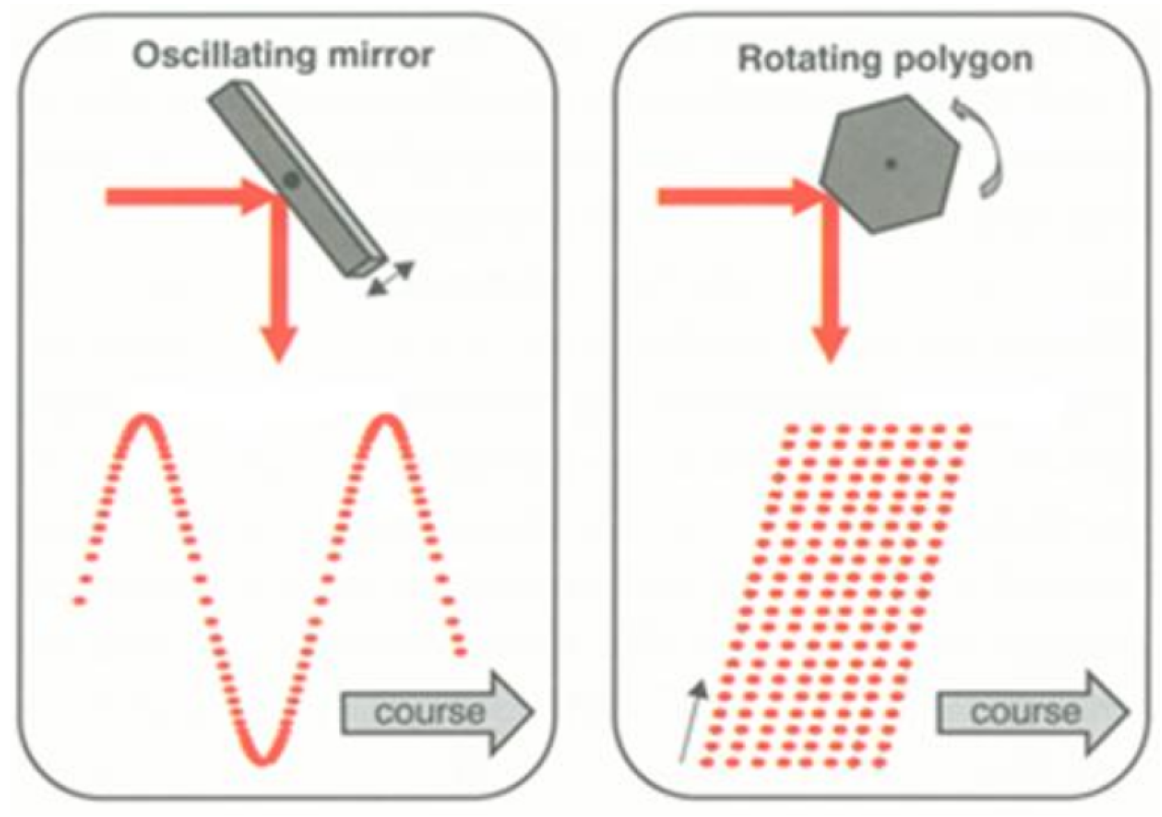
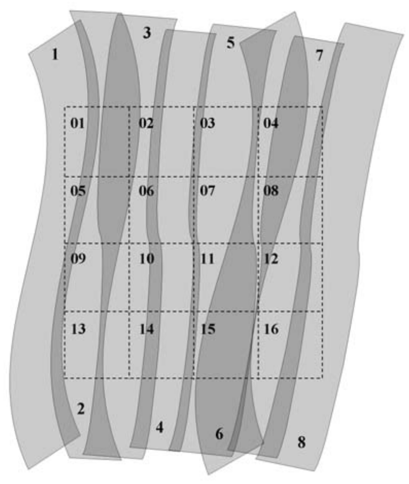
The input of this method is a set of scan lines, which can be a complete flight line or pieces of it. A scan line can be defined as the set of points recorded during the scanning mechanism rotation along the field of view. Scan lines are generally acquired in a zigzag or a parallel pattern, depending on the scanning mechanism (see Figure 1). Consecutive scan lines during the same flight course form a flight line, which is stored in an LAS file [19] (see Figure 2). The stored LiDAR points follow the format established in the LAS specification, which defines the number, order, and data type of the data fields.
The LiDAR data must meet two requirements. First, points must be georeferenced. Georeferencing is the process of transforming scanner’s coordinates into a real-world spatial system. LiDAR scanners record data in its own coordinate system, which must be integrated with GPS (Global Positioning System) and IMU (Inertial Measurement Unit) data. Furthermore, these sensors typically use different sampling rates, so data must be interpolated. While this is generally granted for offline data, in the case of real-time processing, a scanner with this capability is needed. Second, individual scan lines must be identifiable. In the case of LAS data, this information is provided in the scan direction field and edge of flight line field. In fact, just one of these two fields is enough to identify scan lines. For simplicity in the processing, the points within each scan line must follow the same scanning direction. This is the case when data have been acquired with a rotating polygon mechanism. If an oscillating mirror mechanism is used instead, it is needed to invert the point ordering in the odd scan lines, as they are recorded in both directions of the scan.
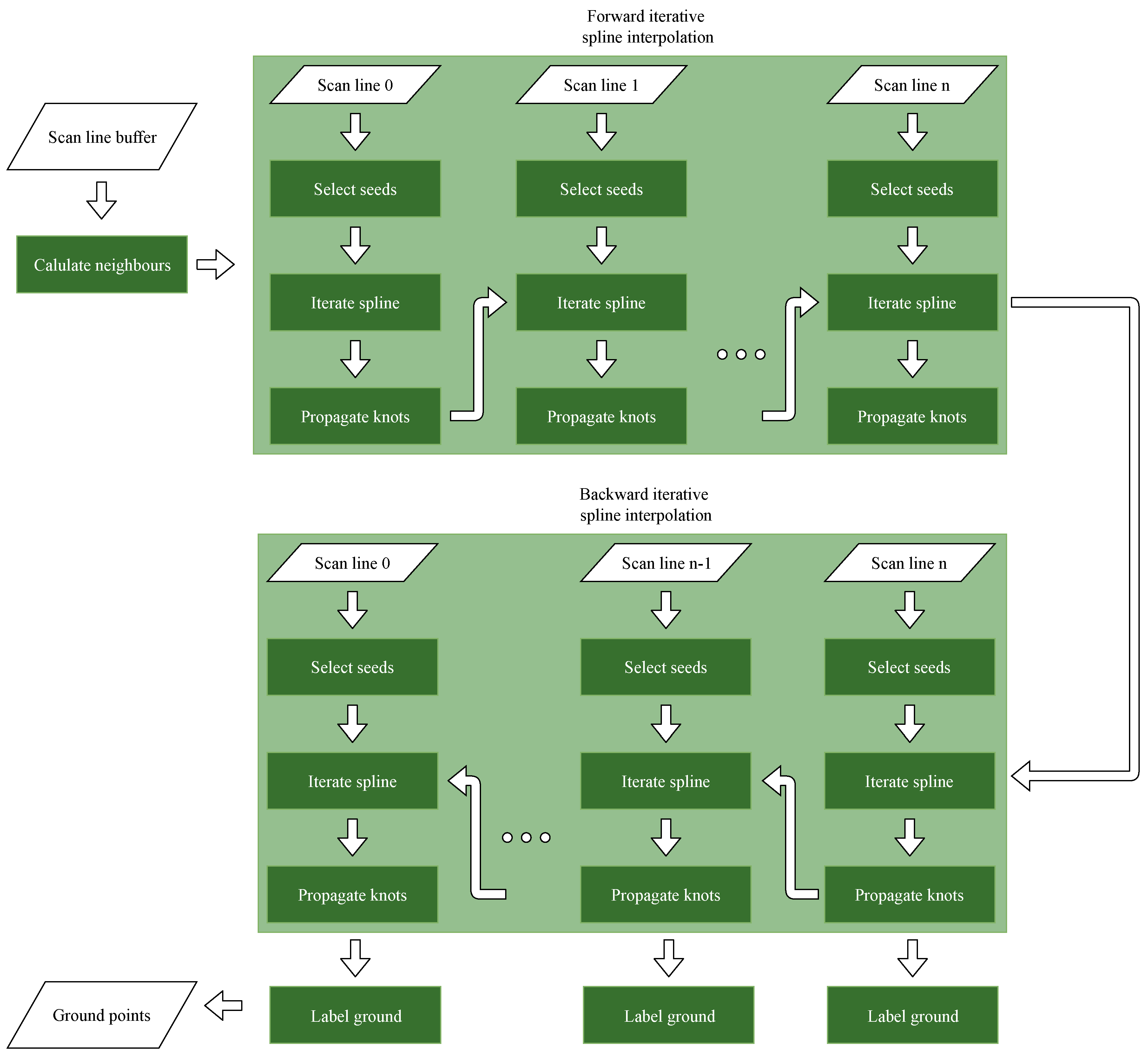
A flowchart of the whole method is depicted in Figure 3. Note that only last-return points are taken into account, as possible previous returns are assumed to be non-ground points. The first step is to calculate the set of neighbours of each point. Then, an iterative spline interpolation is performed in each scan line sequentially. First, this is done from the first to the last scan line (forward), and then, it is done from the last to the first scan line (backwards). This iterative spline interpolation consists in three main stages: (1) the selection of the initial spline knots (seeds), (2) the iterative spline interpolation, and (3) the propagation of the final spline knots to the next scan line. Once the backward iterative spline interpolation of a scan line has been performed, the resultant spline is used to identify the ground points based on their residuals. Following, we describe each one of these steps.

2.1. Neighbour Calculation

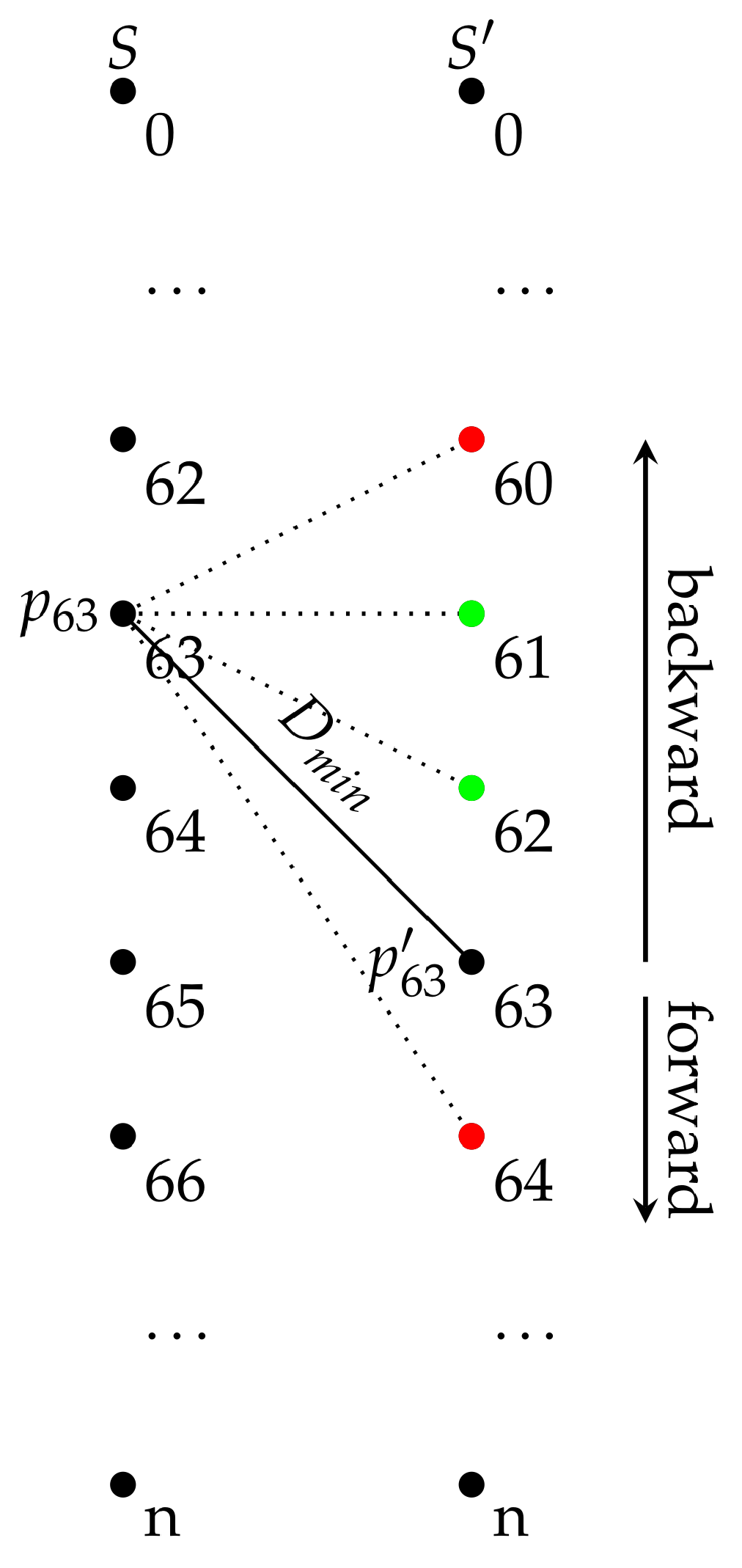
For each point, the closest point in the previous scan line and the closest point in the next scan line are calculated in this initial step. We further refer to these neighbours as the perpendicular neighbours. A perpendicular neighbour of a point can be calculated by brute force, computing all the distances from the point to all the points in the adjacent scan line and keeping the closest. Nevertheless, this is inefficient and severely increases the computing time. Moreover, it is reasonable to expect that a perpendicular neighbour will have a similar index within the scan line. This assumption can be exploited to speed up the neighbour search. The idea is to start the search at the adjacent point with the same index and to continue the search backwards and forward while the distance is being reduced. The process is depicted in Figure 4. This calculation is faster the more similar the point spacing is in both scan lines, as it leads a point and its neighbour to yield a similar index. Therefore, its speed is influenced by the acquisition procedure to some extent (see Section 4.1).

2.2. Seeds Selection

Before performing the interpolation, a set of initial knots, known as seeds, are selected. The number of seeds depends on the interpolation algorithm. The Akima interpolation algorithm [22] is used in this work, which requires a minimum number of 5 seeds. For its selection, the scan line is split into 5 segments of equal length and the lowest point in each segment is elected as a seed point. Seed points are assumed to be ground points. This assumption is acceptable when the length of the scan line is reasonably large. More specifically, this assumption is guaranteed when the length of each segment is larger than the largest non-ground object of the scene. Therefore, the length of the generated scan line must be taken into consideration when tuning the parameters of the LiDAR survey. The optimal scan line length can be calculated as follows:
S W = α n L , α [ 0.5 , 1 ]
where α is an user-defined constant (ideally 1), n is the number of scan line segments (5 in our case), and L is the largest non-ground object size. More details on this aspect are given in Section 5.1.

2.3. Iterative Spline

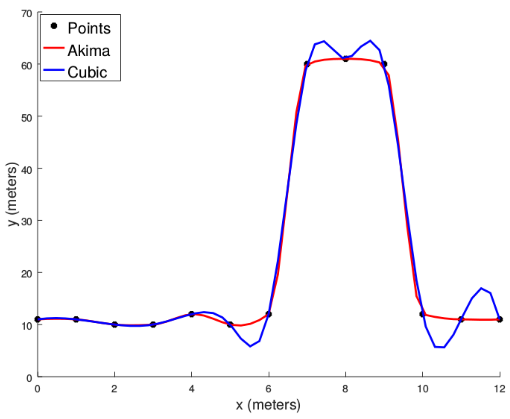
Based on the seeds, an initial interpolation of the scan line is performed. The Akima algorithm is a continuously differentiable sub-spline interpolation built from piecewise third-order polynomials. An important feature of this method is its locality: Function values on the interval [ x i , x i + 1 ] depend only on its neighbourhood f i 2 , f i 1 , f i , f i + 1 , f i + 2 , f i + 3 . The advantage of this fact is twofold: First, this method does not lead to unnatural wiggles in the resulting curve (see Figure 5), and second, it is computationally efficient as there is no need to solve large systems of equations.
The LiDAR 3-D points are projected into 1-D as follows: Its original coordinates { x , y , z } are converted into { x , y } , where x is the 2-D euclidean distance to the first point of the scan line and y = z . Note that x values must be monotonically increasing, so duplicated values are removed.
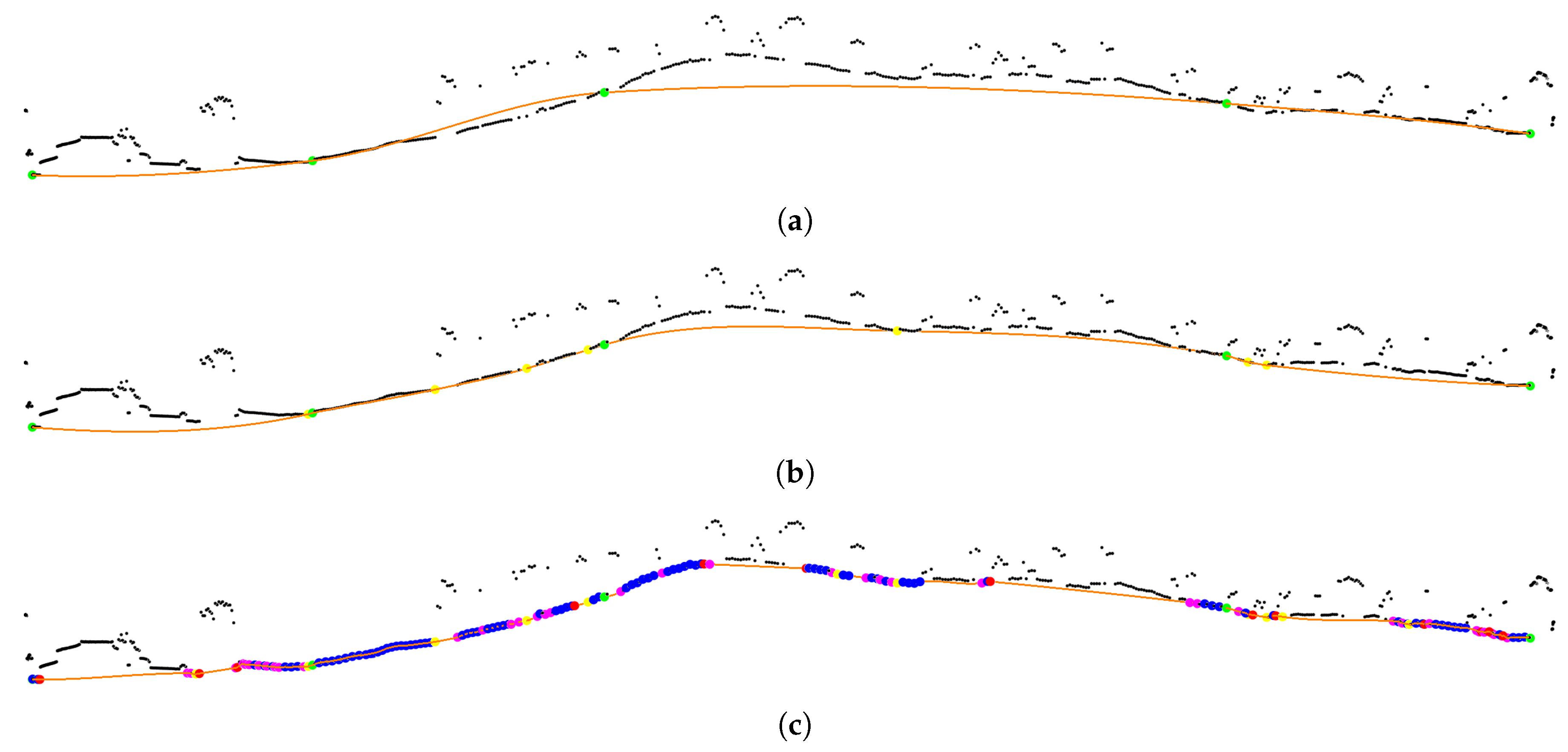
The proposed iterative interpolation consists in the execution of three stages: (1) interpolation, (2) push down, and (3) push up. The spline passes through a set of knots K = { ( x i , y i ) : 0 , 1 n } . The idea is to iteratively refine the spline by adding new knots into K. The steps are as follows:
  • The interpolation of the spline is performed. In the first iteration, K consists of just the seed points, and the initial spline is a rough estimation of the ground level (see Figure 6a).
  • In the push down stage, the spline descends into the ground level by adding ground points under the spline into K (see Figure 6b). For each knot pair ( k i , k i + 1 ) , the point with the largest residual under the spline is added into K if this residual is higher than a tolerance threshold T, so that only significant residuals are considered. An adequate value for this threshold is between one and two times the vertical accuracy of the LiDAR data. In this work, T = 0.15 m is used. After processing all knot pairs, if K has new points, we return to step 1; otherwise, this stage ends.
  • In the push up stage, the spline raises by adding ground points above the spline into K (see 
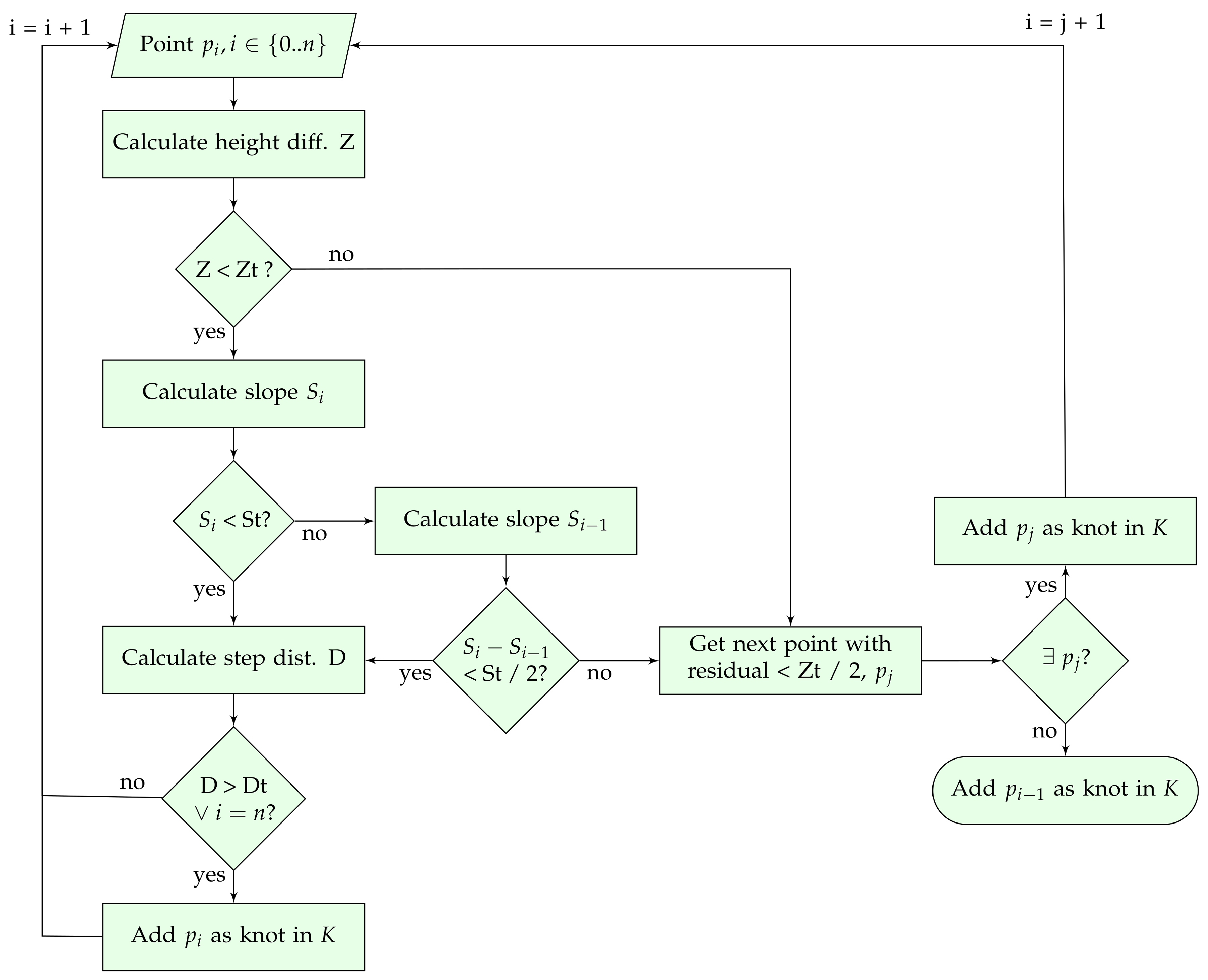
Figure 6c). The idea is to start at a known ground point and to consider the next point as ground as long as the transition is smooth. This is accomplished by a 1-D bidirectional labelling algorithm. For each knot, both forward and backward labelling are conducted. The labelling process is shown in Figure 7. The process starts at the next point of the knot. This point has to fulfil three constraints based on height difference, slope, and step distance. The calculation of these constraints are given by Equations (2)–(4). First, the pairwise height difference must be lower than a given threshold Z t . Second, the pairwise slope must be lower than a given threshold S t or the slope change (if available) must be lower than the half of S t . Third, the 2-D distance to the previous knot must be higher than a given threshold D t . This last constraint limits the number of points that will be labelled as knots, so that only meaningful knots are added, as processing all knots will increase the computational demand of the interpolation with little contribution to its accuracy. The height and slope thresholds can be tuned for a particular data to obtain better results. Common values can be widely found in the literature. Our suggestion is to use as default parameters Z t = 0.5 m and S t = 45 or S t = 60 for urban or rural sites, respectively. For the step distance threshold, we have found experimentally that D t = 1 m provides the best trade-off between accuracy and throughput. If the point does not fulfill the height or slope constraints, the next point yielding a low residual is added into K and the labelling continues in that point. The process ends if a knot is reached. Finally, if K has new points, we return to step 1; otherwise, the iterative spline interpolation finishes.
    Z i = z i z i 1
    S i = arctan z i z i 1 ( x i x i 1 ) 2 + ( y i y i 1 ) 2 , S i π 2 , π 2
    D i = ( x k x i ) 2 + ( y k y i ) 2 , with k as the index of the previous knot

2.4. Knot Propagation

The knot propagation is performed after the iterative spline interpolation. Its goal is to avoid errors when ground filtering is executed on each scan line individually without knowledge of the previous filtering. For example, in high-slope terrains, few ground points might not be identifiable for a given scan line, resulting in an inaccurate spline and causing several points to be mislabelled. However, this can be mitigated if the spline of the previously filtered scan line is considered.
The process is as follows: Let K be the set of knots of a scan line S after the iterative spline interpolation and K be the set of knots of the next scan line S to be processed, which is initially empty. The goal is to propagate the knots of K into K . Propagating a knot means that its perpendicular neighbour will be added into K . In order to be propagated, a knot has to fulfill the same but more restrictive height, slope, and step distance constraints than in the push up stage described previously. In particular, the height and slope thresholds used are reduced to half. Also, if a knot fulfils the height and slope constraints but the step distance is lower than D t , the knot is ignored. However, if a knot does not fulfill the constraints but the step distance is higher than D t , the last ignored knot is propagated. This way, the gap between propagated knots is reduced in the case of non-fulfilling knots.
Therefore, at the first iteration of the iterative spline interpolation, the initial knots of a scan line are formed by the selected seed points plus the knots propagated from the previous scan line.

2.5. Ground Labelling

Finally, the ground points of each scan line are identified using the resulting spline after forward and backward interpolation. For each point, the residual to the spline is calculated, and if this residual is lower than the tolerance threshold T, the point is labelled as a ground point.

3. Results

3.1. Quantitative Evaluation

The benchmark dataset provided by the International Society for Photogrammetry and Remote Sensing (ISPRS) Working Group III/3 [24] is the standard dataset used to evaluate and compare ground-filtering algorithms. This includes fifteen study sites with unique terrain conditions that are considered challenging to filter. Nevertheless, this dataset is not used in this study for two reasons. First, the provided LAZ files [25] do not provide information to identify the scan lines. In fact, the two related fields, scan direction and end of flight line, are set to zero. Second, even with such information available, the scan lines are particularly narrow and their length is not suitable for our method. In our approach, scan lines are initially split into 5 segments to determine the seeds for the initial spline interpolation (see Section 2.2). The length of the scan lines in the ISPRS dataset is about 150 m, so that each segment would have approximately 30 m of length, and larger objects clearly exists in these scenes. This will cause some of the seeds to be placed on top of non-ground objects, resulting in critical errors. Because of this, we instead generate a synthetic ground truth to evaluate the method quantitatively.
Synthetic ground truth was generated using the Heidelberg LiDAR Operations Simulator (HELIOS) [26]. Both urban and rural scenes were built. The urban scene was created based on OpenStreetMap (OSM) data [27]. The city of Heidelberg was chosen because of its rich OSM information. The 2-D OSM data was converted into a 3-D mesh using OSM2World [28]. The rural scene was generated by using a predefined terrain model and by randomly placing models of trees and buildings. The model’s wavefront OBJ (Wavefront 3D Object File) and MTL (Material Template Library) files were modified so that the polygons corresponding to ground surfaces are identified by HELIOS. This way, when running the simulation, pulse returns from these polygons are automatically labelled as ground points, hence generating the ground truth. The urban survey consists in an airborne laser scanning one flight strip of 1 km at a flying height of 700 m and speed of 30 m/s. A Leica ALS50-II sensor was configured with a scan angle (FOV, Field of View) of 50.5 (see Section 5.1 for justification), a scanning frequency of 60 Hz, and a pulse rate frequency of 100 KHz. The rural survey consists in an UAV-borne laser scanning one strip of 600 m at a flying height of 300 m and speed of 20 m/s. A Rielg VUX-1UAV sensor was configured with a scan angle (FOV) of 45 , a scanning frequency of 100 Hz, and a pulse rate frequency of 100 KHz.
The default parameters proposed in Section 2.3 were used. Results are depicted in Figure 8, and the kappa coefficients and error rates are shown in Table 1. In the urban scene, the main error source is commission error (Type II error) present in the railway and in the base of some building facades (see Figure 8c). In the rural area, the main error source is omission error (Type I error) present in hilly terrains at the boundaries of the scene (see Figure 8e). Given its high slope, it is quite challenging to label hilly areas as ground. Also, commission error is present in some lower roofs that reach the ground (see Figure 8d). Overall, these results show the suitability of our method.

3.2. Qualitative Evaluation

Visual inspection was carried out using real LiDAR data, particularly, private data from Alcoy and Trabada, both in Spain, and public data from Vaihingen, in Germany. Information about these data is shown in Table 2. Alcoy is a rural site with areas with high slope, abrupt height changes in the terrain, and some cliffs. Trabada is a rural area mixing well-defined lands with areas of dense vegetation. Vaihingen is an urban site with the characteristics of a typical European city. One flight line was processed for each site. For simplicity, only three representative areas are shown for each site. The default parameters proposed in Section 2.3 were used. Results are shown in Figure 9, Figure 10 and Figure 11 and the highlighted errors are in Figure 12. Apart from the labelled ground points, their triangulated irregular network (TIN) computed with FugroViewer [29] is also shown to aid the evaluation.
In Alcoy, there are no significant errors when processing slope terrains (see Figure 9a), flat areas with small but abrupt height changes (see Figure 9b), or irregular terrains (Figure 9c). Although, when dealing with irregular terrain, some ground points near the edges of the cliffs are sometimes missing, producing a less-detailed surface (see Figure 12a). In Trabada, few points located in the lower parts of trees are mislabelled as ground, giving the ground surface a rough look. This effect is related to the slope threshold; by increasing this threshold from 45 to 60 in rural areas, the labelling of sloped terrain improves but also increases the overall roughness of the extracted surface. In Vaihingen, there are no appreciable errors, in part, because most of the terrain is fairly flat. Finally, we have observed that the filtering sometimes struggles in some areas near the edges of the scan lines, particularly when dealing with high sloped terrain or vegetation (see Figure 12c,d). In such areas, no ground points are labelled, leading to a less-detailed surface (see Figure 12b). This happens because the interpolation is not being performed at the boundaries of the scan line. More specifically, there is a set of points between the first point of the scan line and the first knot of the spline that heavily relies on the seed propagation in order to identify ground points, which is not always possible in these areas with high height and slope changes. Overall, the results are satisfactory and the method can filter ground points successfully for both urban and rural sites using the default parameters.

3.3. Computational Performance

The execution times of the reference C implementation for the Alcoy, Trabada, and Vaihingen data samples are shown in Table 3. Measurements were taken on a workstation with an Intel Core i7-4790 processor, 16 GB of RAM memory, and a Linux (Ubuntu 14.04.5 LTS) operating system. In the Alcoy and Trabada data, the algorithm is able to process nearly 1 million points per second. However, in the Vaihingen data, the throughput decreases significantly to 320,000 points per second. This is because of point accumulation present in the data, which slows down the neighbour search. The topic of point accumulation is further addressed in Section 4.1.

4. Embedded System Implementation

In order to demonstrate the portability of the proposed method to embedded systems while maintaining its good performance, we implemented it in a ZedBoard platform [33]. This is a low-cost, low-power consumption development board, and it is shipped with a Zynq-7000 System-on-Chip (SoC) from Xilinx, 512 MB of DDR3 RAM, and several I/O peripherals such as a 1-Gb ethernet module and an SD card reader. The Zynq SoC integrates a 32-bit dual-core ARM Cortex-A9 CPU and a low-range Z7020 FPGA [34], which allows the implementation of simple custom hardware accelerators.
In this proof of concept, we deployed two different implementations in the Zedboard. The first implementation is just a porting of the original C source code, developed for the x86-64 architecture, to the ARM v7 architecture. The results and performance comparisons for different LiDAR data are described in Section 4.1. The second implementation is a custom hardware accelerator on the FPGA for precomputing the perpendicular neighbours. The software–hardware system developed and the results of the evaluation test performed are described in Section 4.2. Power and energy consumption is shown in Section 4.3.

4.1. CPU Implementation

Since a bare-metal implementation (non-OS support) of the method in the Zynq SoC does not provide enough flexibility for future code development and enhancements, a 32-bit embedded Linux distribution (Xilinx Linux kernel 4.14.04 and an Ubuntu 16.04 root file system) was deployed in the ARM Cortex-A9. For porting the original C code to the ARM Cortex-A9, we tried to avoid any substantial code changes. The pre-compiled GNU GSL libraries [35] with hardware floating-point support for the ARM Cortex-A9 were used, and the OpenMP [36] directives presented in the original code were preserved. We show the trace results for the Alcoy, Trabada, and Vaihingen data samples in Table 4. The timing figures are shown for the tests run in Zedboard (only in the dual-core ARM CPU run at 667 MHz).
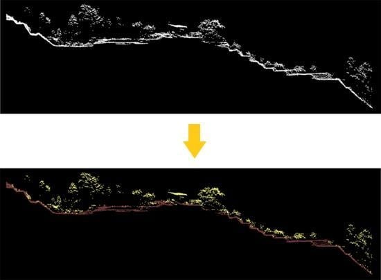
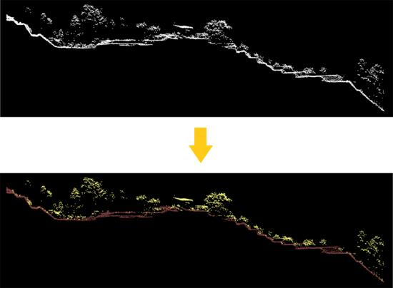
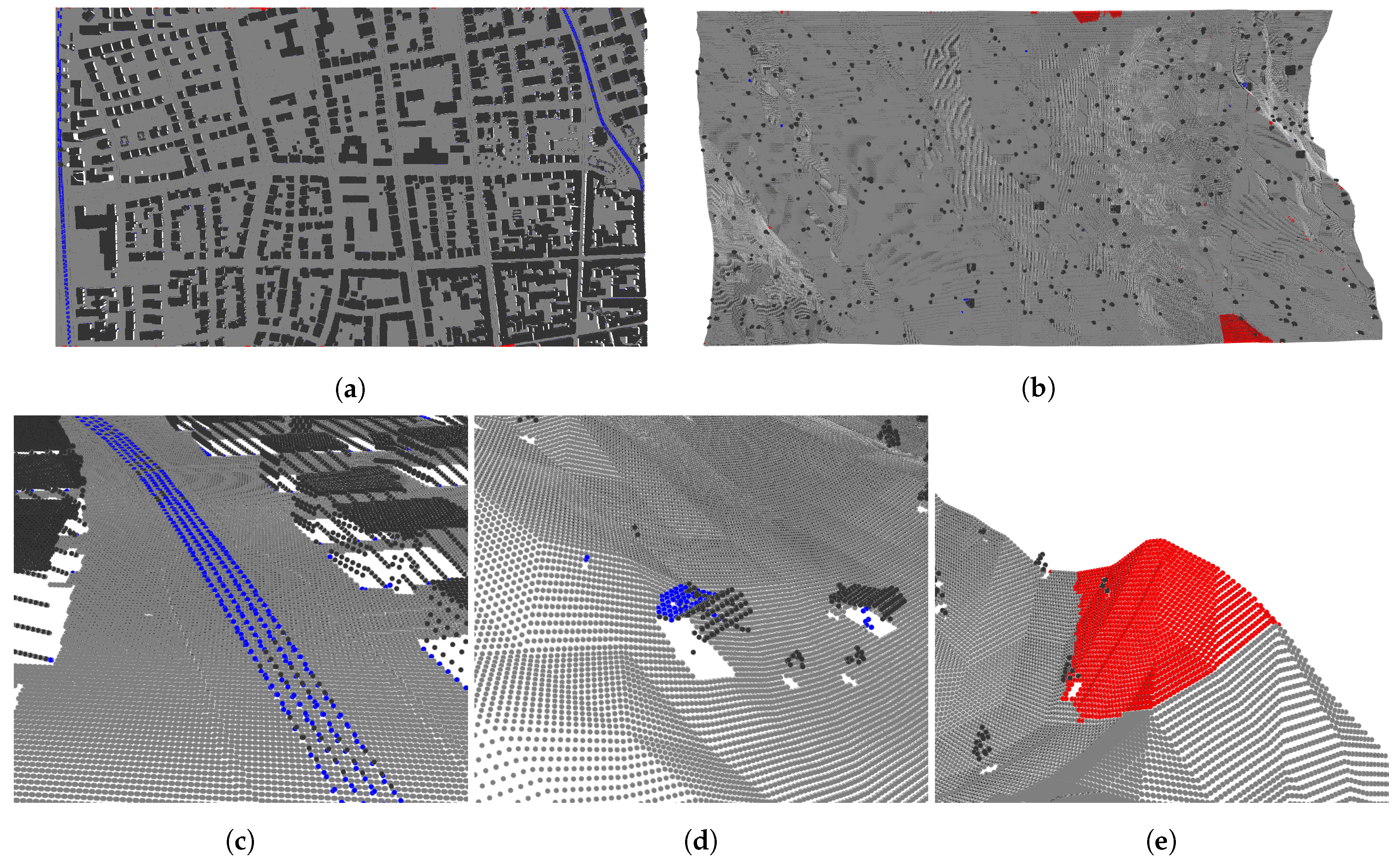
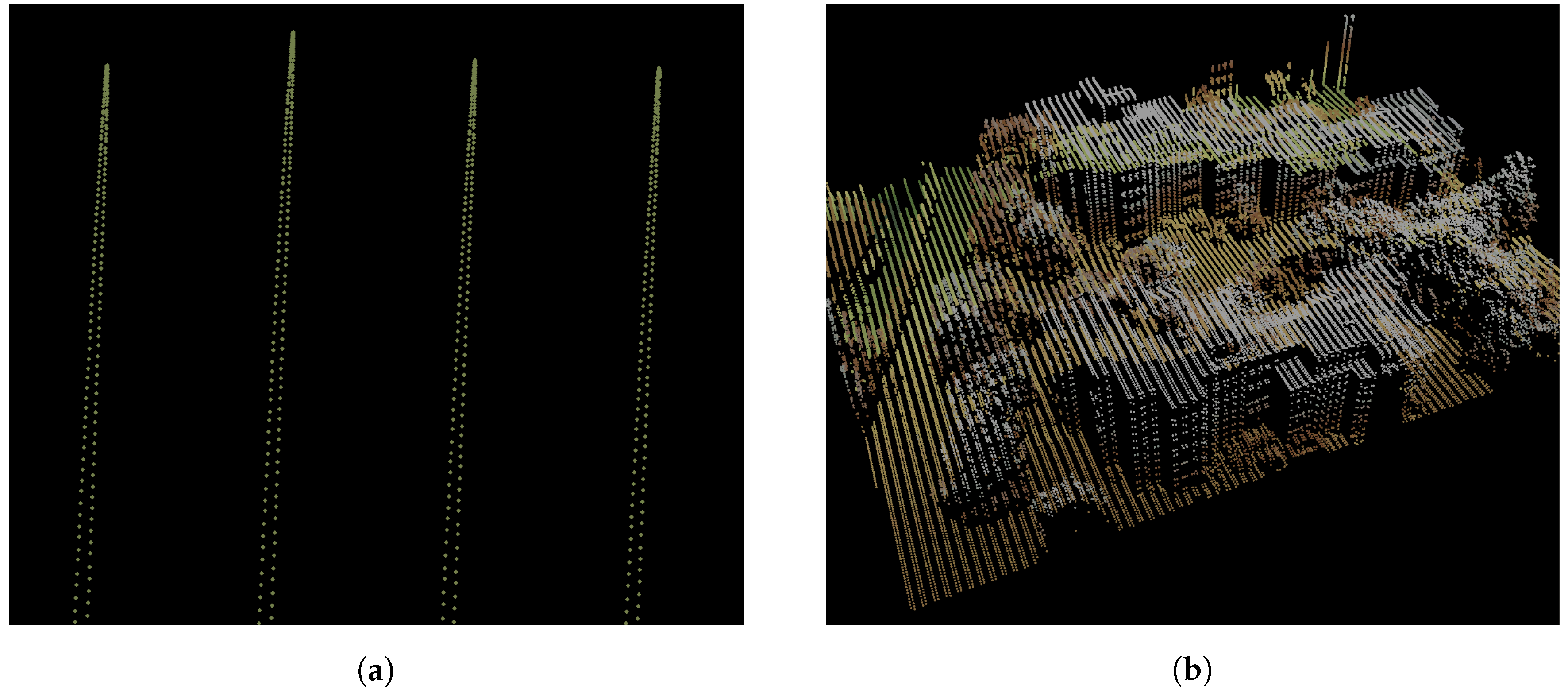
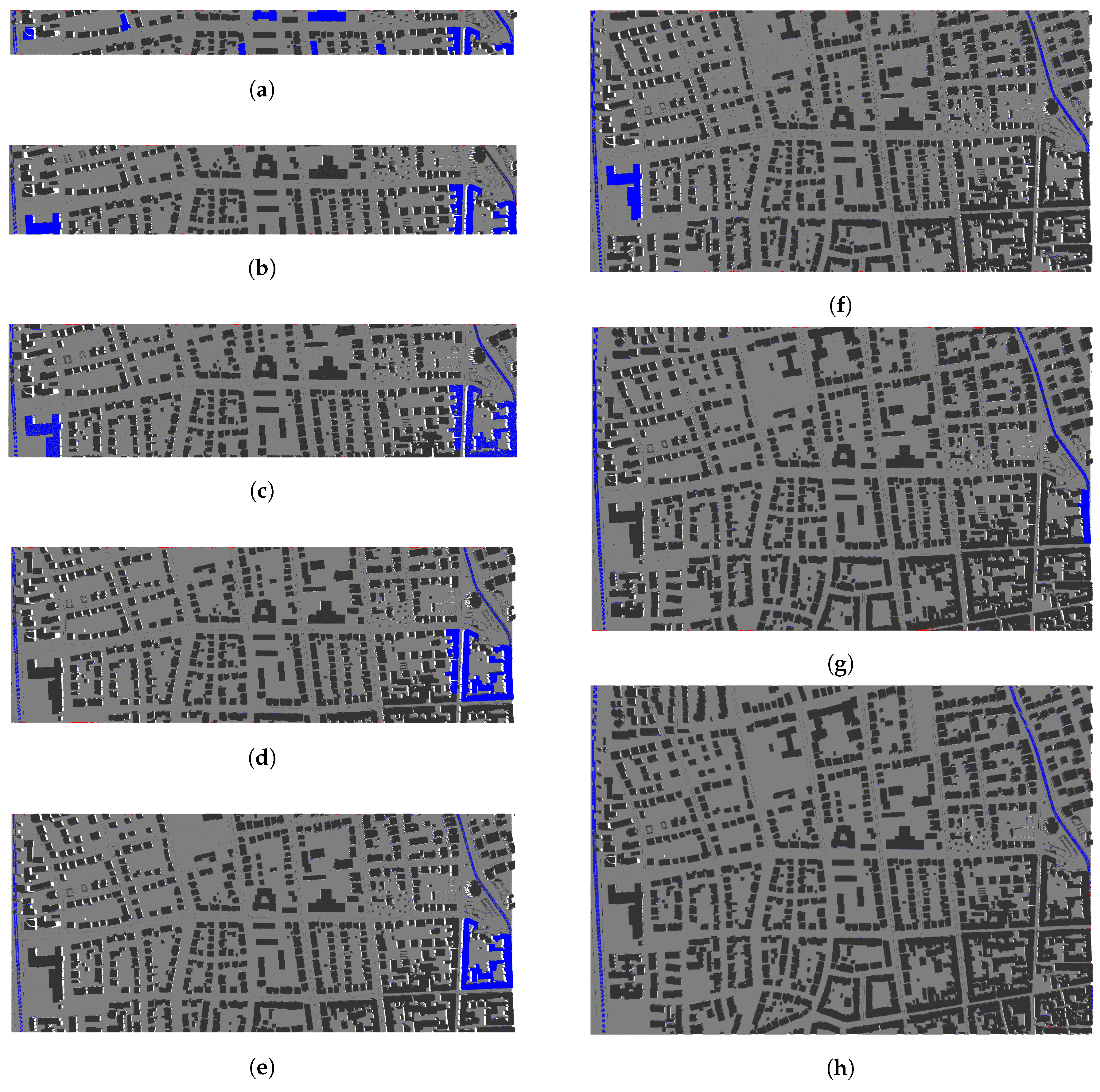
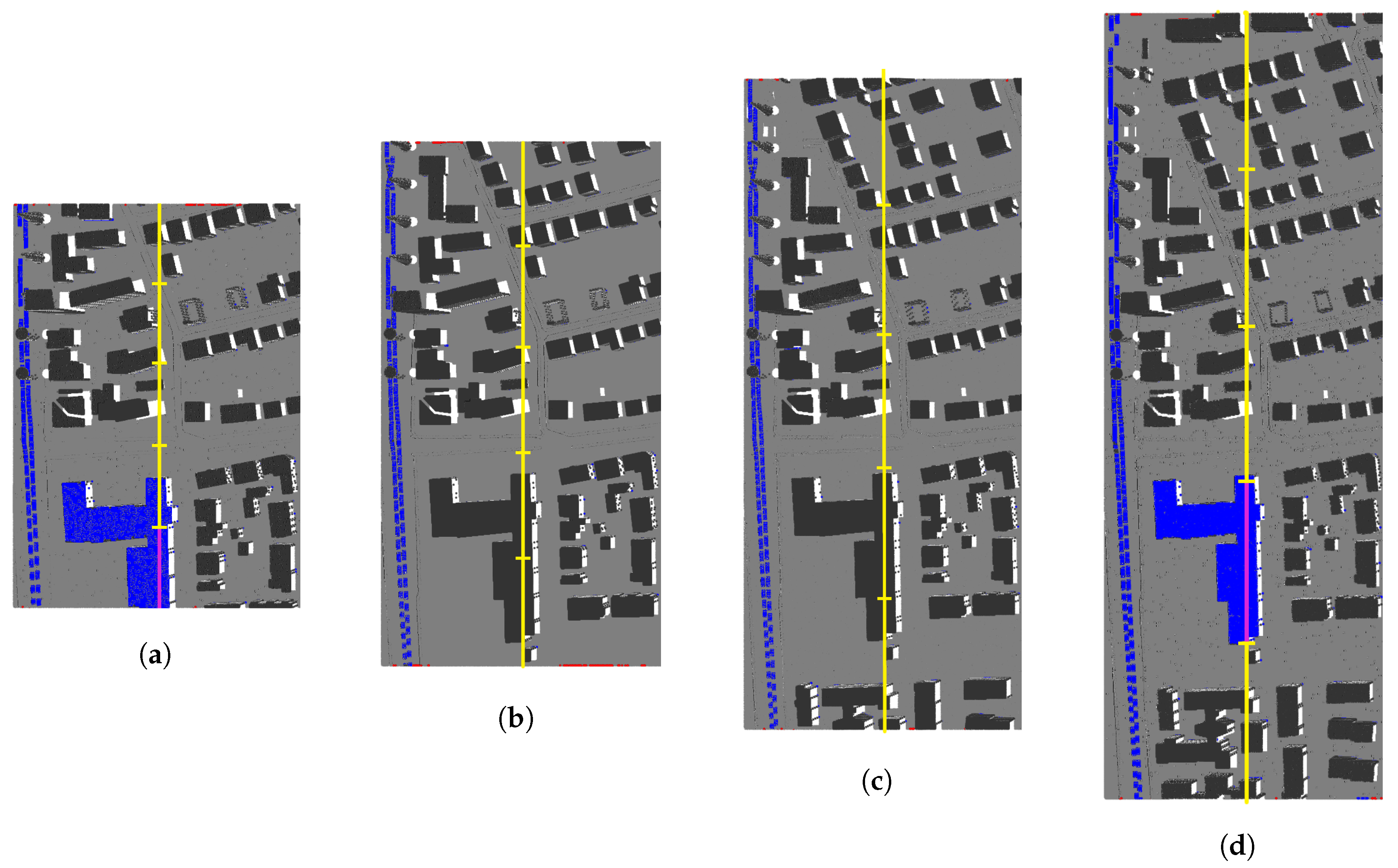
Note that the throughput in the Vaihingen sample is significantly lower than in the other samples. This is because the calculation of neighbours is quite costly in this particular sample. This is attributed to an accumulation of points at the sides of the point cloud. On the one hand, the deceleration of the sensor’s oscillating mirror when changing the scanning direction increases the number of points recorded at the edges of the point cloud (see Figure 13a). On the other hand, the higher the scan angle, the higher the coverage of building facades, which also increases the number of points recorded (see Figure 13b). These accumulations of points are detrimental for the computational performance of the neighbour search, which relies on the assumption that points of two adjacent scan lines present a similar point distribution. Furthermore, it is expected for point clouds generated in real-time to yield a more irregular scan-line point distribution than fully post-processed point clouds. In order to increase the throughput of the algorithm in such situations, a hardware accelerator was implemented on the PL (Programmable Logic) of the Zynq SoC.

4.2. Programmable Logic Acceleration

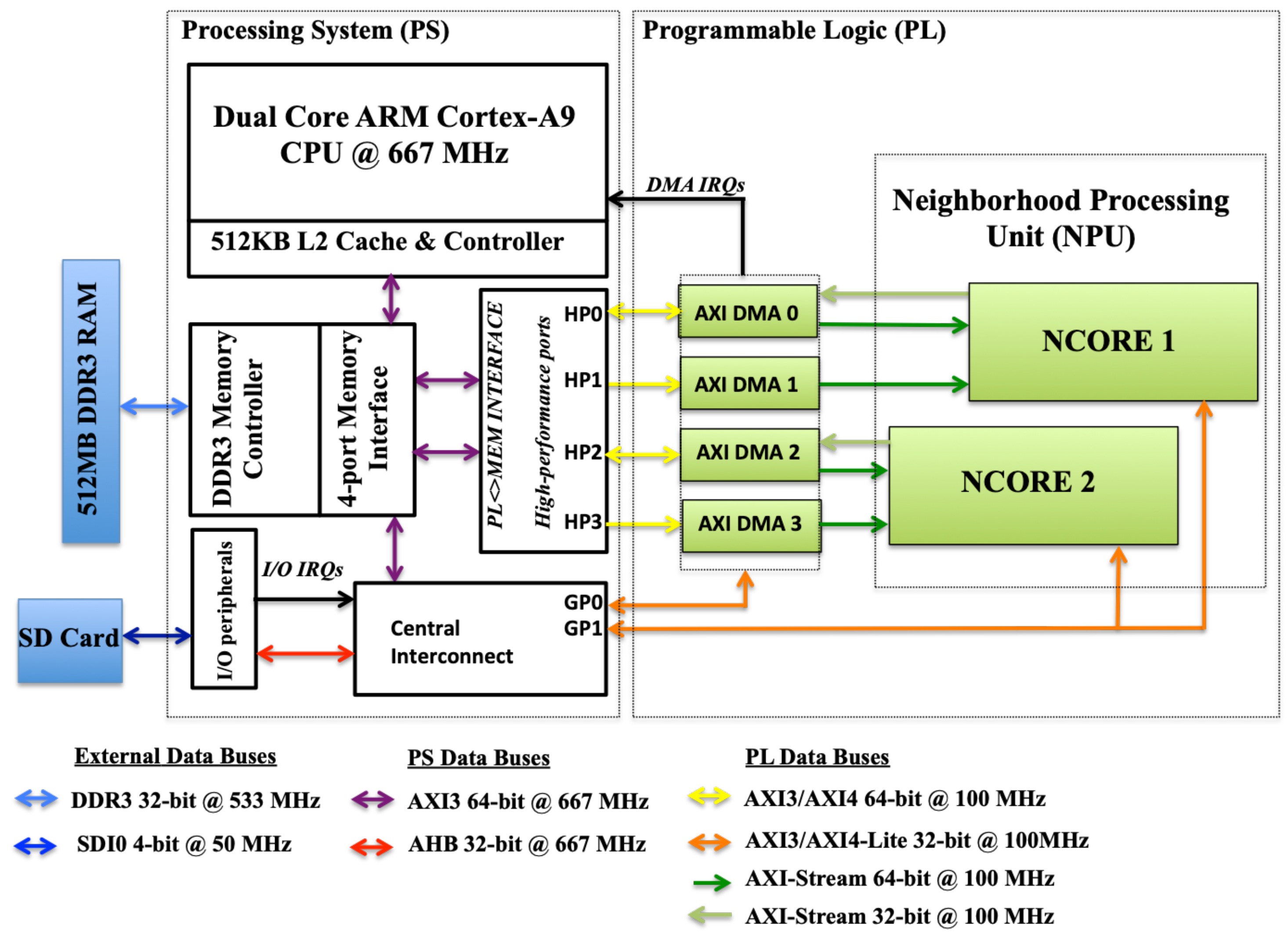
The hardware architecture of the system implemented is shown in Figure 14. The hardware accelerator consists of two Neighbourhood Search Cores (NCOREs), each one computing the neighbours of different scan lines in parallel. Each NCORE communicates with the on-board DDR3 RAM and the CPU via DMA (Direct Memory Access) and high-performance (HP) ports. For optimal memory bandwidth use, two 64-bit DMA Controllers (AXI-DMA in Figure 14) are needed for each NCORE implemented and run at the same clock speed as the NCORE. This bandwidth constraint is only required for reading data from RAM, since write operations to RAM are less frequent. Both the internal frequency of the PL and the input frequency run at 100 MHz, which is the maximum that allows processing one datum per cycle with the current design. The ARM cores in the PS (Processing System) of the Zynq SoC run at 667 MHz.
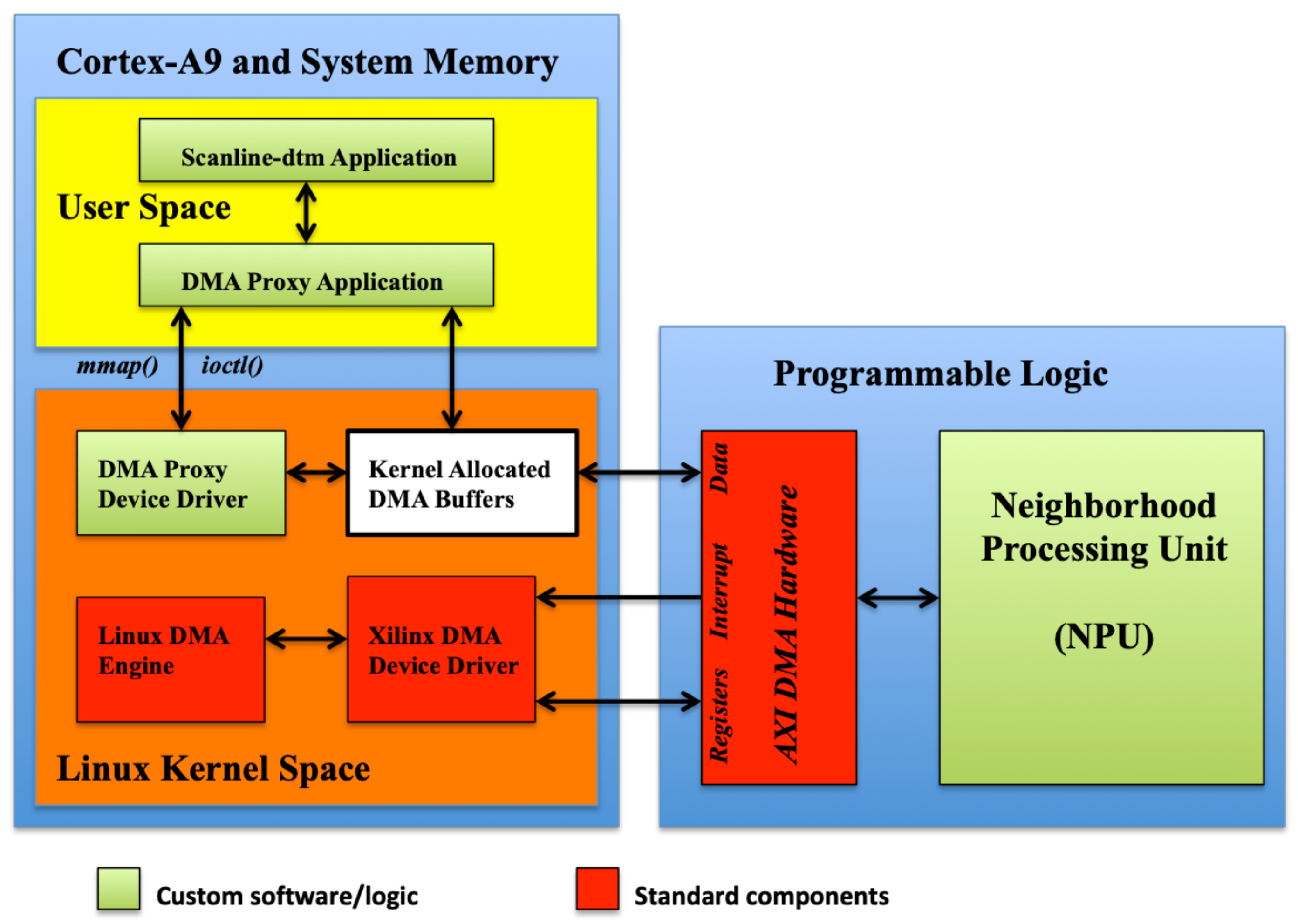
To interact with the hardware acceleration from the software application, which runs in the Linux environment in the ARM CPU, we rely on the DMA Engine framework and Xilinx DMA device drivers. A general view of the architecture of the software-hardware system deployed is shown in Figure 15. In addition to the acceleration hardware, we developed a Linux kernel character driver and a DMA proxy user application. These software codes provide the control logic for the communication of the DMA controllers built in the FPGA with the CPU via RAM.
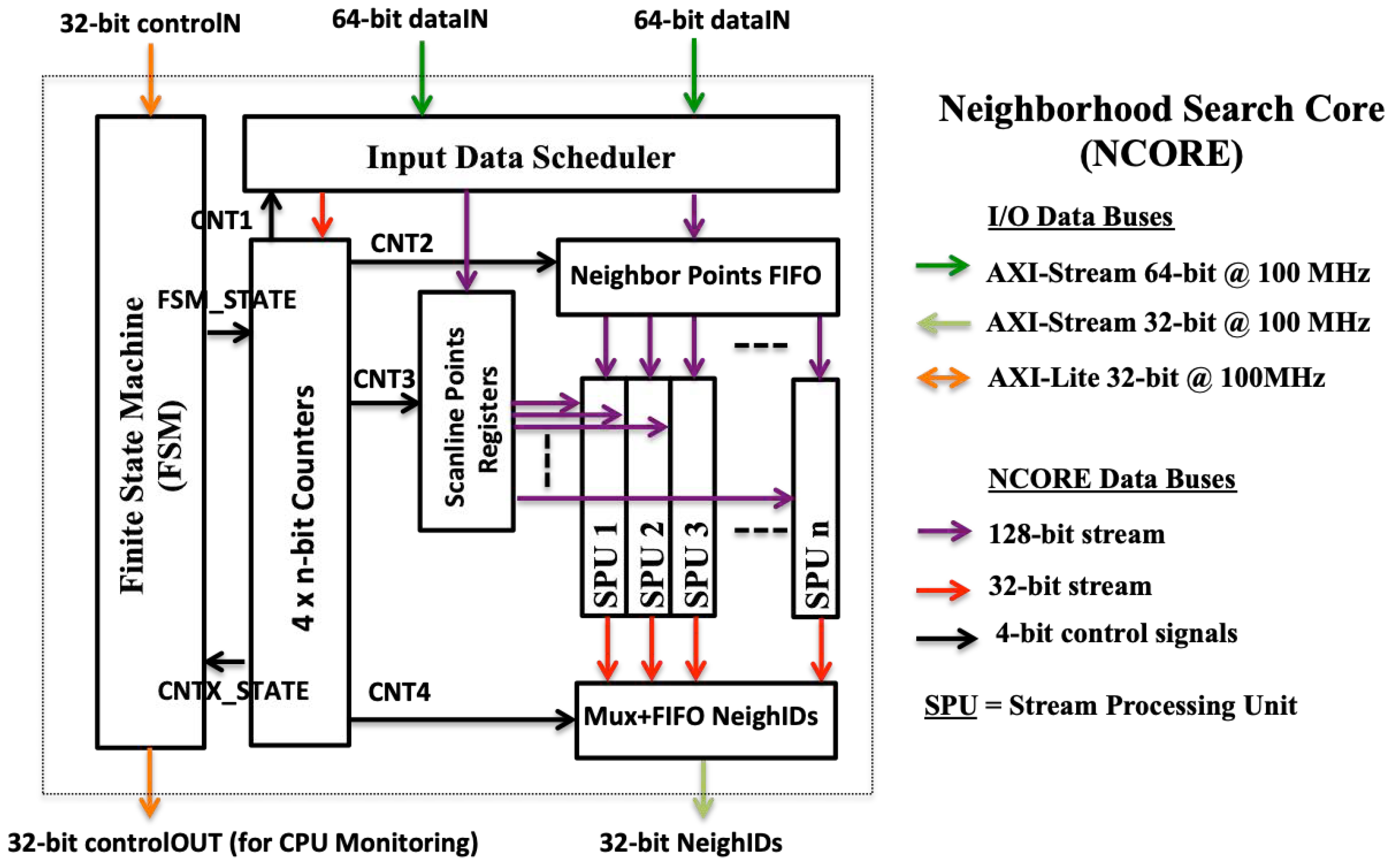
Finally, the architecture of the NCORE is shown in 
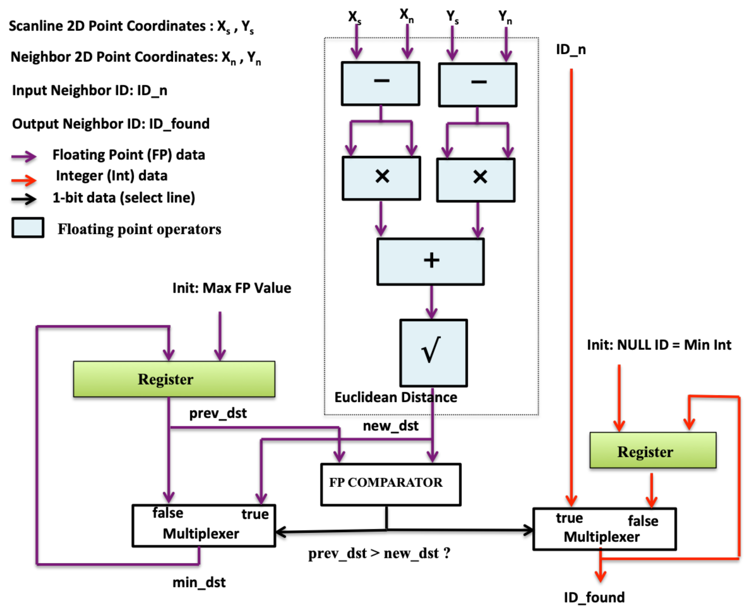
Figure 16. In addition to the parallelism at the scan-line level (one scan line search per NCORE), each NCORE can search concurrently for the neighbours of several consecutive points of the same scan line, issuing one search for each SPU (Stream Processing Unit) implemented in the NCORE. The structure of the SPUs is shown is Figure 17. Therefore, the total parallelism implemented in the hardware accelerator is given by the number of NCOREs multiplied by the number of SPUs of each NCORE. The optimal number of NCOREs is given by the ratio of the available DDR memory bandwidth with respect to the NCORE throughput (The NCORE throughput is proportional to the clock frequency and inverse to the maximum cycle interval between two consecutive data inputs.). For our Zynq FPGA this factor is close to two. On the other hand, we have implemented one core with 2 SPUs (NCORE 1) and the other (NCORE 2) with 3 SPUs. Therefore, the total number of SPUs (and the parallelisation factor) is 5.
The resources of the FPGA used and the total use percentage are summarised in Table 5. The FF (Flip-Flop) resources are used for implementing registers and fast data storage. LUT (LookUp Table) are used for implementing combinational logic while the DSP48E are building blocks used in arithmetic (fixed and floating-point) operations. The performance is limited mainly by the available LUT resources, since embedding additional SPUs in a CORE does not modify the memory bandwidth usage.
To provide an estimation of the achievable acceleration of the execution time of the neighbour search of the scan-line points, we run the Vaihingen sample in the Zedboard with and without using the PL hardware acceleration. The results of these tests are shown in Table 6. We show that the execution time of the neighbours search can be accelerated by a factor of 3.5 with a (non-optimised) custom hardware accelerator.

4.3. Power and Energy Consumption

Two different methods have been used in order to estimate power consumption. For early estimation of the Xilinx Zynq SoC power consumption during the cycle design, we have used the Xilinx Power Estimator (XPE). The XPE is a spreadsheet-based tool that provides detailed power and thermal information based on design information such as resource use and clock frequencies. For power consumption estimation of the Zedboard during execution, we use voltage measurements of the shunt-resistor mounted on the power supply of the ZedBoard. The shunt-resistor is a 10-m Ω resistor in series with the input supply line to the board; this resistor can be used to measure the current draw of the whole board. The current draw can be used to calculate the power consumption of the board using Ohm’s law and the supply voltage. As the power supply voltage is 12 V, the power consumption of the board can be obtained by measuring the voltage over the current sense resistor and by inserting the measured value into Equation (5).
P = V measured 10 m Ω 12 V
The power dissipation of the Zedboard during the tests performed with and without hardware acceleration was below 3 W. The results of these tests are summarised in Table 7. Energy efficiency is increased by using hardware acceleration.

5. Discussion

5.1. Survey Requirements: Scan-Line Length

As mentioned previously, the scan lines need to have a minimum length, so that the seed points for the initial interpolation are correctly selected. In order to analyse the impact of the scan-line length in our method, we generated synthetic ground truth for Heidelberg urban site with different survey configurations to achieve different scan-line lengths. The scan-line length, formally known as swath width S W , is derived from the flying height h and the scan angle (FOV) θ , as in Equation (6) [37]. To consider different S W values, we opt to fix the flying height and to use different scan angles. The scan angle or flying height can be calculated using Equation (7).
S W = 2 h tan θ 2
θ = 2 arctan S W 2 h , h = S W 2 tan ( θ 2 )
The results are shown in Figure 18, and kappa values and total error rates are shown in Figure 19, respectively. The kappa values and total error rates improve the higher the scan-line length. With a scan line of 100 m, the accuracy metrics decrease significantly. Larger lengths achieve kappa values higher than 90%. The total error is under 5% when using a length as from 400 m. The main source of error is commission error present in large buildings. Nevertheless, there is visible commission error until use of a length of 700 m. Also, note that some errors can appear again when using larger lengths. To understand this behaviour, we now explain the influence of the scan-line segment distribution.
Consider the case of the building placed in the left side of Figure 18, which has been wrongly classified using a scan-line length of 300 m, correctly classified using lengths of 400 m and 500 m, and wrongly classified again using 600 m. This is caused because, in the four cases, the building size is larger than the scan-line segment size, which can produce misclassifications depending on the distribution of the scan-line segments. The distribution is different for each scan-line length (see Figure 20). If a non-ground object is larger than a segment but smaller than two, there is a probability for the object to be split between two segments without fully covering any segment, thus selecting valid seed points in both segments (as in Figure 20b,c). However, if the non-ground object covers a full segment, then the selected seed point will be a non-ground point instead of a ground point, which will incorrectly shift the spline upwards, causing the misclassification of the object (see Figure 20a,d). The parameter α of Equation (1) is used to set this probability. Also, it is important to mention that the survey was done so that most non-ground are aligned with the scan-line direction, which is the worst case situation.
Let us analyse an appropriate scan-line length for this site using Equation (1). The largest non-ground object is a building with an approximate largest size of 165 m. The ideal length is calculated by setting α = 1 , which results in 815 m. This would guarantee the correct selection of seeds independently from both the alignment of the objects with the scan line and the distribution of the scan-line segments. However, using such lengths may be impractical in some situations, particularly for UAV-borne laser scanning. In such cases, a smaller α can be used. Experimentally, we found that α = 0.80 offers the best trade-off between accuracy and length. In this scene, this is a length of 660 m, which derives a scan angle of 50.5 with the used survey configuration.

5.2. Comparison with other Methods

Several authors have presented new methods for ground filtering during the last years. The total error and kappa coefficients they achieved are summarised in Table 8. Note that our experiments have been conducted in a dataset different from ISPRS because, as previously explained in Section 3.1, the ISPRS benchmark is not suitable for scan-line-based processing. In fact, to the best of our knowledge, none of the scan-line-based methods have been tested with this benchmark. The proposed method yields the lowest total error rate. However, this can be partly attributed to the use of a synthetic dataset and lower accuracy values are expected when dealing with real data, as its complexity is higher. Nevertheless, tests with real data show that there is clear evidence that the proposed method yields similar accuracy values to existing methods. This is achieved without the need to train samples or to set complex thresholds and high throughput. In regard to the embedded system implementation, we are not aware of any other method tested in such platform to be compared with.

5.3. Real-Time Processing Capability

For practical application, the proof of concept implemented on the Zedboard evaluation board should be prototyped on a high-end Zynq chip. We take as a reference the Zynq Ultrascale Zcu104 [38], which has a larger bandwidth (×4 of the Zedboard), a faster CPU (a 64-bit quad-core ARM Cortex-A53 at 1.5 GHz), and more PL resources that will allow to increase the number of NCORES to four with eight SPUs per NCORE, improving the hardware acceleration. Therefore, we expect an Ultrascale implementation to have a throughput four times faster than the Zedboard implementation. The Zedboard has an average throughput in the three samples of 61,600 points per second, so we expect to reach a throughput of nearly 250,000 points per second in the Ultrascale without any modification in the source code. The user must be aware of this throughput when selecting the sensor and its configuration, as real-time processing is accomplished if this throughput is higher than the data acquisition rate of the scanner. Therefore, real-time requirements are established by the LiDAR sensor. Some examples of current laser scanners that could be used to achieve real-time processing are the Ibeo Lux HD (19,000 points/s) [39] or the Riegl miniVUX-1UAV (100,000 points/s) [40]. This is assuming a setup tuned to achieve the maximum number of measures per second, although a less demanding configuration could be used. In such a case, this implementation could cope with other scanners such as the Velodyne VLP-16 (300,000 points/s) [41]. Nevertheless, the algorithm requires the data to be georeferenced, which will certainly add some overhead in the processing. Moreover, although the power consumption estimation of the Ultrascale (9 W) is greater than the Zedboard (3 W), the energy consumption is 33% lower; therefore, the Ultrascale implementation is more energy efficient.

6. Conclusions

In this paper, an efficient method for ground filtering based on scan-line processing is presented. Its main feature is the capability to be used in real-time scenarios. The core of the processing consists of a novel 1-D iterative spline interpolation algorithm. Two-dimensional information is considered while maintaining a fast 1-D processing approach thanks to a procedure to propagate the spline’s knots. This strategy achieves a high throughput, which allows for fast ground filtering. Experiments showed that the method can perform ground filtering effectively in both urban and rural sites. Ground filtering is still challenging in areas with large non-ground objects and hilly regions. One relevant element to consider when using this method is the scan-line length, formally known as swath width, of the input point cloud. Guidelines for selecting an appropriate value when planning the survey have been provided, and its influence has been studied. Furthermore, an embedded system implementation we developed can process as many points as some current lightweight scanners can acquire with low-energy consumption. Overall, we conclude that this method accomplished real-time requirements for ground filtering.

Author Contributions

Conceptualization, J.M.S., Á.V.Á., D.L.V., F.F.R., J.C.C.D., and T.F.P.; methodology, J.M.S., Á.V.Á., D.L.V., F.F.R., J.C.C.D., and T.F.P.; software, J.M.S. and Á.V.Á.; validation, J.M.S.; formal analysis, J.M.S.; investigation, J.M.S. and Á.V.Á.; resources, D.L.V., F.F.R., J.C.C.D., and T.F.P.; data curation, J.M.S. and Á.V.Á.; writing—original draft preparation, J.M.S. and Á.V.Á.; writing—review and editing, D.L.V., F.F.R., J.C.C.D., and T.F.P.; visualization, J.M.S. and Á.V.Á.; supervision, D.L.V., F.F.R., J.C.C.D., and T.F.P.; project administration, D.L.V. and F.F.R.; funding acquisition, F.F.R.

Funding

This work was supported by the Ministry of Education, Culture, and Sport, Government of Spain (Grant Number TIN2016-76373-P), the Consellería de Cultura, Educación e Ordenación Universitaria (accreditation 2016–2019, ED431G/08, and ED431C 2018/2019), and the European Union (European Regional Development Fund—ERDF).

Acknowledgments

The authors would like to thank Juan Martín Herrera-Vidal Núñez for providing software to aid the generation of the rural synthetic data. The Vaihingen data set was provided by the German Society for Photogrammetry, Remote Sensing, and Geoinformation (DGPF) (Cramer, 2010): http://www.ifp.uni-stuttgart.de/dgpf/DKEP-Allg.html. Babcock International and LaboraTe group (USC) provided the Alcoy and Trabada data, respectively.

Conflicts of Interest

The authors declare no conflict of interest.

References

  1. Meng, X.; Currit, N.; Zhao, K. Ground Filtering Algorithms for Airborne LiDAR Data: A Review of Critical Issues. Remote Sensing 2010, 2, 833–860. [Google Scholar] [CrossRef] [Green Version]
  2. Axelsson, P. DEM generation from laser scanner data using adaptive TIN models. Int. Arch. Photogramm. Remote. Sens. 2000, 33, 110–117. [Google Scholar]
  3. Meng, X.; Wang, L.; Silván-Cárdenas, J.L.; Currit, N. A multi-directional ground filtering algorithm for airborne LIDAR. ISPRS J. Photogramm. Remote. Sens. 2009, 64, 117–124. [Google Scholar] [CrossRef] [Green Version]
  4. Chen, C.; Li, Y.; Li, W.; Dai, H. A multiresolution hierarchical classification algorithm for filtering airborne LiDAR data. ISPRS J. Photogramm. Remote. Sens. 2013, 82, 1–9. [Google Scholar] [CrossRef]
  5. Pingel, T.J.; Clarke, K.C.; McBride, W.A. An improved simple morphological filter for the terrain classification of airborne LIDAR data. ISPRS J. Photogramm. Remote. Sens. 2013, 77, 21–30. [Google Scholar] [CrossRef]
  6. Mongus, D.; Žalik, B. Parameter-free ground filtering of LiDAR data for automatic DTM generation. ISPRS J. Photogramm. Remote. Sens. 2012, 67, 1–12. [Google Scholar] [CrossRef]
  7. Hu, H.; Ding, Y.; Zhu, Q.; Wu, B.; Lin, H.; Du, Z.; Zhang, Y.; Zhang, Y. An adaptive surface filter for airborne laser scanning point clouds by means of regularization and bending energy. ISPRS J. Photogramm. Remote. Sens. 2014, 92, 98–111. [Google Scholar] [CrossRef]
  8. Zhang, W.; Qi, J.; Wan, P.; Wang, H.; Xie, D.; Wang, X.; Yan, G. An Easy-to-Use Airborne LiDAR Data Filtering Method Based on Cloth Simulation. Remote Sens. 2016, 8, 501. [Google Scholar] [CrossRef]
  9. Hui, Z.; Hu, Y.; Yevenyo, Y.Z.; Yu, X. An Improved Morphological Algorithm for Filtering Airborne LiDAR Point Cloud Based on Multi-Level Kriging Interpolation. Remote Sens. 2016, 8, 35. [Google Scholar] [CrossRef]
  10. Chen, C.; Li, Y.; Zhao, N.; Guo, J.; Liu, G. A fast and robust interpolation filter for airborne lidar point clouds. PLoS ONE 2017, 12, e0176954. [Google Scholar] [CrossRef]
  11. Ma, W.; Li, Q. An Improved Ball Pivot Algorithm-Based Ground Filtering Mechanism for LiDAR Data. Remote Sens. 2019, 11, 1179. [Google Scholar] [CrossRef]
  12. Shan, J.; Aparajithan, S. Urban DEM generation from raw LiDAR data. Photogramm. Eng. Remote Sens. 2005, 71, 217–226. [Google Scholar] [CrossRef]
  13. Hebel, M.; Stilla, U. Pre-classification of points and segmentation of urban objects by scan line analysis of airborne LIDAR data. Int. Arch. Photogramm. Remote. Sens. Spat. Inf. Sci. 2008, 2008 38, 187–192. [Google Scholar]
  14. Hu, X.; Li, X.; Zhang, Y. Fast Filtering of LiDAR Point Cloud in Urban Areas Based on Scan Line Segmentation and GPU Acceleration. IEEE Geosci. Remote Sens. Lett. 2013, 10, 308–312. [Google Scholar] [CrossRef]
  15. Hu, X.; Ye, L.; Pang, S.; Shan, J. Semi-Global Filtering of Airborne LiDAR Data for Fast Extraction of Digital Terrain Models. Remote Sens. 2015, 7, 10996–11015. [Google Scholar] [CrossRef]
  16. Hu, X.; Ye, L. A fast and simple method of building detection from LiDAR data based on scan line analysis. ISPRS Ann. Photogramm. Remote Sens. Spat. Inf. Sci. 2013, 3, W1. [Google Scholar] [CrossRef]
  17. Zhang, C.; He, Y.; Fraser, C.S. Spectral clustering of straight-line segments for roof plane extraction from airborne LiDAR point clouds. IEEE Geosci. Remote Sens. Lett. 2018, 15, 267–271. [Google Scholar] [CrossRef]
  18. Wu, T.; Hu, X.; Ye, L. Fast and accurate plane segmentation of airborne LiDAR point cloud using cross-line elements. Remote Sens. 2016, 8, 383. [Google Scholar] [CrossRef]
  19. ASPRS. LAS Specification Version 1.4. ASPRS Board Meeting; ASPRS: Bethesda, MD, USA, 2011. [Google Scholar]
  20. Vosselman, G.; Maas, H. (Eds.) Airborne and Terrestrial Laser Scanning; CRC Press: London, UK, 2010. [Google Scholar]
  21. Gatziolis, D.; Andersen, H. A Guide to LIDAR Data Acquisition and Processing for the Forests of the Pacific Northwest; (No. PNW-GTR-768); US Department of Agriculture, Forest Service, Pacific Northwest Research Station: Portland, OR, USA, 2008. Available online: https://doi.org/10.2737/PNW-GTR-768 (accessed on 3 May 2019).
  22. Akima, H. A New Method of Interpolation and Smooth Curve Fitting Based on Local Procedures. J. ACM 1970, 17, 589–602. [Google Scholar] [CrossRef]
  23. Martínez, J.; Lorenzo, O.G.; Vilariño, D.L.; Pena, T.F.; Cabaleiro, J.C.; Rivera, F.F. A Developer-Friendly “Open Lidar Visualiser and Analyser” for Point Clouds With 3-D Stereoscopic View. IEEE Access 2018, 6, 63813–63822. [Google Scholar] [CrossRef]
  24. Sithole, G.; Vosselman, G. Experimental comparison of filter algorithms for bare-Earth extraction from airborne laser scanning point clouds. ISPRS J. Photogramm. Remote. Sens. 2004, 59, 85–101. [Google Scholar] [CrossRef]
  25. ISPRS Working Group III/3. FILTERTEST—Test Sites. Available online: https://www.itc.nl/isprs/wgIII-3/filtertest/downloadsites/ (accessed on 24 January 2019).
  26. Bechtold, S.; Höfle, B. HELIOS: A Multi-Purpose LiDAR Simulation Framework for Research, Planning and Training of Laser Scanning Operations with Airborne, Ground-Based Mobile and Stationary Platforms. ISPRS Ann. Photogramm. Remote. Sens. Spat. Inf. Sci. 2016, III-3, 161–168. [Google Scholar] [CrossRef]
  27. OpenStreetMap Contributors. Planet Dump. Available online: https://www.openstreetmap.org (accessed on 3 May 2019).
  28. Tobias Knerr. OSM2World. 2011. Available online: http://osm2world.org/ (accessed on 4 May 2019).
  29. Fugro. FugroViewer. Available online: https://www.fugro.com/about-fugro/our-expertise/technology/fugroviewer (accessed on 30 July 2019).
  30. Babcock International. Trusted to deliver. Available online: https://www.babcockinternational.com/ (accessed on 30 July 2019).
  31. Laboratorio do Territorio (LaboraTe). Available online: http://laborate.usc.es/ (accessed on 30 July 2018).
  32. Cramer, M. The DGPF-test on digital airborne camera evaluation—Overview and test design. Photogrammetrie-Fernerkundung-Geoinformation 2010, 2010, 73–82. [Google Scholar] [CrossRef] [PubMed]
  33. Crockett, L.H.; Elliot, R.A.; Enderwitz, M.A.; Stewart, R.W. The Zynq Book: Embedded Processing with the Arm Cortex-A9 on the Xilinx Zynq-7000 All Programmable Soc; Strathclyde Academic Media: Glasgow, UK, 2014. [Google Scholar]
  34. Xilinx. Xilinx Zynq-7000 SoC Technical Reference Manual. UG585 (v1.12.2) 1 July 2018. Available online: https://www.xilinx.com/support/documentation/user_guides/ug585-Zynq-7000-TRM.pdf (accessed on 10 June 2019).
  35. Free Software Foundation, Inc. GSL—GNU Scientific Library. Available online: https://www.gnu.org/software/gsl/ (accessed on 30 July 2019).
  36. OpenMP Architecture Review Board. The OpenMP API Specification for Parallel Programming. 2019. Available online: http://openmp.org (accessed on 10 June 2019).
  37. Baltsavias, E. Airborne laser scanning: Basic relations and formulas. ISPRS J. Photogramm. Remote. Sens. 1999, 54, 199–214. [Google Scholar] [CrossRef]
  38. Xilinx. UG1267—ZCU104 Board User Guide (v1.1). 2018. Available online: https://www.xilinx.com/support/documentation/boards_and_kits/zcu104/ug1267-zcu104-eval-bd.pdf (accessed on 24 June 2019).
  39. Ibeo Automative Systems GmbH. Ibeo Lux HD—Technical Facts. Available online: http://www.abott-mf.com/images/pdf/IbeoLUXHD.pdf (accessed on 3 June 2019).
  40. RIEGL Laser Measurement Systems GmbH. RIEGL miniVUX-1UAV Infosheet. Available online: http://www.riegl.com/uploads/tx_pxpriegldownloads/RIEGL_miniVUX-1UAV_Infosheet_2018-10-01.pdf (accessed on 3 June 2019).
  41. Velodyne Lidar, Inc. Velodyne Puck (VLP-16). Available online: https://www.goetting-agv.com/dateien/downloads/63-9229_Rev-H_Puck%20_Datasheet_Web.pdf (accessed on 3 June 2019).
Figure 1. Scanning mechanisms and their resulting scan-line ground patterns [20]: Scan lines are captured perpendicularly to the flight course. The oscillating mirror and rotating polygon mechanisms are commonly used in airborne scenarios. Other mechanisms include Palmer scan or fibre scanner.
Remotesensing 11 02256 g001
Figure 2. Space extend of the LAS data: A flight line (single-digit numbered) is formed by a set of consecutive scan lines. Odd- and even-numbered stripes are flown in opposite directions. The darker shading shows stripe overlap. Generally, LAS data is organised in tiles (two-digit-numbered rectangles) [21].
Remotesensing 11 02256 g002
Figure 3. Flowchart of the iterative spline ground filtering.
Remotesensing 11 02256 g003
Figure 4. Visualisation of the right neighbour calculation for the point p 63 , which is the point with index 63 in a scan line S: The search starts at the adjacent point p 63 , which is the point with the same index in the adjacent scan line S’. The distance between these two points is the initial distance D m i n . A forward and backward search is then initiated. Green dots mean that the distance is lower than the previous one and that the point is taken as the candidate neighbour. Red dots mean that the distance is higher than the previous one and that the search in that direction ends. After the actual process, the point in the adjacent scan line S yielding the minimum distance to p 63 is selected as the right neighbour, which is p 61 in this case.
Remotesensing 11 02256 g004
Figure 5. Comparison between Akima and cubic interpolations.
Remotesensing 11 02256 g005
Figure 6. Spline (orange) of a scan line after (a) the initial interpolation, (b) the push down stage, and (c) the push up stage. The knots of each stage are also shown: seed knots (green), push down added knots (yellow), and push up added knots (blue, red and purple). The colours of the push up added knots match the different knot addition processes shown in Figure 7: p i (blue), p i 1 (red) and p j (purple). These images, among others within the paper, have been captured with Olivia [23].
Remotesensing 11 02256 g006
Figure 7. Flowchart of the push up stage.
Remotesensing 11 02256 g007
Figure 8. Error distribution in the (a) urban and (b) rural synthetic data and (ce) sources of error. Legend: type I error (red), type II error (blue), ground points (light grey), and non-ground points (dark grey).
Remotesensing 11 02256 g008
Figure 9. Alcoy results.
Remotesensing 11 02256 g009
Figure 10. Trabada results.
Remotesensing 11 02256 g010
Figure 11. Vaihingen results.
Remotesensing 11 02256 g011
Figure 12. Visible errors highlighted in yellow.
Remotesensing 11 02256 g012
Figure 13. Sources of point accumulation: (a) oscillating mirror deceleration and (b) building facades.
Remotesensing 11 02256 g013
Figure 14. Hardware implementation in the Zynq-7000 platform.
Remotesensing 11 02256 g014
Figure 15. System architecture.
Remotesensing 11 02256 g015
Figure 16. Neighborhood processing unit (Neighbourhood Search Core (NCORE)) architecture.
Remotesensing 11 02256 g016
Figure 17. Stream Processing Unit (SPU) structure.
Remotesensing 11 02256 g017
Figure 18. Error distribution in the synthetic Heidelberg’s urban site for different scan-line lengths: (a) 100 m, (b) 200 m, (c) 300 m, (d) 400 m, (e) 500 m, (f) 600 m, (g) 700 m, and (h) 800 m.
Remotesensing 11 02256 g018
Figure 19. Kappa (a) and total error (b) in the synthetic Heidelberg’s site for different scan-line lengths.
Remotesensing 11 02256 g019
Figure 20. Segments distribution (yellow) of a scan line for different scan-line lengths: (a) 300, (b) 400, (c) 500, and (d) 600: Scan-line segments fully covered by the building are highlighted in purple.
Remotesensing 11 02256 g020
Table 1. Errors and kappa coefficients for the synthetic samples.
SceneType I (%)Type II (%)Total Error (%)Kappa (%)
Urban0.031.660.5198.78
Rural0.463.750.4978.40
Mean0.252.710.5088.59
Table 2. Point clouds for the qualitative evaluation.
SiteTypeDateSensorDensityScan Line LengthSource
AlcoyRural2011Leica ALS608.65 p/m2282 mBabcock International [30]
TrabadaRural2004Optech 20334 p/m2410 mLaboraTe [31]
VaihingenUrban2008Leica ALS504 p/m2471 mISPRS [32]
Table 3. Execution times and throughput in the workstation for the Alcoy (6 million points), Trabada (6 million points), and Vaihingen (3.77 million points) data with and without considering input and output (IO).
SiteAlcoyTrabadaVaihingen
OperationTime (s)Time (s)Time (s)
Input reading9.6410.043.13
Neighbours1.821.828.92
Ground filter6.114.242.58
Output writing17.3715.796.54
points/s (No IO)967,050.24989,997.99321,271.25
points/s (with IO)195,093.48188,136.22174,510.62
Table 4. Execution times and throughput in the Zedboard for the Alcoy (6 million points), Trabada (6 million points), and Vaihingen (3.77 million points) data with and without considering input and output (IO).
SiteAlcoyTrabadaVaihingen
OperationTime (s)Time (s)Time (s)
Input reading118.15120.3158.17
Neighbours36.5336.53122.90
Ground filter74.7855.5248.47
Output writing159.96142.1288.37
points/s (No IO)75,718.7265,174.4921,560.17
points/s (with IO)18,068.8916,923.6711,621.92
Table 5. List of field-programmable gate array (FPGA) resources used.
ComponentBRAM18KDSP48EFFLUT
NCore 102452597725
NCore 2036751311,088
HW Framework20017,48411,532
Total HW206030,25630,345
Available280220106,40053,200
Utilisation (%)7272857
Table 6. Hardware acceleration for the Vaihingen data.
OperationZedboard (PS)Zedboard (PS + PL)
Neighbours time (s)12336
Total time (s)318233
points/s (No IO)21,560.1744,011.45
points/s (with IO)11,621.9216,220.70
Table 7. Power dissipation of the Zedboard for the Vaihingen data.
SystemTime (s)Energy Cons. (J)Energy Cons. Ratio
Zedboard (PS)3189541.36
Zedboard (PS + PL)2336991
Table 8. Mean total error and kappa coefficients compared to other methods.
AuthorMean Total Error (%)Mean Kappa (%)Scan Line BasedDataset
Axelsson (2000) [2]4.8284.19ISPRS
Meng et al. (2009) [3]NA 79.90ISPRS
Pingel et al. (2013) [5]2.9790.02ISPRS
Chen et al. (2013) [4]4.1186.27ISPRS
Mongus et al. (2014) [6]2.74NA ISPRS
Hu et al. (2014) [7]2.8590.29ISPRS
Zhang et al. (2016) [8]4.3983.86ISPRS
Hui et al. (2016) [9]5.3381.72ISPRS
Chen et al. (2017) [10]3.0389.44ISPRS
Ma and Li (2019) [11]6.2280.19ISPRS
Shan and Sampath (2005) [12]2.6193.26Own
Hebel and Stilla (2008) [13]NA NA Own
Hu et al. (2013) [14]8.24NA Own
Proposed method0.5088.59Own

