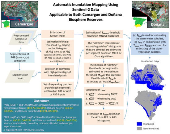
Automatic Inundation Mapping Using Sentinel-2 Data Applicable to Both Camargue and Doñana Biosphere Reserves


Abstract
1. Introduction
2. Materials and Methods
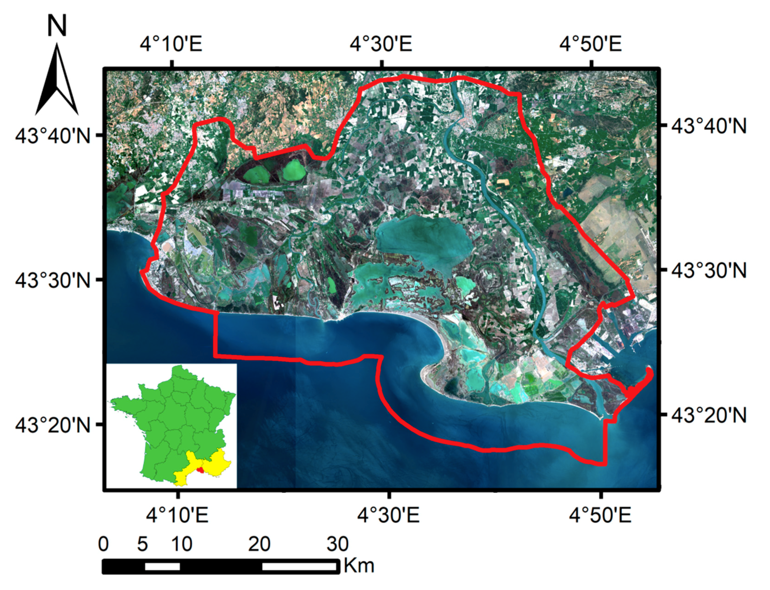
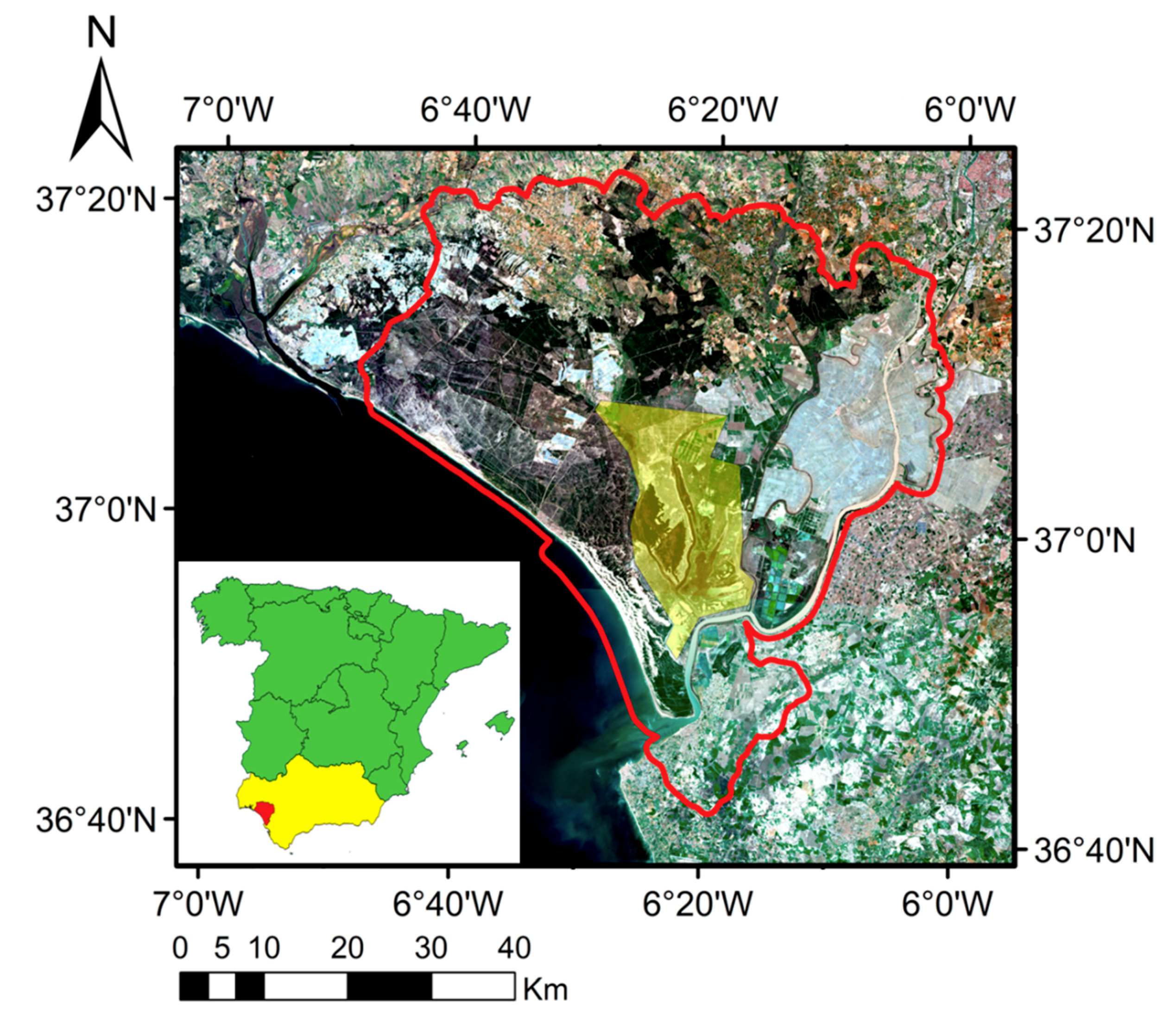
2.1. Study Areas
2.1.1. Camargue
2.1.2. Doñana
2.2. Dataset
2.2.1. Camargue
2.2.2. Doñana
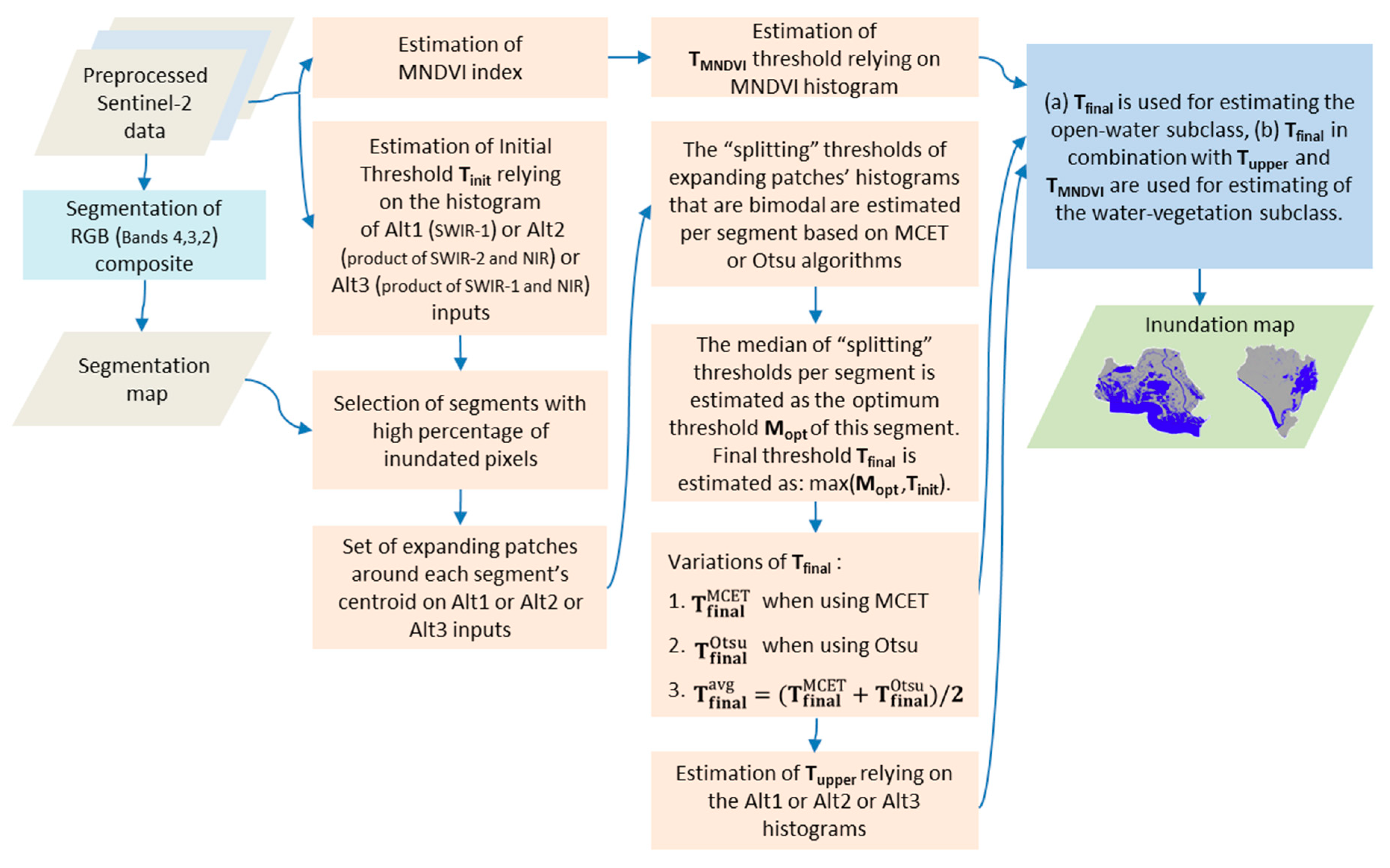
2.3. Methodology
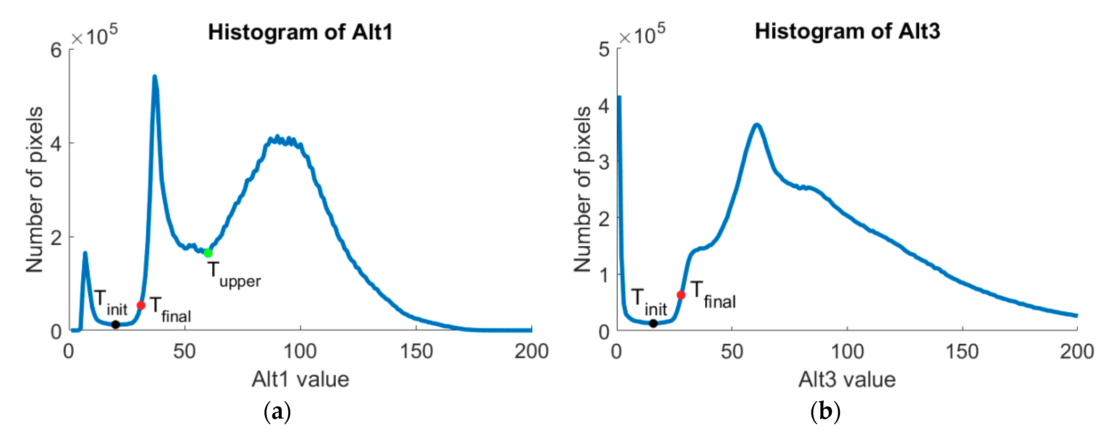
2.3.1. Segmentation of the Satellite Image
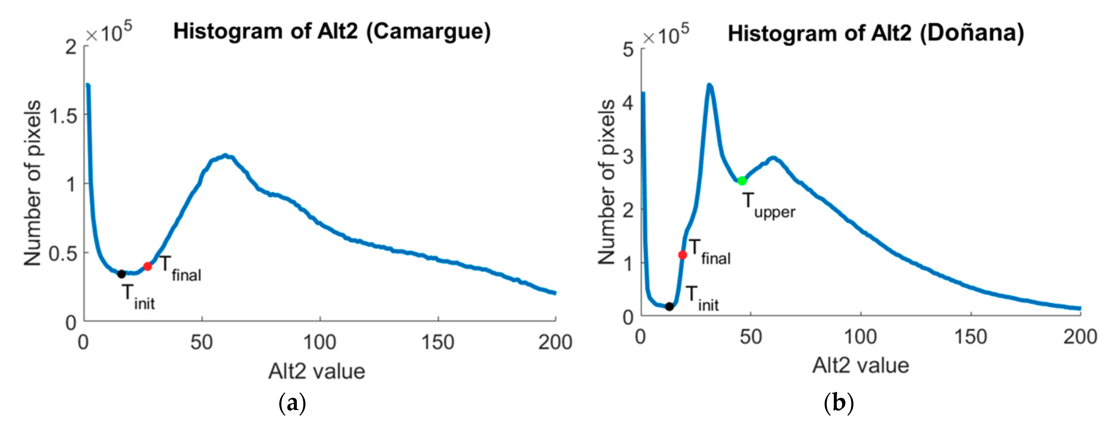
2.3.2. Mapping of the Open-Water Subclass
2.3.3. Mapping of the Water-Vegetation Subclass
3. Results
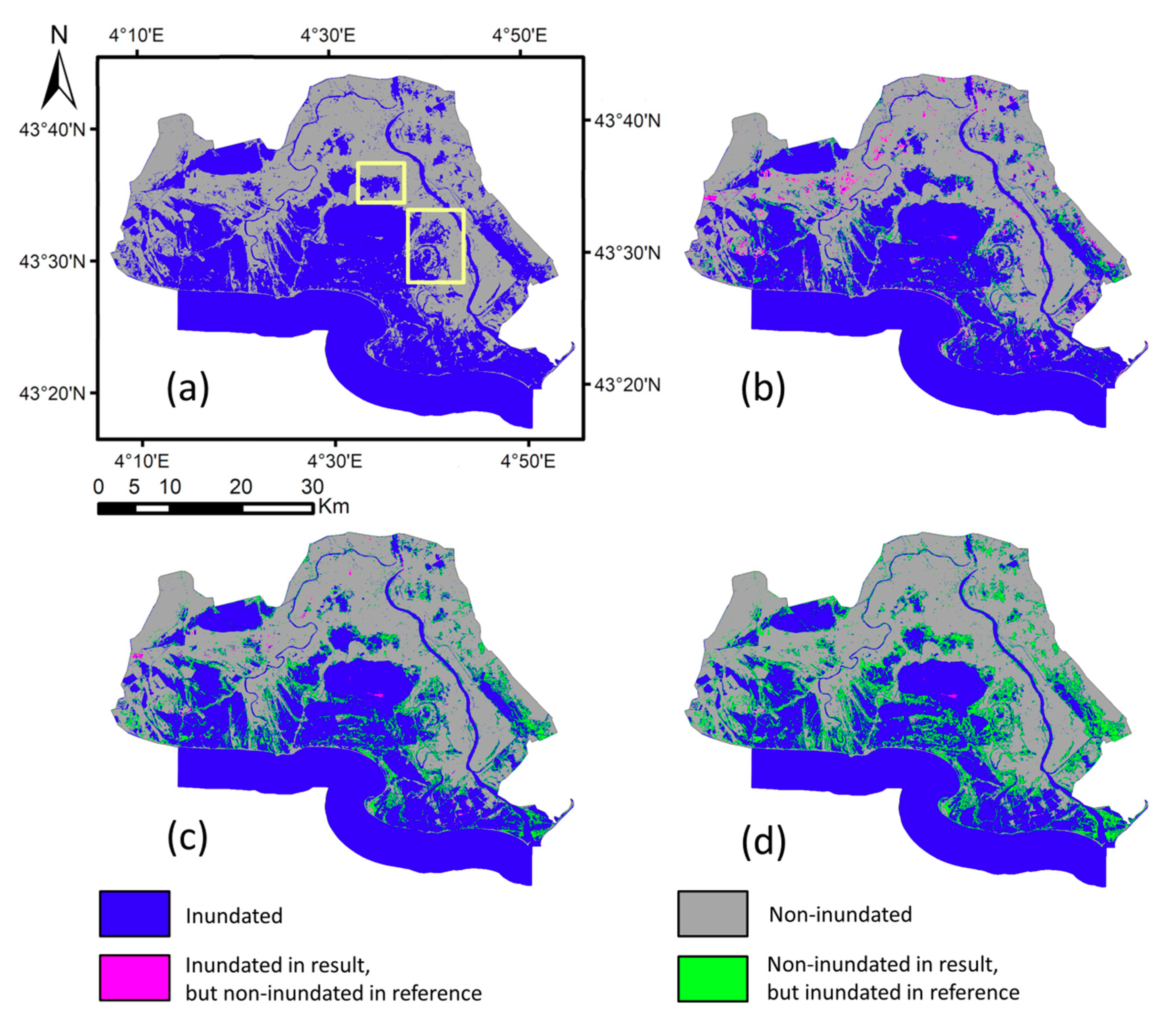
3.1. Comparison of Automatic Thresholding Results Against Reference Map of Camargue
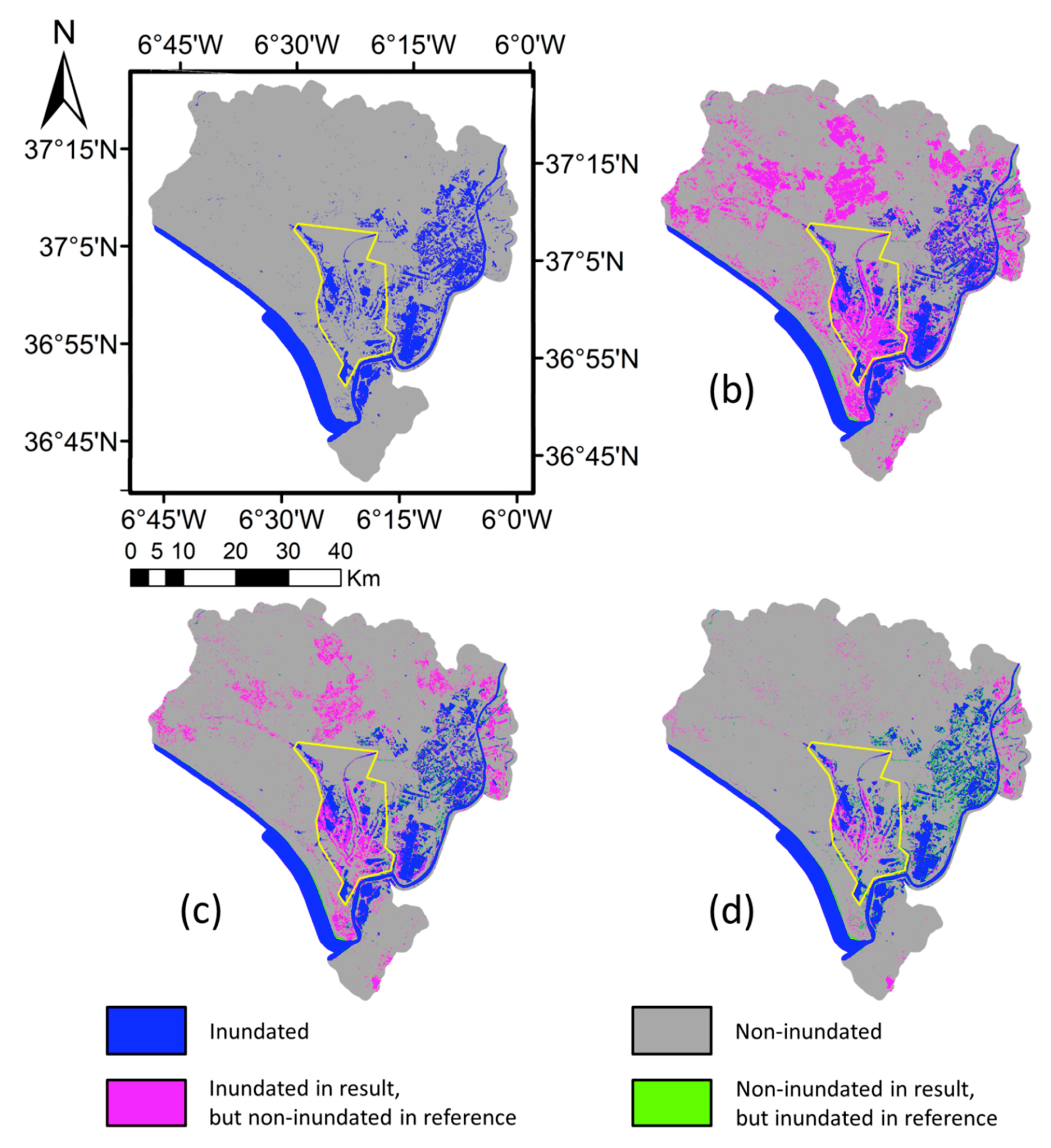
3.2. Comparison of Automatic and Thresholding Results Against Landsat Reference Maps of Doñana
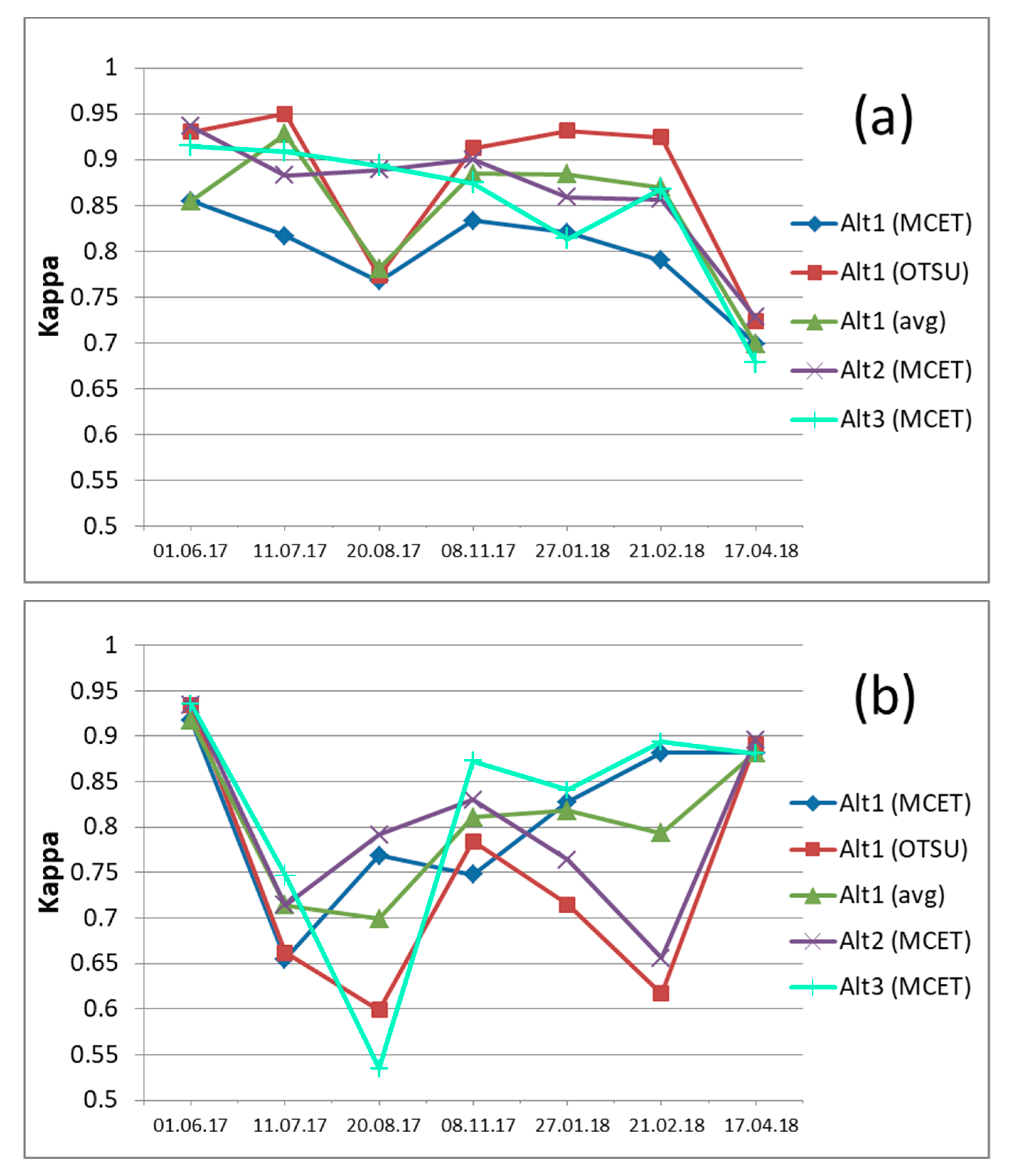
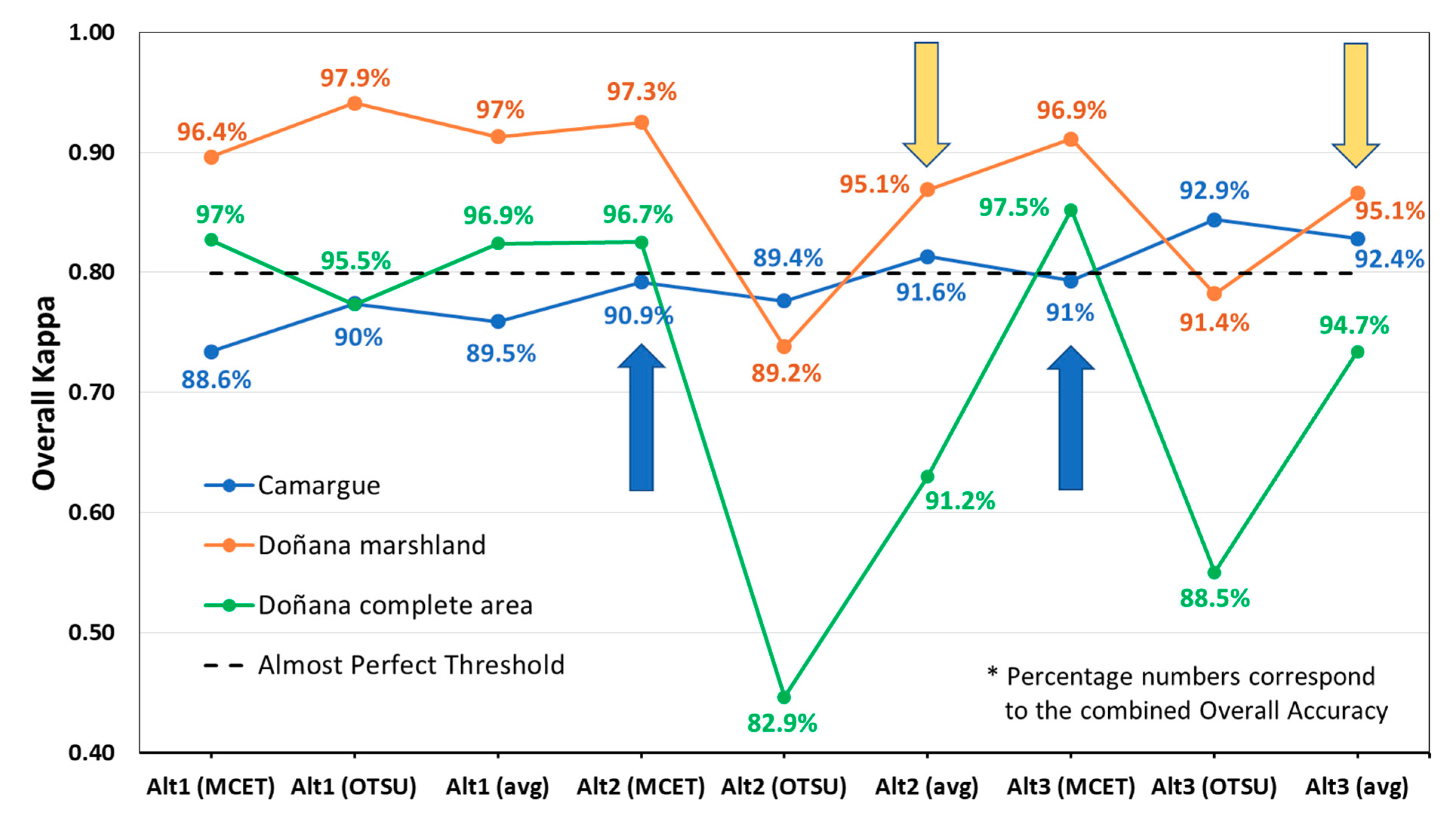
3.3. Overall Kappa Per Approach and Examined Areas
4. Discussion
5. Conclusions
Author Contributions
Funding
Acknowledgments
Conflicts of Interest
References
- World Resources Institute. Millennium Ecosystem Assessment: Ecosystems and Human Well-Being: Wetlands and Water Synthesis; World Resources Institute: Washington, DC, USA, 2005. [Google Scholar]
- Park, E.; Lee, S.; Peters, D.J. Iowa wetlands outdoor recreation visitors’ decision-making process: An extended model of goal-directed behavior. J. Outdoor Recreat. Tour. 2017, 17, 64–76. [Google Scholar] [CrossRef]
- Davidson, N.C. How much wetland has the world lost? Long-term and recent trends in global wetland area. Mar. Freshw. Res. 2014, 65, 934–941. [Google Scholar] [CrossRef]
- Huang, W.; DeVries, B.; Huang, C.; Lang, M.W.; Jones, J.W.; Creed, I.F.; Carroll, M.L. Automated Extraction of Surface Water Extent from Sentinel-1 Data. Remote Sens. 2018, 10, 797. [Google Scholar] [CrossRef]
- Töyrä, J.; Pietroniro, A. Towards operational monitoring of a northern wetland using geomatics-based techniques. Remote Sens. Environ. 2005, 97, 174–191. [Google Scholar] [CrossRef]
- Marti-Cardona, B.; Dolz-Ripolles, J.; Lopez-Martinez, C. Wetland inundation monitoring by the synergistic use of ENVISAT/ASAR imagery and ancilliary spatial data. Remote Sens. Environ. 2013, 139, 171–184. [Google Scholar] [CrossRef]
- Martinis, S.; Plank, S.; Ćwik, K. The use of Sentinel-1 time-series data to improve flood monitoring in arid areas. Remote Sens. 2018, 10, 583. [Google Scholar] [CrossRef]
- Giustarini, L.; Hostache, R.; Matgen, P.; Schumann, G.J.P.; Bates, P.D.; Mason, D.C. A change detection approach to flood mapping in urban areas using TerraSAR-X. IEEE Trans. Geosci. Remote Sens. 2012, 51, 2417–2430. [Google Scholar] [CrossRef]
- Schumann, G.; Di Baldassarre, G.; Bates, P.D. The utility of spaceborne radar to render flood inundation maps based on multialgorithm ensembles. IEEE Trans. Geosci. Remote Sens. 2009, 47, 2801–2807. [Google Scholar] [CrossRef]
- Shen, X.; Wang, D.; Mao, K.; Anagnostou, E.; Hong, Y. Inundation Extent Mapping by Synthetic Aperture Radar: A Review. Remote Sens. 2019, 11, 879. [Google Scholar] [CrossRef]
- Markert, K.N.; Chishtie, F.; Anderson, E.R.; Saah, D.; Griffin, R.E. On the merging of optical and SAR satellite imagery for surface water mapping applications. Results Phys. 2018, 9, 275–277. [Google Scholar] [CrossRef]
- Manakos, I.; Kordelas, G.A.; Marini, K. Fusion of Sentinel-1 data with Sentinel-2 products to overcome non-favourable atmospheric conditions for the delineation of inundation maps. Eur. J. Remote Sens. 2019, 1–14. [Google Scholar] [CrossRef]
- Davranche, A.; Poulin, B.; Lefebvre, G. Mapping flooding regimes in Camargue wetlands using seasonal multispectral data. Remote Sens. Environ. 2013, 138, 165–171. [Google Scholar] [CrossRef]
- Donchyts, G.; Schellekens, J.; Winsemius, H.; Eisemann, E.; van de Giesen, N. A 30 m resolution surface water mask including estimation of positional and thematic differences using landsat 8, srtm and openstreetmap: A case study in the Murray-Darling Basin, Australia. Remote Sens. 2016, 8, 386. [Google Scholar] [CrossRef]
- Du, Y.; Zhang, Y.; Ling, F.; Wang, Q.; Li, W.; Li, X. Water bodies’ mapping from Sentinel-2 imagery with modified normalized difference water index at 10-m spatial resolution produced by sharpening the SWIR band. Remote Sens. 2016, 8, 354. [Google Scholar] [CrossRef]
- Kyriou, A.; Nikolakopoulos, K. Flood mapping from Sentinel-1 and Landsat-8 data: A case study from river Evros, Greece. In Proc. SPIE 9644, Earth Resources and Environmental Remote Sensing/GIS Applications VI; International Society for Optics and Photonics: Toulouse, France, 2015; p. 964405. [Google Scholar] [CrossRef]
- Guo, Q.; Pu, R.; Li, J.; Cheng, J. A weighted normalized difference water index for water extraction using Landsat imagery. Int. J. Remote Sens. 2017, 38, 5430–5445. [Google Scholar] [CrossRef]
- Buma, W.; Lee, S.I.; Seo, J. Recent Surface Water Extent of Lake Chad from Multispectral Sensors and GRACE. Sensors 2018, 18, 2082. [Google Scholar] [CrossRef]
- Zhang, F.; Li, J.; Zhang, B.; Shen, Q.; Ye, H.; Wang, S.; Lu, Z. A simple automated dynamic threshold extraction method for the classification of large water bodies from landsat-8 OLI water index images. Int. J. Remote Sens. 2018, 39, 3429–3451. [Google Scholar] [CrossRef]
- Lee, K.S.; Kim, T.H.; Yun, Y.S.; Shin, S.M. Spectral characteristics of shallow turbid water near the shoreline on inter-tidal flat. Korean J. Remote Sens. 2001, 17, 131–139. [Google Scholar]
- Feyisa, G.L.; Meilby, H.; Fensholt, R.; Proud, S.R. Automated Water Extraction Index: A new technique for surface water mapping using Landsat imagery. Remote Sens. Environ. 2014, 140, 23–35. [Google Scholar] [CrossRef]
- Lefebvre, G.; Davranche, A.; Willm, L.; Campagna, J.; Redmond, L.; Merle, C.; Guelmami, A.; Poulin, B. Introducing WIW for detecting the presence of Water In Wetlands with Landsat and Sentinel satellites. Remote Sens. 2019, 11, 2210. [Google Scholar] [CrossRef]
- Kordelas, G.A.; Manakos, I.; Aragonés, D.; Díaz-Delgado, R.; Bustamante, J. Fast and Automatic Data-Driven Thresholding for Inundation Mapping with Sentinel-2 Data. Remote Sens. 2018, 10, 910. [Google Scholar] [CrossRef]
- Díaz-Delgado, R.; Aragonés, D.; Afán, I.; Bustamante, J. Long-term monitoring of the flooding regime and hydroperiod of Doñana marshes with Landsat time series (1974–2014). Remote Sens. 2016, 8, 775. [Google Scholar] [CrossRef]
- Bangira, T.; Alfieri, S.M.; Menenti, M.; van Niekerk, A. Comparing Thresholding with Machine Learning Classifiers for Mapping Complex Water. Remote Sens. 2019, 11, 1351. [Google Scholar] [CrossRef]
- Ban, H.J.; Kwon, Y.J.; Shin, H.; Ryu, H.S.; Hong, S. Flood monitoring using satellite-based RGB composite imagery and refractive index retrieval in visible and near-infrared bands. Remote Sens. 2017, 9, 313. [Google Scholar] [CrossRef]
- Chini, M.; Hostache, R.; Giustarini, L.; Matgen, P. A Hierarchical Split-Based Approach for Parametric Thresholding of SAR Images: Flood Inundation as a Test Case. IEEE Trans. Geosci. Remote Sens. 2017, 55, 6975–6988. [Google Scholar] [CrossRef]
- Otsu, N. A threshold selection method from gray-level histograms. IEEE Trans. Syst. Man Cybern. 1979, 9, 62–66. [Google Scholar] [CrossRef]
- Kittler, J.; Illingworth, J. Minimum error thresholding. Pattern Recognit. 1986, 19, 41–47. [Google Scholar] [CrossRef]
- Ko, B.C.; Kim, H.H.; Nam, J.Y. Classification of potential water bodies using Landsat 8 OLI and a combination of two boosted random forest classifiers. Sensors 2015, 15, 13763–13777. [Google Scholar] [CrossRef]
- DeVries, B.; Huang, C.; Lang, M.; Jones, J.; Huang, W.; Creed, I.; Carroll, M. Automated quantification of surface water inundation in wetlands using optical satellite imagery. Remote Sens. 2017, 9, 807. [Google Scholar] [CrossRef]
- Skakun, S. A neural network approach to flood mapping using satellite imagery. Comput. Inform. 2012, 29, 1013–1024. [Google Scholar]
- Nandi, I.; Srivastava, P.K.; Shah, K. Floodplain mapping through support vector machine and optical/infrared images from landsat 8 OLI/TIRS sensors: Case study from Varanasi. Water Resour. Manag. 2017, 31, 1157–1171. [Google Scholar] [CrossRef]
- Jakovljević, G.; Govedarica, M.; Álvarez-Taboada, F. Waterbody mapping: A comparison of remotely sensed and GIS open data sources. Int. J. Remote Sens. 2019, 40, 2936–2964. [Google Scholar] [CrossRef]
- Miao, Z.; Fu, K.; Sun, H.; Sun, X.; Yan, M. Automatic water-body segmentation from high-resolution satellite images via deep networks. IEEE Geosci. Remote Sens. Lett. 2018, 15, 602–606. [Google Scholar] [CrossRef]
- Isikdogan, F.; Bovik, A.C.; Passalacqua, P. Surface water mapping by deep learning. IEEE J. Sel. Top. Appl. Earth Obs. Remote Sens. 2017, 10, 4909–4918. [Google Scholar] [CrossRef]
- Acharya, T.; Lee, D.; Yang, I.; Lee, J. Identification of water bodies in a Landsat 8 OLI image using a J48 decision tree. Sensors 2016, 16, 1075. [Google Scholar] [CrossRef]
- Yousefi, P.; Jalab, H.A.; Ibrahim, R.W.; Noor, N.F.M.; Ayub, M.N.; Gani, A. Water-body segmentation in satellite imagery applying modified Kernel K-means. Malays. J. Comput. Sci. 2018, 31, 143–154. [Google Scholar] [CrossRef]
- Sivanpillai, R.; Miller, S.N. Improvements in mapping water bodies using ASTER data. Ecol. Inform. 2010, 5, 73–78. [Google Scholar] [CrossRef]
- Jiang, H.; Feng, M.; Zhu, Y.; Lu, N.; Huang, J.; Xiao, T. An automated method for extracting rivers and lakes from Landsat imagery. Remote Sens. 2014, 6, 5067–5089. [Google Scholar] [CrossRef]
- Zhou, Y.; Dong, J.; Xiao, X.; Xiao, T.; Yang, Z.; Zhao, G.; Zou, Z.; Qin, Y. Open Surface Water Mapping Algorithms: A Comparison of Water-Related Spectral Indices and Sensors. Water 2017, 9, 256. [Google Scholar] [CrossRef]
- Haibo, Y.; Zongmin, W.; Hongling, Z.; Yu, G. Water body extraction methods study based on RS and GIS. Procedia Environ. Sci. 2011, 10, 2619–2624. [Google Scholar] [CrossRef]
- Schwatke, C.; Scherer, D.; Dettmering, D. Automated Extraction of Consistent Time-Variable Water Surfaces of Lakes and Reservoirs Based on Landsat and Sentinel-2. Remote Sens. 2019, 11, 1010. [Google Scholar] [CrossRef]
- Chauvelon, P.; Tournoud, M.G.; Sandoz, A. Integrated hydrological modelling of a managed coastal Mediterranean wetland (Rhone delta, France): Initial calibration. Hydrol. Earth Syst. Sci. 2003, 7, 123–132. [Google Scholar] [CrossRef]
- Grillas, P. The Camargue: Rhone River Delta (France). In The Wetland Book: II: Distribution, Description and Conservation; Finlayson, C., Milton, G., Prentice, R., Davidson, N., Eds.; Springer: Dordrecht, The Netherlands, 2016. [Google Scholar]
- Lefebvre, G.; Germain, C.; Poulin, B. Contribution of rainfall vs. water management to Mediterranean wetland hydrology: Development of an interactive simulation tool to foster adaptation to climate variability. Environ. Model. Softw. 2015, 74, 39–47. [Google Scholar] [CrossRef]
- Lefebvre, G.; Redmond, L.; Germain, C.; Palazzi, E.; Terzago, S.; Willm, L.; Poulin, B. Predicting the vulnerability of seasonally-flooded wetlands to climate change across the Mediterranean Basin. Sci. Total Environ. 2019, 692, 546–555. [Google Scholar] [CrossRef] [PubMed]
- Martí-cardona, B. Spaceborne SAR Imagery for Monitoring the Inundation in the Doñana Wetlands. Ph.D. Dissertation, Polytechnic University of Catalonia, Barcelona, Catalonia, Spain, 2014. [Google Scholar]
- Green, A.J.; Bustamante, J.; Janss, G.F.E.; Fernández-Zamudio, R.; Díaz-Paniagua, C. Doñana Wetlands (Spain). In The Wetland Book: II: Distribution, Description and Conservation; Finlayson, C., Milton, G., Prentice, R., Davidson, N., Eds.; Springer: Dordrecht, The Netherlands, 2016. [Google Scholar]
- Kloskowski, J.; Green, A.J.; Polak, M.; Bustamante, J.; Krogulec, J. Complementary use of natural and artificial wetlands by waterbirds wintering in Doñana, south-west Spain. Aquat. Conserv. Mar. Freshw. Ecosyst. 2009, 19, 815–826. [Google Scholar] [CrossRef]
- Kullback, S. Information Theory and Statistics; Dover Publications: New York, NY, USA, 1968. [Google Scholar]
- Comaniciu, D.; Meer, P. Mean shift: A robust approach toward feature space analysis. IEEE Trans. Pattern Anal. Mach. Intell. 2002, 24, 603–619. [Google Scholar] [CrossRef]
- Landis, J.R.; Koch, G.G. The measurement of observer agreement for categorical data. Biometrics 1977, 33, 159–174. [Google Scholar] [CrossRef]
- Nakmuenwai, P.; Yamazaki, F.; Liu, W. Automated Extraction of Inundated Areas from Multi-Temporal Dual-Polarization RADARSAT-2 Images of the 2011 Central Thailand Flood. Remote Sens. 2017, 9, 78. [Google Scholar] [CrossRef]
- Martinis, S.; Kuenzer, C.; Wendleder, A.; Huth, J.; Twele, A.; Roth, A.; Dech, S. Comparing four operational SAR-based water and flood detection approaches. Int. J. Remote Sens. 2015, 36, 3519–3543. [Google Scholar] [CrossRef]
- Li, J.; Wang, S. An automatic method for mapping inland surface waterbodies with Radarsat-2 imagery. Int. J. Remote Sens. 2015, 36, 1367–1384. [Google Scholar] [CrossRef]
- Bioresita, F.; Puissant, A.; Stumpf, A.; Malet, J.P. A method for automatic and rapid mapping of water surfaces from sentinel-1 imagery. Remote Sens. 2018, 10, 217. [Google Scholar] [CrossRef]
- Bovolo, F.; Bruzzone, L. A split-based approach to unsupervised change detection in large-size multitemporal images: Application to tsunami-damage assessment. IEEE Trans. Geosci. Remote Sens. 2007, 45, 1658–1670. [Google Scholar] [CrossRef]
- Toral, G.M.; Aragones, D.; Bustamante, J.; Figuerola, J. Using Landsat images to map habitat availability for waterbirds in rice fields. Ibis 2011, 153, 684–694. [Google Scholar] [CrossRef]
- Padró, J.-C.; Pons, X.; Aragonés, D.; Díaz-Delgado, R.; García, D.; Bustamante, J.; Pesquer, L.; Domingo-Marimon, C.; González-Guerrero, Ò.; Cristóbal, J.; et al. Radiometric correction of simultaneously acquired Landsat-7/Landsat-8 and Sentinel-2A imagery using pseudoinvariant areas (PIA): Contributing to the Landsat time series legacy. Remote Sens. 2017, 9, 1319. [Google Scholar] [CrossRef]
- Martins, V.; Barbosa, C.; de Carvalho, L.; Jorge, D.; Lobo, F.; Novo, E. Assessment of atmospheric correction methods for Sentinel-2 MSI images applied to Amazon floodplain lakes. Remote Sens. 2017, 9, 322. [Google Scholar] [CrossRef]


| Cycle | Sept. | Oct. | Nov. | Dec. | Jan. | Feb. | Mar. | Apr. | May | June | July | Aug. |
|---|---|---|---|---|---|---|---|---|---|---|---|---|
| 2016–2017 | 12,19 | 4,7 12,14 17 | 3,13 18,21 | |||||||||
| 2017–2018 | 5,7 20,27 | 5,7 10,12 27,30 | 14,16 19,21 | 6,9 16,24 | 23 | 4,22 27 | 14 | 18,20 | 20,25 | 19 |
| Date | 01/06/2017 | 11/07/2017 | 20/08/2017 | 08/11/2017 | 27/01/2018 | 21/02/2018 | 17/04/2018 |
© 2019 by the authors. Licensee MDPI, Basel, Switzerland. This article is an open access article distributed under the terms and conditions of the Creative Commons Attribution (CC BY) license (http://creativecommons.org/licenses/by/4.0/).
Share and Cite
Kordelas, G.A.; Manakos, I.; Lefebvre, G.; Poulin, B. Automatic Inundation Mapping Using Sentinel-2 Data Applicable to Both Camargue and Doñana Biosphere Reserves. Remote Sens. 2019, 11, 2251. https://doi.org/10.3390/rs11192251
Kordelas GA, Manakos I, Lefebvre G, Poulin B. Automatic Inundation Mapping Using Sentinel-2 Data Applicable to Both Camargue and Doñana Biosphere Reserves. Remote Sensing. 2019; 11(19):2251. https://doi.org/10.3390/rs11192251
Chicago/Turabian StyleKordelas, Georgios A., Ioannis Manakos, Gaëtan Lefebvre, and Brigitte Poulin. 2019. "Automatic Inundation Mapping Using Sentinel-2 Data Applicable to Both Camargue and Doñana Biosphere Reserves" Remote Sensing 11, no. 19: 2251. https://doi.org/10.3390/rs11192251
APA StyleKordelas, G. A., Manakos, I., Lefebvre, G., & Poulin, B. (2019). Automatic Inundation Mapping Using Sentinel-2 Data Applicable to Both Camargue and Doñana Biosphere Reserves. Remote Sensing, 11(19), 2251. https://doi.org/10.3390/rs11192251