Article

Investigating the Impact of Land Parcelization on Forest Composition and Structure in Southeastern Ohio Using Multi-Source Remotely Sensed Data

1
Department of Land Surveying and Geo-Informatics, The Hong Kong Polytechnic University, Kowloon, Hong Kong
2
Department of Geography, The Ohio State University, Columbus, OH 43210, USA
*
Author to whom correspondence should be addressed.
Remote Sens. 2019, 11(19), 2195; https://doi.org/10.3390/rs11192195
Submission received: 7 August 2019 / Revised: 13 September 2019 / Accepted: 18 September 2019 / Published: 20 September 2019
(This article belongs to the Special Issue Forest Degradation Monitoring)

Abstract

:
Forestland parcelization (i.e., a process by which large parcels of forestland ownership are divided into many small parcels) presents an increasing challenge to sustainable forest development in the United States. In Southeastern Ohio, forests also experienced intensive forestland parcelization, where the majority of forest owners own parcels smaller than 10 acres currently. To better understand the impact of forestland parcelization on forest development, this study employed multi-source remotely sensed data and land ownership data in Hocking County, Ohio to examine the relationship between forestland parcel size and forest attributes, including forest composition and structure. Our results show that private forestland parcels are generally smaller than public forestland (the average parcel sizes are 21.5 vs. 275.0 acres). Compared with private lands, public lands have higher values in all forest attributes, including forest coverage, abundance of oak-dominant stands, canopy height and aboveground biomass. A further investigation focusing on private forestland reveals that smaller parcels tend to have smaller forest coverage, less greenness, lower height and aboveground biomass, indicating that forests in smaller parcels may experience more human disturbances than larger parcels. The results also show that logarithmic models can well quantify the non-linear relationship between forest attributes and parcel size in the study area. Our study suggests that forestland parcelization indeed has negative effects on forest development, so it is very important to take appropriate measures to protect forests in small ownership parcels.

Graphical Abstract

1. Introduction

According to the global land cover map derived from Landsat images [1], forests cover 28.35% of the world. In the United States, about 36% of the land area, or 816 million acres, is forest land [2]. The forest of the United States has been well protected from clearing for agriculture, settlement, and other uses since the 1920s [3]. However, speeding-up forestland parcelization, defined as the subdivision of forest land holdings into smaller ownership parcels [4], is currently challenging sustainable forest development, especially for 49% of the national forestlands owned by non-industrial private forest (NIPF) owners [5]. Forestland parcelization increases the number of forest landowners while decreasing the average size of parcels [6]. The increasing rate of forestland parcelization may be driven by economic and demographic factors, such as death, urbanization, and income structure [5,6]. Forestland parcelization is a national trend. This seriously affects Southeastern Ohio where 85% of the forestland is privately owned, and the majority of owners hold less than 10 acres.
Understanding the impact of forestland parcelization is fundamental to forest management and conservation. Through field survey, field experiments, national or local inventory data, and landowner interviews, studies have suggested that the increasing forest parcelization has various implications for the ecosystem and socioeconomic systems [7,8,9]. The implications may include: leading to forest fragmentation from a landscape perspective [10], changing the composition and structure of forest [5], altering the original habitat conditions, connectivity and the microenvironment [11], impacting many forest-derived goods and services [4], threatening the timber products industry, diminishing economies of scale, reducing public access to forested lands for outdoor recreation, and challenging the sustainable forest management [12].
However, existing studies of forestland parcelization using traditional approaches have some limitations. First, field work is very time consuming, costly, and requires observers with adequate technical expertise [13]. For example, a field survey in Brazilian forest costs 145,550 dollars and 18,200 person-hours for recording 60,393 trees [14]. Second, due to budgetary constraints and difficulties to access remote forests, it is impossible to complete surveys at all the locations on forestlands. Therefore, conclusions drawn from field survey may be biased [15]. Although various sampling designs have been used to improve the efficiency and representativeness, bias between estimated values by samples and ground truth still exists. Third, sample based results do not provide enough spatially explicit details. In contrast, remotely sensed data makes the inventories with low cost [16] and covers all the locations in an area [15] compared with the traditional approaches for forest inventory. Both active and passive remotely sensed data can achieve promising results for mapping forest composition and estimating structural parameters. For example, Landsat images were used to map global forest cover with 93% accuracy [17] and model forest characteristics in Georgia, USA with accuracy higher than 80% [18]. Airborne LiDAR data were successfully used to estimate forest attributes, such as tree height [19] and growing stock volume [20]. However, to the best of our knowledge, studies of forest parcelization using remote sensing technology are very limited. A recent study used multi-year Landsat images to identify harvesting events for private forests in Michigan from 1985 to 2011 [21]. Third, most of the existing studies focus on highly parcelized forests or compare forests separated by long spatial distance [9,22,23]. As a result, it is not very convincing to conclude that forest parcellization has brought negative effects on forest development without direct comparison between forests with small and large parcels under the similar environmental conditions. To control for the confounding factors of environmental conditions, including climate and soil, on the comparison [24,25], the forests with different parcel sizes should be spatially adjacent within a relatively homogenous area.
To overcome the above-mentioned limitations of existing studies, this paper investigates the impact of land ownership parcel sizes on forest composition and structure in Southeastern Ohio using multi-source remotely sensed data. The first objective is to map forest composition and structure using the cutting-edge remote sensing technologies. Considering that passive and active remote sensing data complement each other in forest monitoring, this study makes full use of the strengths of different types of remotely sensed data. The second objective is to reveal how forest parcelization affects the forest development through comparing forests in the private and public lands and analyzing the relationship between forest attributes and parcel size. In the selected study area, the public land parcels are much larger than those of private holdings, which enables us to directly compare the forest composition and structure of parcelized forest and non-parcelized forest under the similar environmental conditions. The rest of the paper is organized as follows. Section 2 presents the study area and data sets. Section 3 describes the approaches for mapping forest attributes and the statistical analysis involved. Section 4 shows the results and Section 5 discusses the possible ways in which parcelization affects forest development. Section 6 concludes this study.

2. Study Area and Data
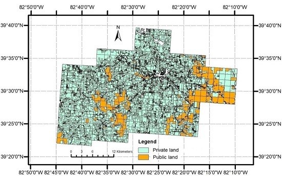
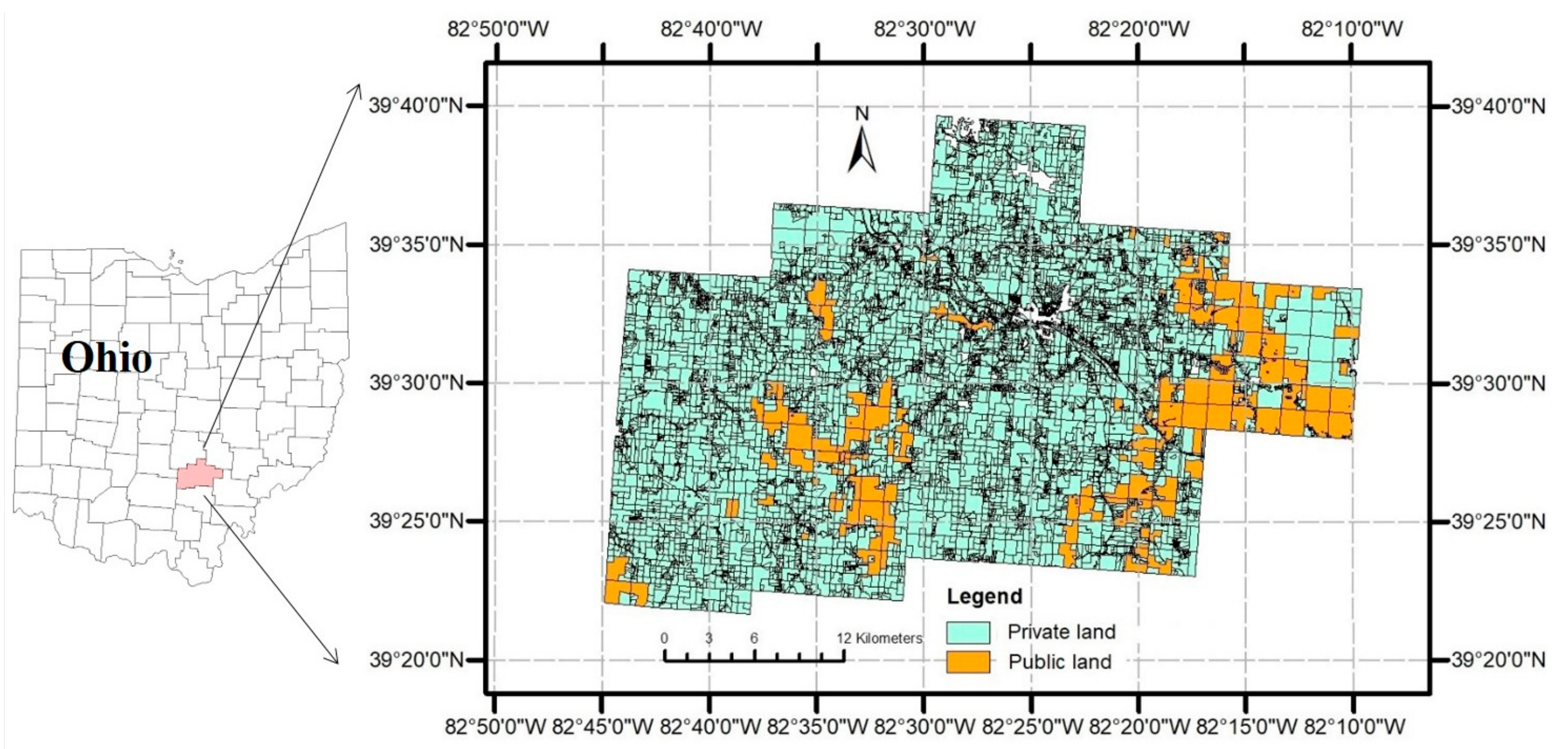
2.1. Study Area

The study area is Hocking County in Southeastern Ohio (Figure 1). The study area covers approximately 1098 km2. The major land cover is forests. The original forests (old-growth) in this area were cut or burned one or more times for agriculture and to fuel both industry and farm homes. The vegetation types before European settlement in 1788 (pre-settlement) were mixed-oak, mixed-mesophytic, and beech forests [26]. The second-growth forests in this region were heavily disturbed by the harvesting of timber, coal mining, and animal grazing. Now, the major forest types are oak-hickory and mixed-hardwood [27]. Abundant tree species include white oak, black oak, yellow poplar, hickory, sugar maple, red maple, ash, pine, chestnut oak, scarlet oak and beech according to forest inventory and analysis (FIA) data. The study area is composed of both private (85.4%) and public lands (14.6%). One of the largest public lands is the Hocking Hills State Park. The public lands are well-managed to create large, continuous blocks of forest, while the surrounding private lands are increasingly parcelized under the pressure of population increase and commercial and industrial development in the area [28]. Therefore, the selected study area represents an ideal laboratory to study forest parcelization through direct comparison between two types of ownership.

2.2. Data

The data used in this study include land ownership map, Landsat imagery, and airborne LiDAR data. The land ownership map is a digital GIS file which records the ownership of each land parcel as a polygon. This map was provided by the Hocking County Mapping Department. The land ownership in this dataset was collected around year 2010. It recorded small parcels (e.g., lands occupied by individual houses) to large (e.g., the state parks). All small parcels with area < 1 acre were excluded from our analysis as trees were rarely planted in tiny parcels [29]. All parcels with area > 1 acre were summarized in Table 1. The average parcel size of private lands is much smaller than that of public lands (21.5 acres vs. 275 acres).
Six cloud-free Landsat TM images were collected in different seasons during 2007 and 2008 (April 17, 2007, June 6, 2008, June 20, 2007, September 10, 2008, September 24, 2007, and October 8, 2008). Images were collected during a two-year period because cloud-free images in one year could not cover all seasons and we assume that forests within a two-year period have minimal disturbances. These Landsat images covering the entire growing season of trees have higher capacity for mapping tree species and modeling forest biophysical attributes than an individual image [30,31]. These Landsat images were leavel-1 terrain corrected (L1T) products downloaded from the United States Geological Survey (USGS) EarthExplorer (http://earthexplorer.usgs.gov/). These images were then calibrated into top-of-atmosphere reflectance using the solar angles and calibration coefficients in their header files. Because there is hilly terrain within the study area, the Landsat images were further topographically corrected by the classic C-correction method to remove the illumination differences on steep terrains [32]. These Landsat images were used to map land cover and forest types in the study area and model the forest attributes including greenness and aboveground biomass. The details are explained in the Method section.
The airborne LiDAR covering the Hocking County was provided by the Ohio Statewide Imagery Program (OSIP). The OSIP is a partnership between State agencies and the federal government to develop high-resolution imagery and elevation data for the entire state to benefit GIS users at all levels of government. The LiDAR data used in this study was 2 m first and last returns LAS format archived by County which was downloaded from the OSIP website (https://ogrip.oit.ohio.gov/). The data was collected in 2007 under leaf-off condition which can be used to estimate tree attributes with satisfactory accuracy [33]. This LiDAR dataset was used to map the tree heights and stem density.
The ancillary datasets include a SRTM DEM data downloaded from USGS EarthExplorer and ground plot data provided by the Ohio Department of Natural Resources and USDA Forest Service. The SRTM DEM was resampled to 30 m to match the resolution of Landsat images. It was used to assist the topographic correction of Landsat images and provide topographic features for mapping the forest types. The group plot data provide the ground reference data for training and validating the models for forest mapping and biophysical attribute modelling.

3. Methods

Figure 2 shows the flowchart of this study. Steps are detailed in the following sections.

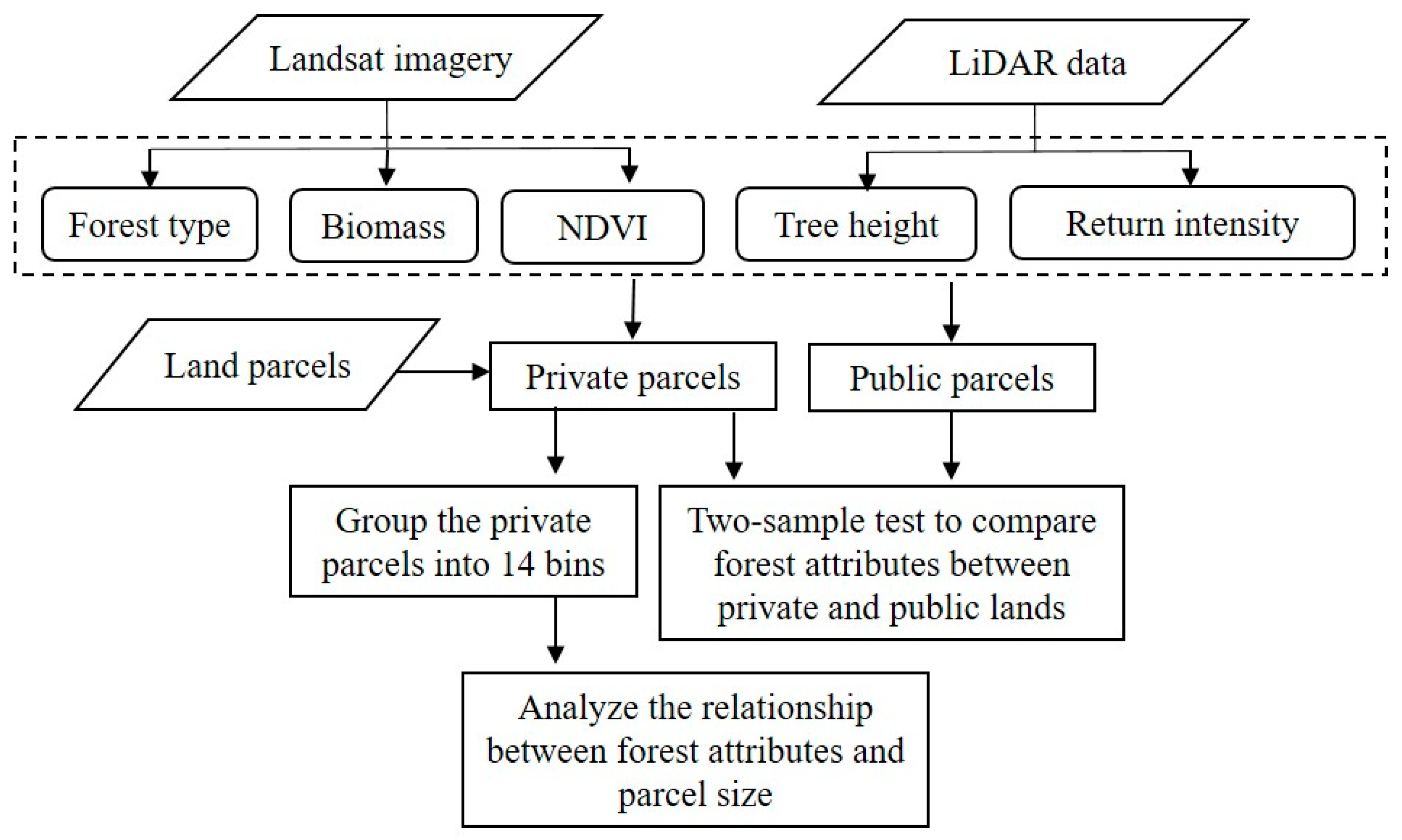
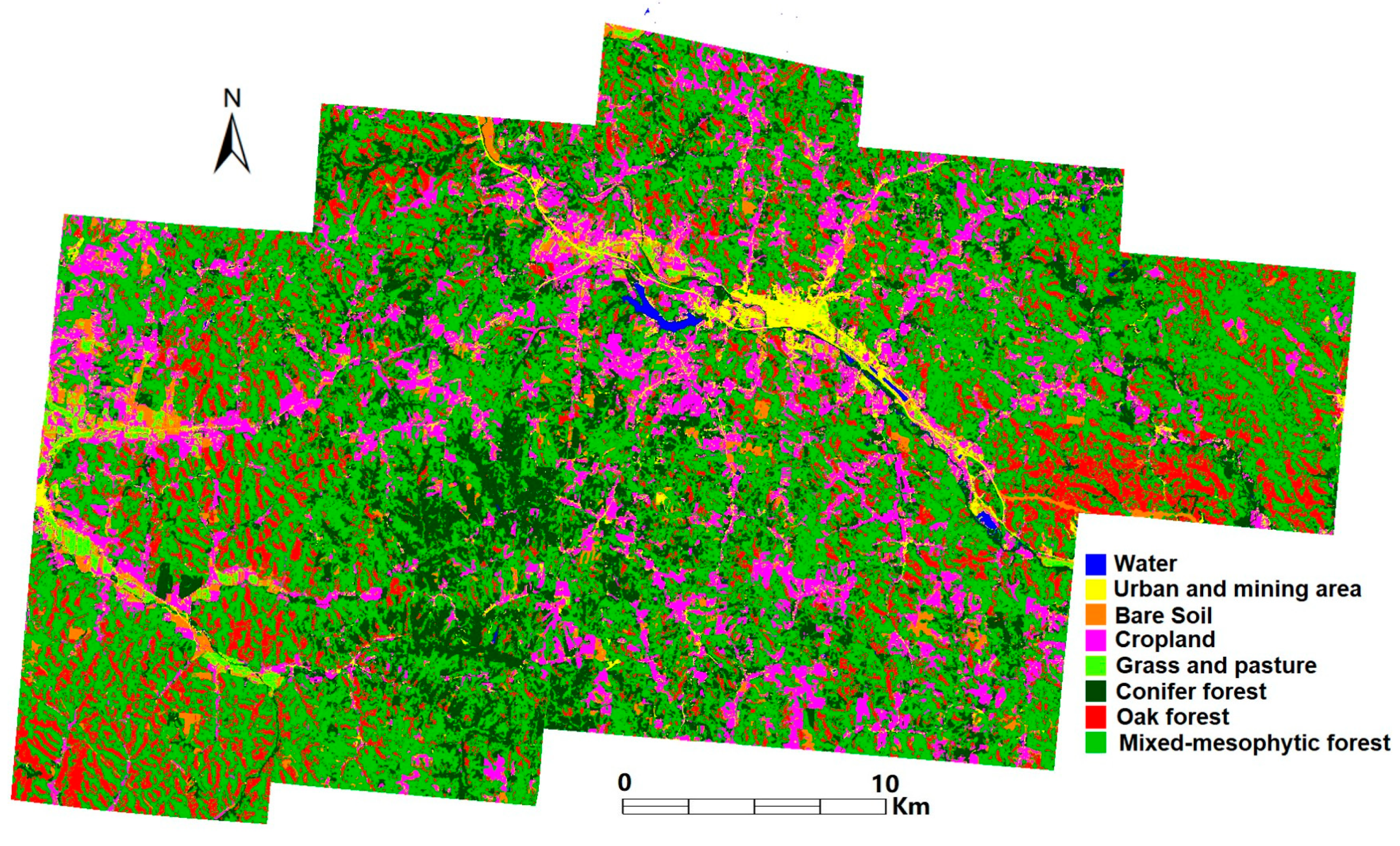
3.1. Mapping Forest Attributes

Landsat time series was used to map the forest types, greenness, and aboveground biomass. In our previous studies, a hierarchical method was developed to get detailed forest types from dense Landsat time-series and DEM data [31]. This hierarchical classification method classifies images into major land cover types in the first hierarchy and then classifies the forest class into more detailed forest types in the second hierarchy. It integrates a feature selection and a training-sample-adding procedure in the second hierarchy to improve classification accuracy. The accuracy of the proposed method has been assessed by error matrix using ground reference data (95 plots) collected in Southeastern Ohio. The overall accuracy, users’ and producers’ accuracy of forest type mapping reach 90% [31], demonstrating that the method is capable of obtaining reliable results. This method trained by ground samples was used to map forest types in Hocking County. Specifically, besides the five non-forest land cover types (water, urban build-up, bare land, cropland, grassland), forests were classified into three major types: pine forest, oak forest, and mixed-mesophytic forest (i.e., maple/beech/birch group) as shown in Figure 3. This classification scheme considers the importance of oak forest for both ecological and economic systems in the study area. Oak forests provide food and habitat for wildlife and support the local timber industry. However, the abundance of oak trees has declined in recent decades [34]. It is necessary to investigate the presence of oak trees in forestlands with different parcel sizes.
Normalized difference vegetation index (NDVI) is a widely used spectral index for describing the greenness of vegetation. NDVI is the normalized reflectance difference between the near infrared and the red bands. Considering that NDVI saturates in dense canopies [35], NDVI values derived from two Landsat images, one image of June 20, 2017 representing the peak season (Figure 4) and another one of September 24, 2007 representing descending season (image not shown), were used to investigate the forest greenness in parcels with different sizes.
The forest aboveground biomass (AGB) was estimated using Landsat NDVI time series and artificial neural network (ANN) method. Our previous study explored the use of seasonal NDVI time series derived from Landsat images across different seasons to estimate AGB in Southeastern Ohio by six empirical modeling approaches, including simple linear regression, stepwise multiple linear regression, partial least squares regression, reduced major axis regression, random forest regression, and ANN regression [30]. Results clearly show that NDVI in the fall season has a stronger correlation to AGB than the peak season. Furthermore, using seasonal NDVI time series can obtain more accurate AGB estimates and less saturation problem than using a single NDVI. From the comparison of these six empirical methods, it is difficult to decide which is superior because they have different strengths and their accuracy is generally similar. In this study, ANN model was chosen for mapping AGB in the study area because ANN obtained smaller root-mean-square error (RMSE) than other methods in the validation data in Southeastern Ohio (RMSE = 37.31 ton/ha, R2 = 0.54) [30]. The AGB map of our study area was shown in Figure 5.
The canopy height was estimated from LiDAR data by using an open-source tool LAStools (obtained from http://rapidlasso.com/LAStools). LAStools provides a series of tools for converting, filtering, viewing, gridding, and compressing of the raw LiDAR data. Four steps were processed for generating tree height map in the study area: 1) use “lasground” tool to classify the raw LiDAR points into ground points and non-ground points; 2) use “Lasheight” tool to extract the height of each point above the ground; 3) use “Lascanopy” tool to generate tree height at 2 m grid; and 4) resample the 2 m grid tree height map to 30 m to match the spatial resolution of Landsat images, i.e., in each 30 m grid, calculate the average of all 2 m grids with height > 2 m assuming that grids with height < 2 m do not have trees or only have small saplings. The 30 m tree height map is shown in Figure 6. For each 30 m grid, we also computed average intensity of returns. In leaf-off situation, backscattering intensity of LiDAR points hitting stems or branches is lower than bare ground and other green vegetation, so lower values of LiDAR intensity in winter could show higher stem volume [33]. Figure 7 shows that the low values in intensity well match the pixels with high forest density (i.e., the dark green pixels) in the summer Landsat image.

3.2. Statistical Analysis

We first summarized the pixel-wise values of forest attributes into each land parcel. Based on all 30 m pixels within each parcel (the smallest parcel covers about 4 pixels), the forest coverage (i.e., the percent of forest pixels in each parcel) and percent of other non-vegetation covers can be computed. In each parcel, only forest pixels were used to derive the percent of oak trees, average biomass, average NDVI, average tree height, and average LiDAR pulse return intensity.
We then compared forest composition and structural attributes between private and public parcels using two-sample t-test. The null hypothesis is that means of forest attributes of two groups (i.e., private and public parcels) are equal in all aspects, including abundance of oak trees, AGB, tree height, greenness, and stem volume. The alternative hypothesis is defined based on our prior knowledge. For example, many previous studies found that forest coverage is lower in private lands than that in public lands, so the alternative hypothesis of forest coverage is that the mean forest coverage in public lands is larger than that in private lands. The test statistic, t value, was then computed by using the mean and standard deviation of the two groups. Last, the P-value can be obtained by checking the t-distribution table. The two groups are significantly different if P-value is lower than 0.05.
We further analyzed the relationship between forest attributes and parcel size by only using private parcels because there are much more private parcels than public parcels and private parcels have larger variability in size than public parcels (Table 1). In addition, forestland parcelization often happens in private land rather than public land, so investigating how the size of private forestland affects the forest attributes can help to predict the future scenario if the forestland parcelization continues. To delineate this effect, we adopted a bin-based strategy. First, we divided private parcels into 14 bins with different size ranges (Figure 8). Here, unequal bins were used to ensure that each bin has sufficient number of parcels because the number of parcels generally dramatically decreases with size. Second, we summarized the forest attributes in each bin as the mean value and percentiles. Third, we plotted each forest attribute versus parcel size. Last, we assessed how the forest attributes change with the parcel size and modeled this relationship by regression analysis. The bin-based strategy is widely used to explore the relationship between two variables with large samples because it can clearly show the pattern from the messy sample points and meanwhile reduce the effect of outliers. For example, a study analyzed how the vegetation greenness changes with elevation through dividing the elevation range into bins with 100 m interval [36]. Serval private parcels with areas larger than 200 acres were excluded from this analysis because they have very similar forest attributes with parcels in the range 150–200 acres.

4. Results

4.1. Comparison between Parcelized Private Lands and Intact Public Lands

Table 2 lists the t-test results of various forest attributes between private and public lands. We can see that all the alternative hypotheses should be accepted because all the P-values are smaller than 0.0001. The forest coverage, peak-season NDVI, fall-season NDVI, tree height and aboveground biomass of public lands are significantly larger than those of private lands, and LiDAR intensity of public lands is significantly lower than private lands. All these t-test results suggest that forests in public lands are older and denser than those in private lands.

4.2. Relationship between Forest Attributes and Parcel Sizes of Private Lands

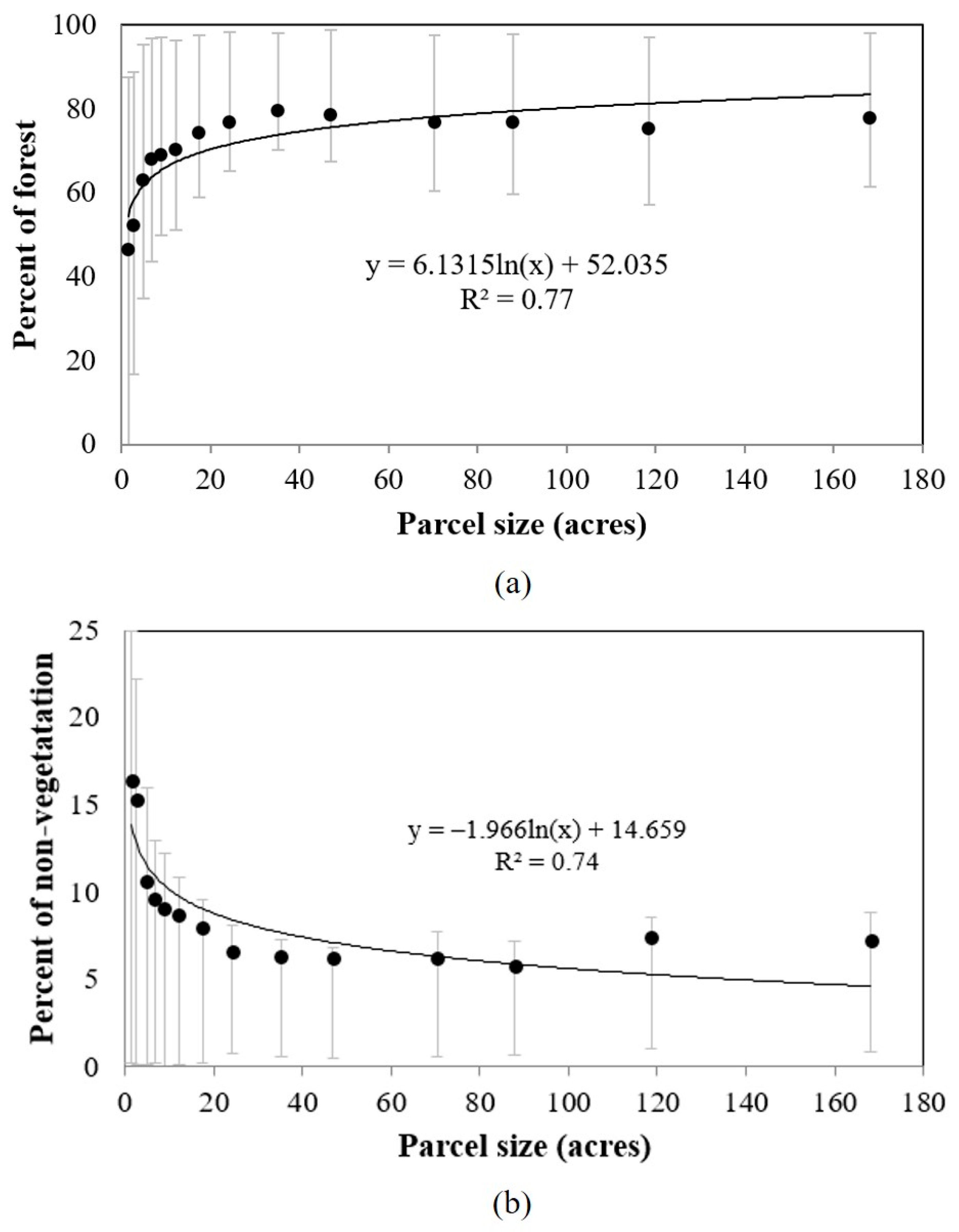
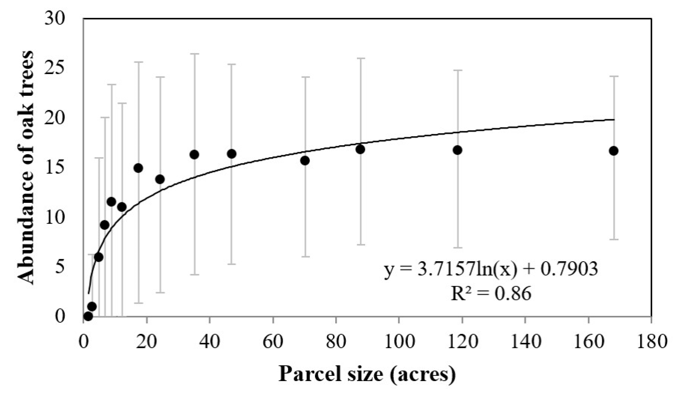
4.2.1. Forest Coverage and Abundance of Oak Trees

Figure 9 shows the percent of forest coverage and percent of non-vegetation versus parcel size. From Figure 9, we can see that (1) larger parcels have larger forest coverage and smaller within-group variance; (2) more lands were used for non-vegetation (e.g., construction and farming) in smaller parcels; (3) parcels of 1–10 acres have large variance in percentage of non-vegetation land cover; (4) when parcels >30 acres, the percentage of both forests and non-vegetation becomes relatively stable, i.e., the mean percentage of forests reach 80% and the non-vegetation covers are about 7%; and (5) logarithmic regression can well model the non-linear relationship of both forest coverage and non-vegetation fraction against parcel size (R2 values are 0.77 and 0.74 respectively). The logarithmic model suggests that the forest coverage increases (non-vegetation fraction decreases) rapidly at small parcels but then the change steadily slows as parcel size increases.
Figure 10 shows that the abundance of oak trees (i.e., the ratio of oak-dominated forest over total forest cover in each parcel) increases with parcel size. The mean value of oak tree abundance becomes stable around 15% when parcel size is larger than 30 acres. In addition, the range of oak tree abundance in each bin is large, suggesting that land parcels with similar size have very different oak tree abundance. The relationship between oak-tree abundance and parcel size can be also modeled by the logarithmic regression (R2: 0.86).

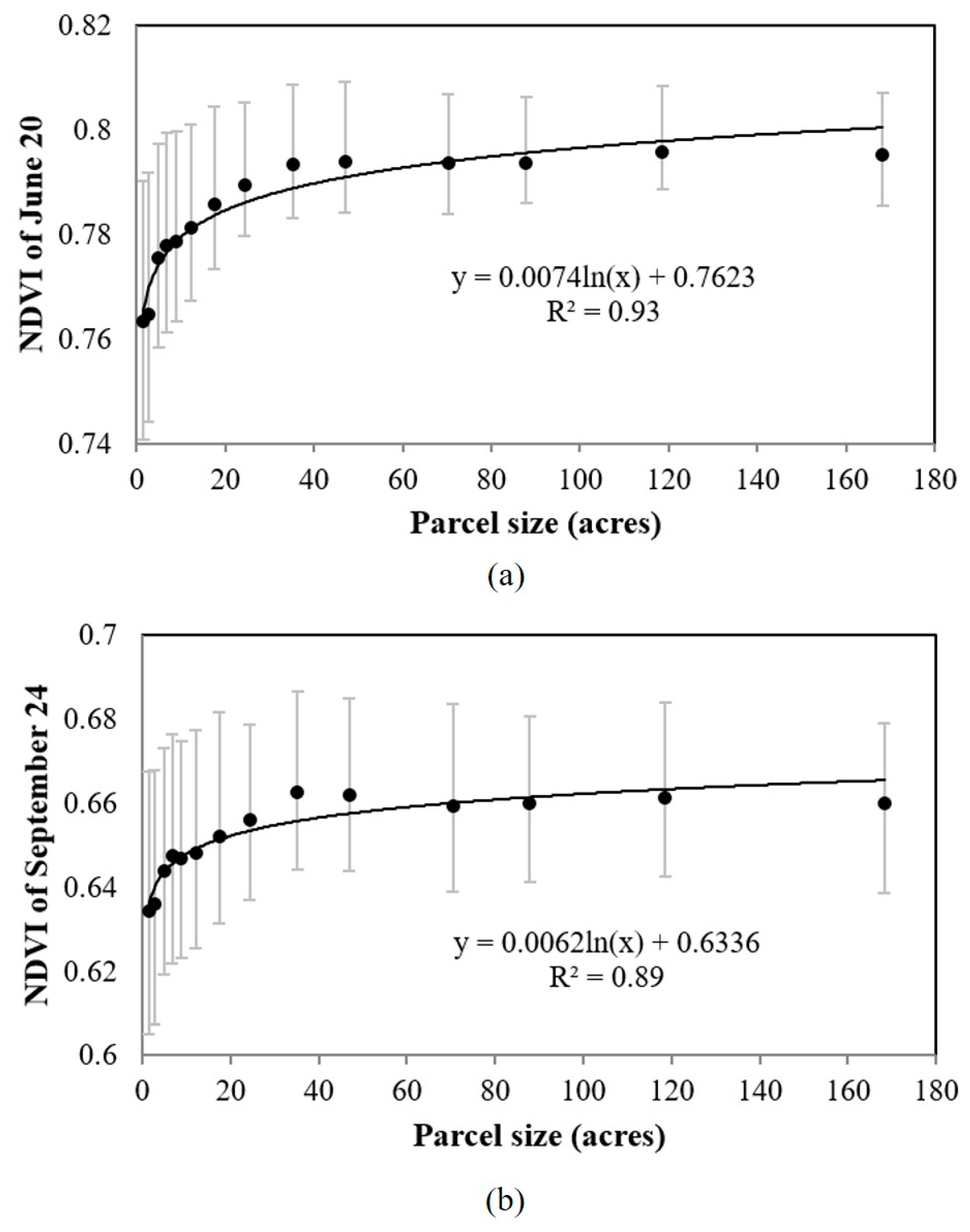
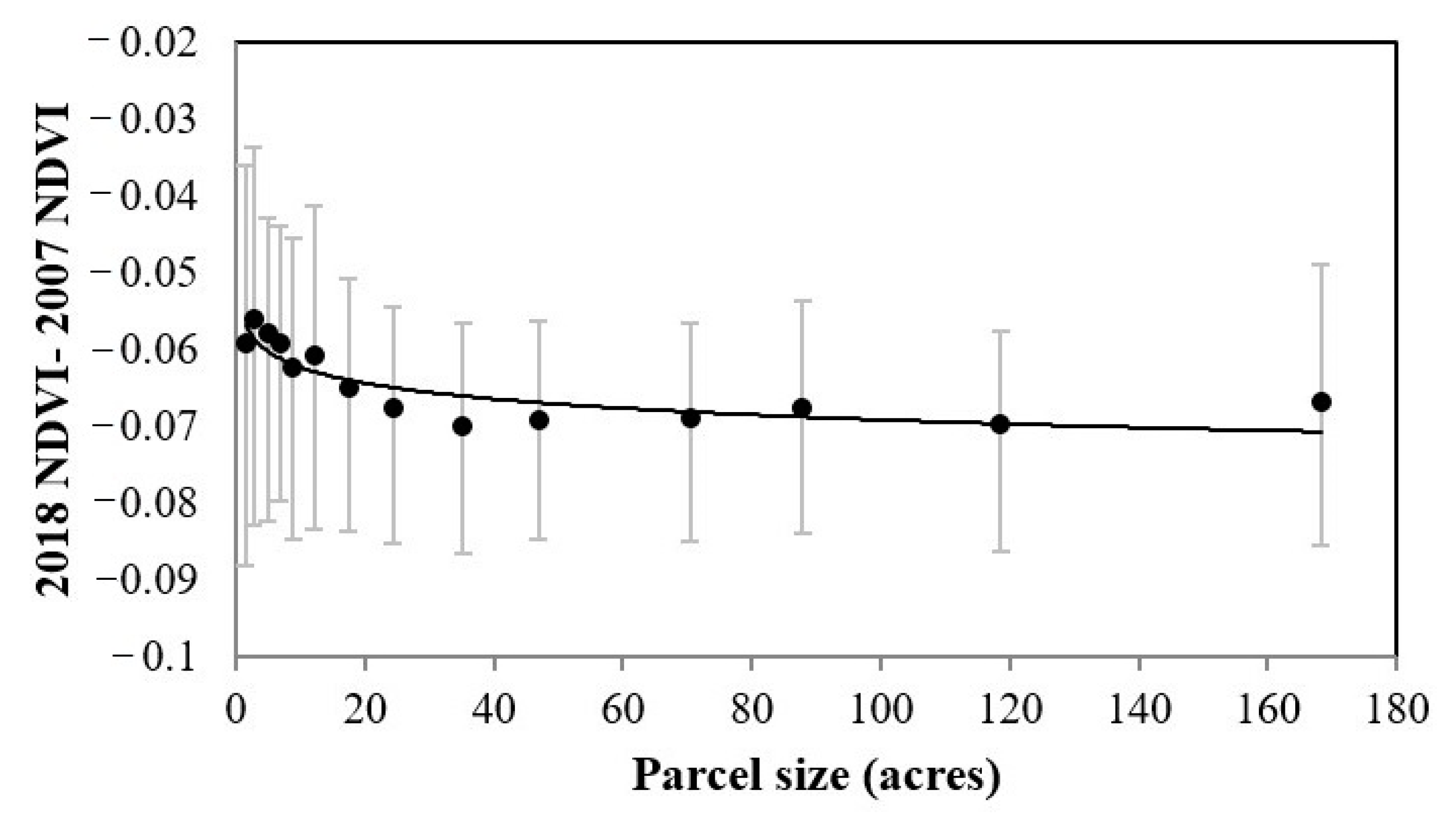
4.2.2. Forest Structural Attributes

Forest greenness represented by the NDVI values shows that greenness in both peak season and descending season has an increasing trend with parcel size (Figure 11). The variability of NDVI in peak season is smaller than that in the descending season in large parcels. The possible reason is that forests in large parcels are dense so that the NDVI values saturate in peak season. Nevertheless, the saturation problem is not serious in descending season so that forestlands with similar large parcel size have more significant difference in NDVI values. More importantly, the mean NDVI values in both peak season and descending season reach a stable value when parcel size is larger than 30 acres. Logarithmic model fitted the relationship of both peak-season NDVI and descending-season NDVI very well (R2 values are 0.93 and 0.89 respectively), and the peak-season NDVI changes faster with parcel size than descending-season NDVI (rate of change: 0.0074 vs. 0.0062).
Aboveground biomass also increases with parcel size (Figure 12). The mean AGB of bins increases from 80 tons/acre in small parcels to 110 tons/acre in large parcels. The mean AGB of bins also reaches a stable value around 110 tons/acre when parcels are larger than 30 acres. This non-linear relationship can be quantified by a logarithmic model (R2: 0.88). The large range of AGB in each bin indicates parcels with similar size have very different AGB values in the study area. AGB indicates the amount of carbon stored in vegetation. Figure 12 suggests that large parcels have higher ability to sequestrate carbon than small parcels.
LiDAR tree height and LiDAR intensity both show a clear pattern with parcel size (Figure 13). The average tree height increases from 37 feet in parcels of 1–2 acres to 47 feet in parcels of 30–40 acres and becomes stable after 30–40 acres. The leaf-off LiDAR intensity decreases with parcel size and also becomes stable when parcels are larger than 30 acres, suggesting that stem volume is higher in larger parcels. The relationship of both canopy height and leaf-off LiDAR intensity against parcel size can also be well modeled by the logarithmic regression (R2: 0.85).

5. Discussion

From Figure 9, Figure 10, Figure 11, Figure 12 and Figure 13, we can conclude that forests in small parcels may experience more disturbances than large parcels and consequently forests in small parcels are generally thinner, younger, shorter, and have lower abundance of oak trees. The good performance of logarithmic regression for modeling the relationship of various forest compositional and structural attributes suggests that forest composition and structure change rapidly with parcel size but this change slows down after a certain parcel size. Specifically, results of this study show that forests in parcels of 30 acre or larger are relatively stable. From the relevant literature and field investigation in our study area, the following possible reasons were explored.
First, forestland parcelization reduces forest coverage and increases forest fragmentation (i.e., the division of larger forest patches into disconnected small patches) and edge effects [37]. This is because the ownership transfers are often associated with liquidation cuts [7] or forestlands are developed by new owners for agriculture, logging, or settlement purposes [10,38]. A study in France using historical cadastral map and aerial photographs detected both fragmentation and a decrease in total forest area following the conversion of forest into agriculture during forestland parcelization process [39]. Gustafson and Loehle used a timber harvest simulator and neutral model landscapes to systematically study how parcelization affects forest fragmentation and found that parcelization of landscapes significantly increased forest fragmentation [12]. A previous study in Hocking County found that tourism grew dramatically because Hocking County has natural beauty and is close to the capital city of Ohio, Columbus. As a result, many smallholders built hot-tub cabins in forestlands to attract visitors [28].
Second, ownership parcelization may change forest composition and structure. Landowners often have different purposes from the previous owners for owing forestland and thus use different management practices [40]. As a result, the forest with different management practices may change the forest composition and structure compared to the mature old-growth forests [27]. A previous study based on interviews of smallholders in Southeastern Ohio found that smallholders implement different management practices for maximizing their own benefits [41]. In addition, forest fragmentation has undoubtedly negative effects on levels of pollination and seed production which may further change forest composition and structure [24].
Third, it has been demonstrated that forestland parcelization alters the original habitat conditions, connectivity and microenvironment [11,42]. When the native forests become more fragmented, the remnant forest patches are threatened as the remnant forests become more and more isolated. Matlack studied the microenvironmental gradients in Southeastern Pennsylvania and Northern Delaware and found significant edge effects in light, temperature, littler moisture, vapor pressure deficit and humidity [11]. These habitat changes and increased edge effects have negative effects on biodiversity and wildlife population, especially for the endangered species [2,43].
Fourth, it is difficult to implement sustainable forest management in small land parcels. From an ecological perspective, small forestland cannot be efficiently managed as a sustainable unit with most traditional ecological methods [5]. Belin et al. applied a mail-back survey method [44], which was proposed by Dillman [45], to obtain demographic information, gauge respondents’ attitudes toward the three indices of an ecosystem-based management approach, and measure landowner preferences toward issues surrounding forest conservation. Then, the authors used statistical tests to analyze the results and found that 26% of the respondents have a neutral attitude or agree that ecological health of their forest is not as important as their economic needs. Previous studies found that forestland parcelzation happens more often in private lands than public lands [37,46], and our study found that public forestland has healthier forests than private land (Table 2). Therefore, public purchases of small private forests which are adjacent to public land and under threat, could be a solution for forest conservation [46], or local government may open up a dialogue for more restrictive local land use polices for conserving forest [47].
This study has some limitations which can be further improved in the future. First, errors in the remote sensing derived products, especially the aboveground biomass, forest type map, may introduce uncertainties in the relationship between these forest attributes and the parcel size. This study applied the cutting-edge methods developed recently and specifically in the study area to estimate biomass and map forest types, as well as binning strategy to mitigate the impact of pixel-wise errors. However, to better know whether these errors affect the analysis of forest attributes in different parcel sizes, further study needs to collect more ground reference data to investigate the spatial distribution of errors. Compared with biomass and forest type, the products derived from LiDAR data are more accurate and reliable, such as the tree height and LiDAR intensity. Second, we did not study the trajectory of land parcelization because such ownership transition data in our study area is not available. In this study, we used forests in different parcel sizes to represent different stages of parcelization. Considering that the other environmental conditions in the study area are relatively homogenous, differences in forest attributes among parcels should be able to imply the influence of forest parcelization. If the trajectory of forestland ownership is available, it is worth exploring the short-term and long-term forest changes after the ownership deviation. Third, we did not apply multi-year remotely sensed data to monitor the forest attribute change because of the limitation of training samples for mapping forest attributes in other years. Alternatively, we compared autumn NDVI derived from two Landsat images (Landsat-5 TM image on Sep. 24, 2007 and Landsat-8 OLI image on Oct. 8, 2018) to obtain some preliminary results. The result shows that NDVI changes (i.e., 2018 NDVI - 2007 NDVI) of both public and private lands are marginal (-0.07 vs. -0.06) and this minor NDVI decrease is mainly due to the 14-day seasonal difference between two images, suggesting that both private and public forests did not experience large change in the 12-year period. It is interesting that small parcels have a slightly smaller NDVI decrease than large parcels (Figure 14). A possible reason is that young trees in small parcels have rapid canopy development during the 12-year period while mature trees in large parcels are more stable. The impact of land parcelization is a long-term process, so long-term satellite images are needed by future studies to explore the temporal change of forests with different sizes. Forth, forest composition and structure may be affected by other environmental factors besides land parcelization, such as elevation. Our study area does not have large elevation variation (mean elevation 283 m, and standard deviation 31 m) and there is no significant elevation trend with parcel size, but elevation variation may introduce uncertainty in the findings of this study. Future studies should take more factors into account when exploring the impact of land parcelization on forest development.

6. Conclusions

This study used multi-source remotely sensed data to investigate the impact of parcel size on forest composition and structure in the Southeastern Ohio. There are some interesting findings: (1) larger parcels have a larger proportion of forest cover; (2) for small parcels, such as parcels between 1 and 10 acres, a large portion of land is used for construction and farming; (3) there is an increasing trend of NDVI with parcel size, but it saturates when parcels are larger than 30 acres; (4) trees are higher in larger parcels than small parcels; and (5) these nonlinear relationships between forest attributes and parcel size can be quantified by logarithmic regression models. These findings are consistent with existing studies, i.e., forests in smaller parcels may have more disturbances than in larger parcels because of the frequent land transactions and management practices, and forests in small parcels make it difficult to implement sustainable management. As a result, forests in larger parcels are generally denser, higher and more mature than those in smaller parcels.
Another implication of this study is that it demonstrates a successful example of using remote sensing data to investigate the impact of forest ownership. It is a valuable supplement to the traditional field surveying and interview of land holders. It could be applied to study larger area if both ownership and remote sensing data are available. Studies with more sites could help to achieve a comprehensive understanding of the impact of land parcelization on forest composition and structure.

Author Contributions

Conceptualization, X.Z. and D.L.; methodology, X.Z. and D.L.; formal analysis, X.Z.; investigation, X.Z.; resources, X.Z. and D.L.; writing, X.Z. and D.L.; funding acquisition, X.Z. and D.L.

Funding

This research was funded by the Research Grants Council of Hong Kong, grant number 25222717, Research Institute for Sustainable Urban Development, the Hong Kong Polytechnic University, grant number 1-BBWD, and the National Science Foundation of the USA, grant number 1010314.

Conflicts of Interest

The authors declare no conflict of interest.

References

  1. Gong, P.; Wang, J.; Yu, L.; Zhao, Y.; Zhao, Y.; Liang, L.; Niu, Z.; Huang, X.; Fu, H.; Liu, S.; et al. Finer resolution observation and monitoring of global land cover: First mapping results with Landsat TM and ETM+ data. Int. J. Remote Sens. 2013, 34, 2607–2654. [Google Scholar] [CrossRef]
  2. Butler, B.J.; Hewes, J.H.; Dickinson, B.J.; Andrejczyk, K.; Butler, S.M.; Markowski-Lindsay, M. Family Forest Ownerships of the United States, 2013: Findings from the USDA Forest Service’s National Woodland Owner Survey. J. For. 2016, 114, 638–647. [Google Scholar] [CrossRef]
  3. Boring, L.R.; Monk, C.D.; Swank, W.T. Early regeneration of a clear-cut southern Appalachian forest. Ecology 1981, 62, 1244–1253. [Google Scholar] [CrossRef]
  4. Kilgore, M.A.; Snyder, S.A. Exploring the relationship between parcelization metrics and natural resource managers’ perceptions of forest land parcelization intensity. Landsc. Urban Plan. 2016. [Google Scholar] [CrossRef]
  5. Sampson, N.; DeCoster, L. Forest fragmentation: Implications for sustainable private forests. J. For. 2000, 98, 4–8. [Google Scholar] [CrossRef]
  6. Mehmood, S.; Zhang, D. Forest parcelization in the United States: A study of contributing factors. J. For. 2001, 99, 30–34. [Google Scholar]
  7. Germain, R.H.; Anderson, N.; Bevilacqua, E. The effects of forestland parcelization and ownership transfers on nonindustrial private forestland forest stocking in New York. J. For. 2007, 105, 403–408. [Google Scholar]
  8. Ko, D.W.; He, H.S.; Larsen, D.R. Simulating private land ownership fragmentation in the Missouri Ozarks, USA. Landsc. Ecol. 2006, 21, 671–686. [Google Scholar] [CrossRef]
  9. Donnelly, S.; Evans, T.P. Characterizing spatial patterns of land ownership at the parcel level in south-central Indiana, 1928–1997. Landsc. Urban Plan. 2008, 84, 230–240. [Google Scholar] [CrossRef]
  10. Haines, A.L.; Kennedy, T.T.; McFarlane, D.L. Parcelization: Forest change agent in Northern Wisconsin. J. For. 2011, 109, 101–108. [Google Scholar]
  11. Matlack, G.R. Microenvironment variation within and among forest edge sites in the eastern United States. Biol. Conserv. 1993, 66, 185–194. [Google Scholar] [CrossRef]
  12. Gustafson, E.J.; Loehle, C. Effects of parcelization and land divestiture on forest sustainability in simulated forest landscapes. For. Ecol. Manag. 2006, 236, 305–314. [Google Scholar] [CrossRef]
  13. Frayer, W.E.; Furnival, G.M. Forest survey sampling designs—A history. J. For. 1999, 97, 4–10. [Google Scholar] [CrossRef]
  14. Gardner, T.A.; Barlow, J.; Araujo, I.S.; Ávila-Pires, T.C.; Bonaldo, A.B.; Costa, J.E.; Esposito, M.C.; Ferreira, L.V.; Hawes, J.; Hernandez, M.I.M.; et al. The cost-effectiveness of biodiversity surveys in tropical forests. Ecol. Lett. 2008, 11, 139–150. [Google Scholar] [CrossRef]
  15. McRoberts, R.E.; Tomppo, E.O. Remote sensing support for national forest inventories. Remote Sens. Environ. 2007, 110, 412–419. [Google Scholar] [CrossRef]
  16. Wulder, M. Optical remote-sensing techniques for the assessment of forest inventory and biophysical parameters. Prog. Phys. Geogr. 1998, 22, 449–476. [Google Scholar] [CrossRef]
  17. Sexton, J.O.; Song, X.P.; Feng, M.; Noojipady, P.; Anand, A.; Huang, C.; Kim, D.H.; Collins, K.M.; Channan, S.; DiMiceli, C.; et al. Global, 30-m resolution continuous fields of tree cover: Landsat-based rescaling of MODIS vegetation continuous fields with lidar-based estimates of error. Int. J. Digit. Earth 2013, 6, 427–448. [Google Scholar] [CrossRef] [Green Version]
  18. Hogland, J.; Anderson, N.; Affleck, D.L.R.; St. Peter, J. Using Forest Inventory Data with Landsat 8 Imagery to Map Longleaf Pine Forest Characteristics in Georgia, USA. Remote Sens. 2019, 11, 1803. [Google Scholar] [CrossRef]
  19. Rahman, M.T.; Rashed, T. Urban tree damage estimation using airborne laser scanner data and geographic information systems: An example from 2007 Oklahoma ice storm. Urban For. Urban Green. 2015, 14, 562–572. [Google Scholar] [CrossRef]
  20. Brilli, L.; Chiesi, M.; Brogi, C.; Magno, R.; Arcidiaco, L.; Bottai, L.; Tagliaferri, G.; Bindi, M.; Maselli, F. Combination of ground and remote sensing data to assess carbon stock changes in the main urban park of Florence. Urban For. Urban Green. 2019, 43, 126377. [Google Scholar] [CrossRef]
  21. Tortini, R.; Mayer, A.L.; Hermosilla, T.; Coops, N.C.; Wulder, M.A. Using annual Landsat imagery to identify harvesting over a range of intensities for non-industrial family forests. Landsc. Urban Plan. 2019, 188, 143–150. [Google Scholar] [CrossRef]
  22. Midha, N.; Mathur, P.K. Assessment of forest fragmentation in the conservation priority Dudhwa landscape, India using FRAGSTATS computed class level metrics. J. Indian Soc. Remote Sens. 2010, 38, 487–500. [Google Scholar] [CrossRef]
  23. Croissant, C. Landscape patterns and parcel boundaries: An analysis of composition and configuration of land use and land cover in south-central Indiana. Agric. Ecosyst. Environ. 2004, 101, 219–232. [Google Scholar] [CrossRef]
  24. Aizen, M.A.; Feinsinger, P. Forest fragmentation, pollination, and plant reproduction in a chaco dry forest, Argentina. Ecology 1994, 75, 330–351. [Google Scholar] [CrossRef]
  25. Virgós, E.; Tellería, J.L.; Santos, T. A comparison on the response to forest fragmentation by medium-sized Iberian carnivores in central Spain. Biodivers. Conserv. 2002, 11, 1063–1079. [Google Scholar] [CrossRef]
  26. Gordon, R.B. The Natural Vegetation of Ohio in Pioneer Days; Ohio State University: Columbus, OH, USA, 1969. [Google Scholar]
  27. Drury, S.A.; Runkle, J.R. Forest vegetation change in southeast Ohio: Do older forests serve as useful models for predicting the successional trajectory of future forests? For. Ecol. Manag. 2006, 223, 200–210. [Google Scholar] [CrossRef]
  28. Van Berkel, D.B.; Munroe, D.K.; Gallemore, C. Spatial analysis of land suitability, hot-tub cabins and forest tourism in Appalachian Ohio. Appl. Geogr. 2014, 54, 139–148. [Google Scholar] [CrossRef]
  29. Nassauer, J.I.; Cooper, D.A.; Marshall, L.L.; Currie, W.S.; Hutchins, M.; Brown, D.G. Parcel size related to household behaviors affecting carbon storage in exurban residential landscapes. Landsc. Urban Plan. 2014, 129, 55–64. [Google Scholar] [CrossRef]
  30. Zhu, X.; Liu, D. Improving forest aboveground biomass estimation using seasonal Landsat NDVI time-series. ISPRS J. Photogramm. Remote Sens. 2015, 102, 222–231. [Google Scholar] [CrossRef]
  31. Zhu, X.; Liu, D. Accurate mapping of forest types using dense seasonal landsat time-series. ISPRS J. Photogramm. Remote Sens. 2014, 96, 1–11. [Google Scholar] [CrossRef]
  32. Riaño, D.; Chuvieco, E.; Salas, J.; Aguado, I. Assessment of different topographic corrections in landsat-TM data for mapping vegetation types (2003). IEEE Trans. Geosci. Remote Sens. 2003. [Google Scholar] [CrossRef]
  33. Kim, S.; McGaughey, R.J.; Andersen, H.E.; Schreuder, G. Tree species differentiation using intensity data derived from leaf-on and leaf-off airborne laser scanner data. Remote Sens. Environ. 2009, 113, 1575–1586. [Google Scholar] [CrossRef]
  34. Fei, S.; Kong, N.; Steiner, K.C.; Moser, W.K.; Steiner, E.B. Change in oak abundance in the eastern United States from 1980 to 2008. For. Ecol. Manag. 2011, 262, 1370–1377. [Google Scholar] [CrossRef]
  35. Gu, Y.; Wylie, B.K.; Howard, D.M.; Phuyal, K.P.; Ji, L. NDVI saturation adjustment: A new approach for improving cropland performance estimates in the Greater Platte River Basin, USA. Ecol. Indic. 2013, 30, 1–6. [Google Scholar] [CrossRef]
  36. An, S.; Zhu, X.; Shen, M.; Wang, Y.; Cao, R.; Chen, X.; Yang, W.; Chen, J.; Tang, Y. Mismatch in elevational shifts between satellite observed vegetation greenness and temperature isolines during 2000–2016 on the Tibetan Plateau. Glob. Chang. Biol. 2018, 24, 5411–5425. [Google Scholar] [CrossRef] [PubMed]
  37. Mayer, A.L. Family forest owners and landscape-scale interactions: A review. Landsc. Urban Plan. 2019, 188, 4–18. [Google Scholar] [CrossRef]
  38. Mundell, J.; Taff, S.J.; Kilgore, M.A.; Snyder, S.A. Using real estate records to assess forest land parcelization and development: A Minnesota case study. Landsc. Urban Plan. 2010, 94, 71–76. [Google Scholar] [CrossRef]
  39. Andrieu, E.; Ladet, S.; Heintz, W.; Deconchat, M. History and spatial complexity of deforestation and logging in small private forests. Landsc. Urban Plan. 2011, 103, 109–117. [Google Scholar] [CrossRef]
  40. Floress, K.; Huff, E.S.; Snyder, S.A.; Koshollek, A.; Butler, S.; Allred, S.B. Factors associated with family forest owner actions: A vote-count meta-analysis. Landsc. Urban Plan. 2019, 188, 19–29. [Google Scholar] [CrossRef]
  41. Law, J.; McSweeney, K. Looking under the canopy: Rural smallholders and forest recovery in Appalachian Ohio. Geoforum 2013, 44, 182–192. [Google Scholar] [CrossRef]
  42. Heilman, G.E., Jr.; Strittholt, J.R.; Slosser, N.C.; Dellasala, D.A. Forest fragmentation of the conterminous United States: Assessing forest intactness through road density and spatial characteristics. Bioscience 2002, 52, 411–422. [Google Scholar] [CrossRef]
  43. Bagarinao, R.T. Forest fragmentation in Central Cebu and its potential causes: A landscape ecological approach. J. Environ. Sci. Manag. 2010, 34, 487–515. [Google Scholar] [CrossRef]
  44. Belin, D.L.; Kittredge, D.B.; Stevens, T.H.; Dennis, D.C.; Schweik, C.M.; Morzuch, B.J. Assessing private forest owner attitudes toward ecosystem-based management. J. For. 2005, 103, 28–35. [Google Scholar]
  45. Dillman, D.A. Mail and Internet Surveys: The Tailored Design Method, 2nd ed.; John Wiley & Sons Inc.: Hoboken, NJ, USA, 2007; ISBN 0-7803-1482-4. [Google Scholar]
  46. L’Roe, A.W.; Rissman, A.R. Factors that influence working forest conservation and parcelization. Landsc. Urban Plan. 2017, 167, 14–24. [Google Scholar] [CrossRef]
  47. Haines, A.L.; Thompson, A.W.; McFarlane, D.; Sharp, A.K. Local policy and landowner attitudes: A case study of forest fragmentation. Landsc. Urban Plan. 2019, 188, 97–109. [Google Scholar] [CrossRef]
Figure 1. The study area (Hocking County in Southeastern Ohio, USA) and the parcels of land ownership.
Remotesensing 11 02195 g001
Figure 2. Flowchart of using Landsat imagery and LiDAR data to investigate the impact of land parcelization on forest development.
Remotesensing 11 02195 g002
Figure 3. Forest types map derived from Landsat time series.
Remotesensing 11 02195 g003
Figure 4. Normalized difference vegetation index (NDVI) values of Landsat image acquired in the peak season (20 June).
Remotesensing 11 02195 g004
Figure 5. Above ground biomass estimated from seasonal NDVI time-series by an artificial neural network model.
Remotesensing 11 02195 g005
Figure 6. Canopy height estimated from LiDAR data.
Remotesensing 11 02195 g006
Figure 7. A subset of true color of leaf-on Landsat image on June 20 (a) and its corresponding leaf-off LiDAR intensity; (b): lower LiDAR intensity is related to Landsat pixels with high forest density (dark green color).
Remotesensing 11 02195 g007
Figure 8. Private parcels were divided into 14 bins for exploring the relationship between forest attributes and parcel size. A bin of a-b acres includes all parcels of a≤ parcel size <b.
Remotesensing 11 02195 g008
Figure 9. Percentage of forest versus parcel size (a) and percentage of non-vegetation (e.g., urban, bare land, and water) versus parcel size; (b). The black point is mean value of each bin, the error bar is the 0.25-0.75 percentiles, and the solid line is the regression line.
Remotesensing 11 02195 g009
Figure 10. Abundance of oak trees versus parcel size. The black point is the mean value of each bin, the error bar is the 0.25–0.75 percentiles, and the solid line is the regression line.
Remotesensing 11 02195 g010
Figure 11. NDVI values in peak season versus parcel size (a) and NDVI values in descending season versus parcel size; (b). The black point is mean value of each bin, the error bar is the 0.25–0.75 percentiles, and the solid line is the regression line.
Remotesensing 11 02195 g011
Figure 12. Aboveground biomass (AGB) values versus parcel size. The black point is mean value of each bin, the error bar is the 0.25–0.75 percentiles, and the solid line is the regression line.
Remotesensing 11 02195 g012
Figure 13. LiDAR Canopy height versus parcel size (a) and LiDAR intensity versus parcel size; (b). The black point is mean value of each bin, the error bar is the 0.25–0.75 percentiles, and the solid line is the regression line.
Remotesensing 11 02195 g013
Figure 14. Autumn NDVI change between 2018 and 2007 versus parcel sizes. The black point is mean value of each bin, the error bar is the 0.25–0.75 percentiles, and the solid line is the regression line.
Remotesensing 11 02195 g014
Table 1. Summary of parcel size of private and public lands larger than 1 acre in Hocking County, Ohio (unit: acre).
OwnershipNumber of ParcelsMinimumMaximum MeanMedianStandard Deviation
Private lands101651975.921.5643.4
Public lands1361.61503.6275244.4242.3
Table 2. Comparison of forest attributes between private and public lands by t-test (sd = standard deviation; Ha = alternative hypothesis).
Forest AttributesPrivate LandsPublic LandsHat-Testp-Value
mean1sd1mean2sd2
Forest coverage64.02235.08290.02021.201mean2>mean114.046<0.0001
Peak NDVI0.7790.0310.7970.016mean2>mean112.704<0.0001
Fall NDVI0.6480.0390.6660.026mean2>mean18.214<0.0001
Lidar tree height41.94312.45150.63810.907mean2>mean19.217<0.0001
Lidar intensity114.40229.67783.60624.331mean2<mean114.619<0.0001
AGB92.77635.379113.89128.384mean2>mean18.451<0.0001

