Conditional Generative Adversarial Networks (cGANs) for Near Real-Time Precipitation Estimation from Multispectral GOES-16 Satellite Imageries—PERSIANN-cGAN

 , ,
, ,  ,
, 
Abstract
1. Introduction
2. Materials and Study Region
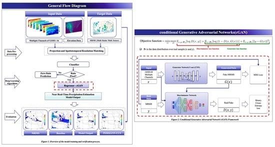
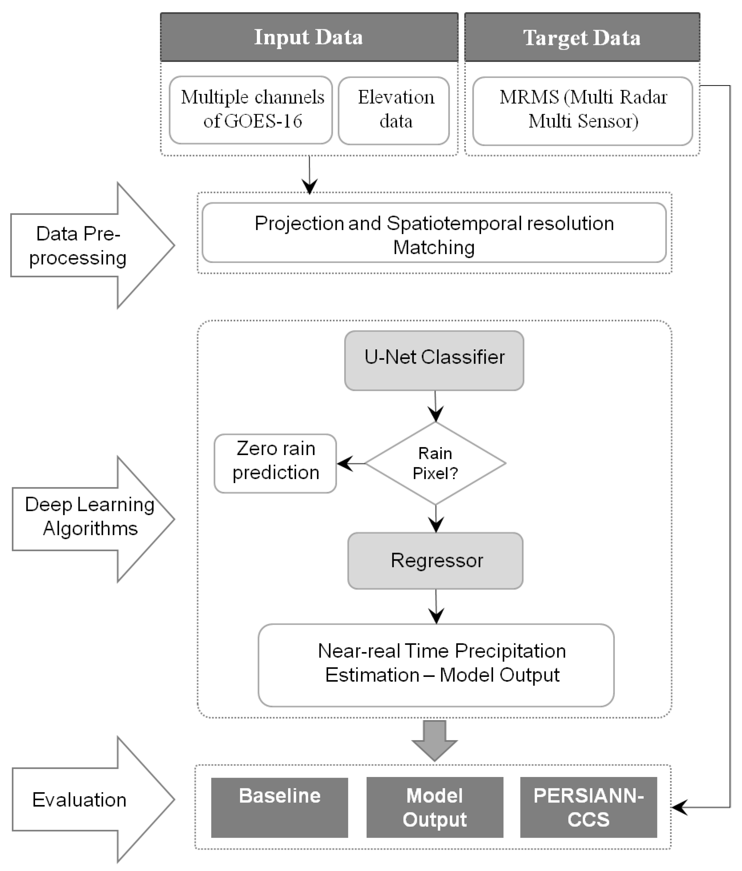
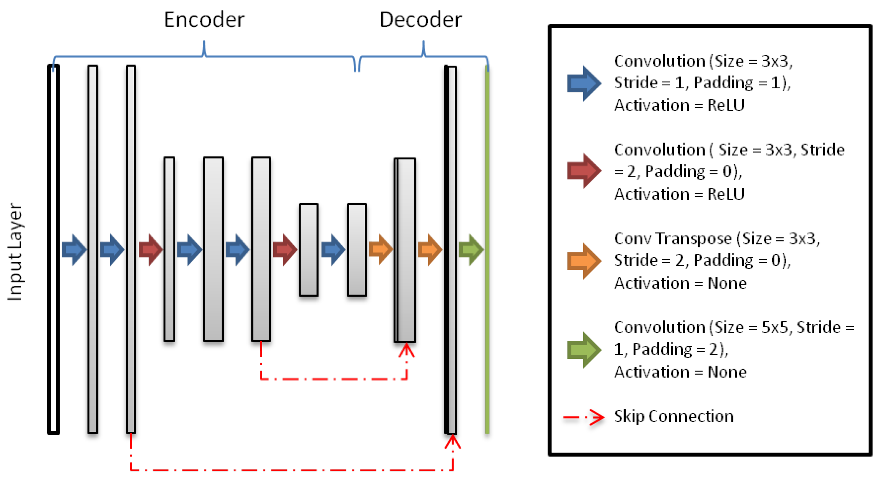
3. Methodology
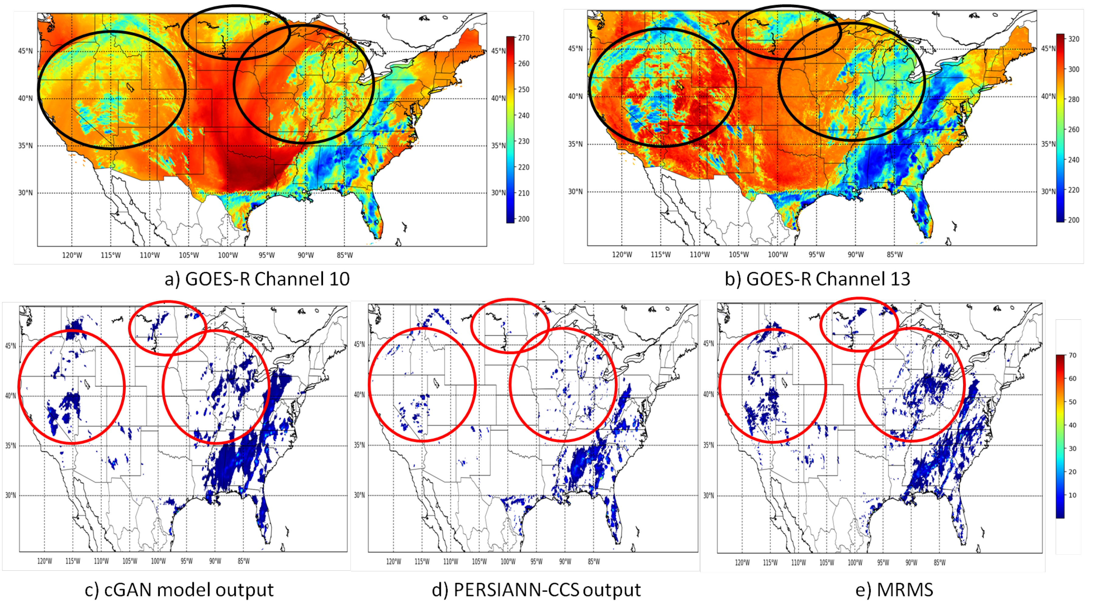
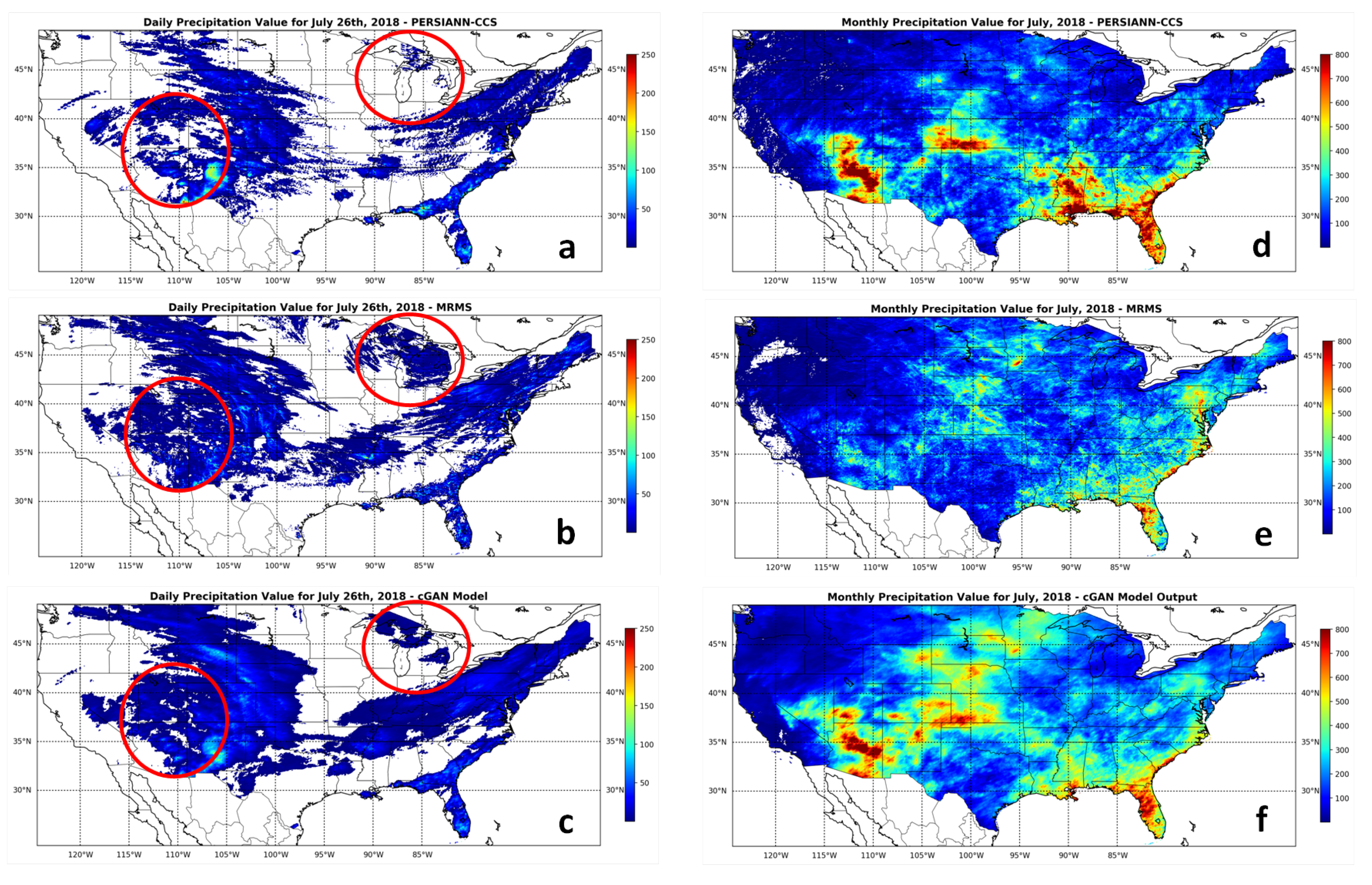
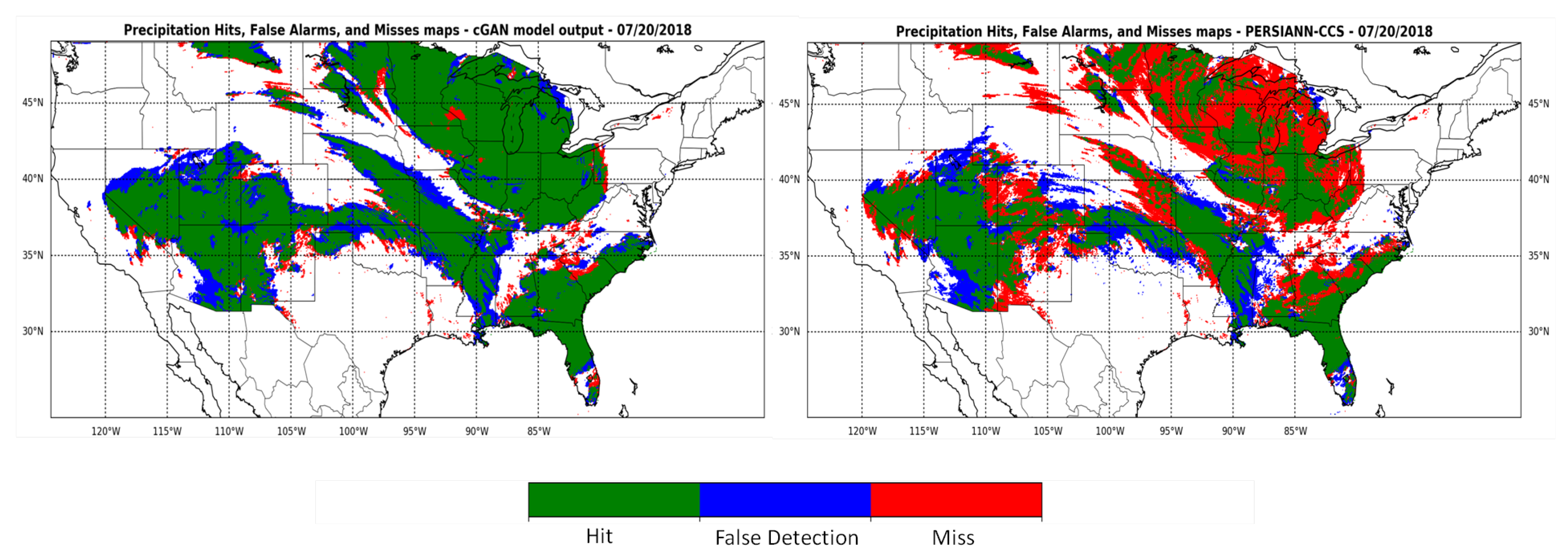
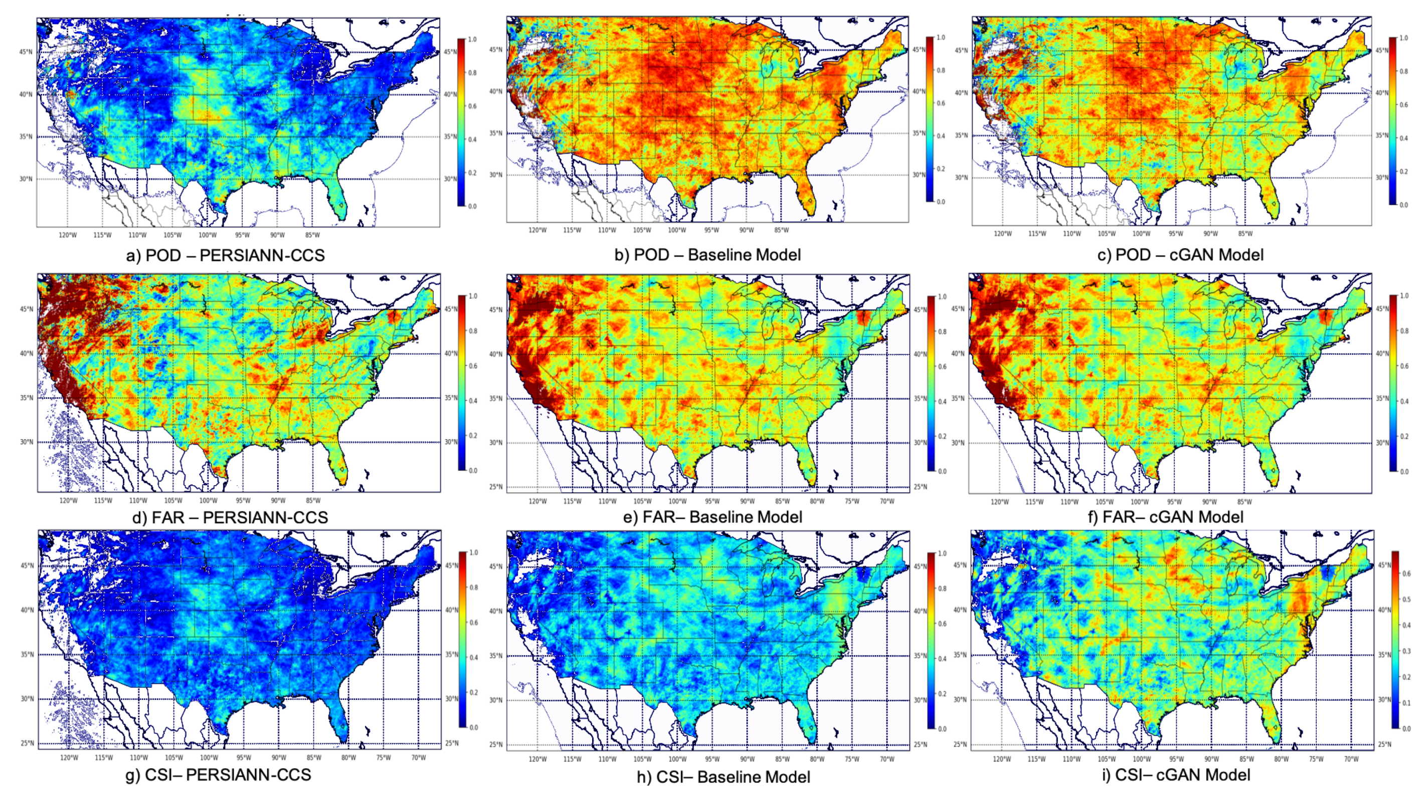
4. Results
5. Conclusions
Author Contributions
Funding
Acknowledgments
Conflicts of Interest
References
- Sorooshian, S.; AghaKouchak, A.; Arkin, P.; Eylander, J.; Foufoula-Georgiou, E.; Harmon, R.; Hendrickx, J.M.; Imam, B.; Kuligowski, R.; Skahill, B.; et al. Advanced concepts on remote sensing of precipitation at multiple scales. Bull. Am. Meteorol. Soc. 2011, 92, 1353–1357. [Google Scholar] [CrossRef]
- Nguyen, P.; Shearer, E.J.; Tran, H.; Ombadi, M.; Hayatbini, N.; Palacios, T.; Huynh, P.; Braithwaite, D.; Updegraff, G.; Hsu, K.; et al. The CHRS Data Portal, an easily accessible public repository for PERSIANN global satellite precipitation data. Sci. Data 2019, 6, 180296. [Google Scholar] [CrossRef] [PubMed]
- Ba, M.B.; Gruber, A. GOES multispectral rainfall algorithm (GMSRA). J. Appl. Meteorol. 2001, 40, 1500–1514. [Google Scholar] [CrossRef]
- Behrangi, A.; Imam, B.; Hsu, K.; Sorooshian, S.; Bellerby, T.J.; Huffman, G.J. REFAME: Rain estimation using forward-adjusted advection of microwave estimates. J. Hydrometeorol. 2010, 11, 1305–1321. [Google Scholar] [CrossRef]
- Behrangi, A.; Hsu, K.l.; Imam, B.; Sorooshian, S.; Huffman, G.J.; Kuligowski, R.J. PERSIANN-MSA: A precipitation estimation method from satellite-based multispectral analysis. J. Hydrometeorol. 2009, 10, 1414–1429. [Google Scholar] [CrossRef]
- Behrangi, A.; Hsu, K.l.; Imam, B.; Sorooshian, S.; Kuligowski, R.J. Evaluating the utility of multispectral information in delineating the areal extent of precipitation. J. Hydrometeorol. 2009, 10, 684–700. [Google Scholar] [CrossRef]
- Martin, D.W.; Kohrs, R.A.; Mosher, F.R.; Medaglia, C.M.; Adamo, C. Over-ocean validation of the global convective diagnostic. J. Appl. Meteorol. Climatol. 2008, 47, 525–543. [Google Scholar] [CrossRef]
- Tao, Y.; Gao, X.; Ihler, A.; Hsu, K.; Sorooshian, S. Deep neural networks for precipitation estimation from remotely sensed information. In Proceedings of the 2016 IEEE Congress on Evolutionary Computation (CEC), Vancouver, BC, Canada, 24–29 July 2016; pp. 1349–1355. [Google Scholar]
- Hayatbini, N.; Hsu, K.L.; Sorooshian, S.; Zhang, Y.; Zhang, F. Effective Cloud Detection and Segmentation Using a Gradient-Based Algorithm for Satellite Imagery: Application to Improve PERSIANN-CCS. J. Hydrometeorol. 2019, 20, 901–913. [Google Scholar] [CrossRef]
- Joyce, R.J.; Janowiak, J.E.; Arkin, P.A.; Xie, P. CMORPH: A method that produces global precipitation estimates from passive microwave and infrared data at high spatial and temporal resolution. J. Hydrometeorol. 2004, 5, 487–503. [Google Scholar] [CrossRef]
- Kidd, C.; Kniveton, D.R.; Todd, M.C.; Bellerby, T.J. Satellite rainfall estimation using combined passive microwave and infrared algorithms. J. Hydrometeorol. 2003, 4, 1088–1104. [Google Scholar] [CrossRef]
- Huffman, G.J.; Bolvin, D.T.; Braithwaite, D.; Hsu, K.; Joyce, R.; Xie, P.; Yoo, S.H. NASA global precipitation measurement (GPM) integrated multi-satellite retrievals for GPM (IMERG). Algorithm Theor. Basis Doc. Version 2015, 4, 30. [Google Scholar]
- Huffman, G.J.; Bolvin, D.T.; Nelkin, E.J.; Wolff, D.B.; Adler, R.F.; Gu, G.; Hong, Y.; Bowman, K.P.; Stocker, E.F. The TRMM multisatellite precipitation analysis (TMPA): Quasi-global, multiyear, combined-sensor precipitation estimates at fine scales. J. Hydrometeorol. 2007, 8, 38–55. [Google Scholar] [CrossRef]
- Hong, Y.; Hsu, K.L.; Sorooshian, S.; Gao, X. Precipitation estimation from remotely sensed imagery using an artificial neural network cloud classification system. J. Appl. Meteorol. 2004, 43, 1834–1853. [Google Scholar] [CrossRef]
- Tao, Y.; Hsu, K.; Ihler, A.; Gao, X.; Sorooshian, S. A two-stage deep neural network framework for precipitation estimation from Bispectral satellite information. J. Hydrometeorol. 2018, 19, 393–408. [Google Scholar] [CrossRef]
- Bengio, Y. Learning deep architectures for AI. Found. Trends Mach. Learn. 2009, 2, 1–127. [Google Scholar] [CrossRef]
- Hinton, G.E. Deep belief networks. Scholarpedia 2009, 4, 5947. [Google Scholar] [CrossRef]
- LeCun, Y.; Bengio, Y.; Hinton, G. Deep learning. Nature 2015, 521, 436. [Google Scholar] [CrossRef] [PubMed]
- Liu, Z.; Zhou, P.; Chen, X.; Guan, Y. A multivariate conditional model for streamflow prediction and spatial precipitation refinement. J. Geophys. Res. Atmos. 2015, 120. [Google Scholar] [CrossRef]
- Rasp, S.; Pritchard, M.S.; Gentine, P. Deep learning to represent subgrid processes in climate models. Proc. Natl. Acad. Sci. USA 2018, 115, 9684–9689. [Google Scholar] [CrossRef]
- Reichstein, M.; Camps-Valls, G.; Stevens, B.; Jung, M.; Denzler, J.; Carvalhais, N.; Prabhat. Deep learning and process understanding for data-driven Earth system science. Nature 2019, 566, 195. [Google Scholar] [CrossRef]
- Akbari Asanjan, A.; Yang, T.; Hsu, K.; Sorooshian, S.; Lin, J.; Peng, Q. Short-Term Precipitation Forecast Based on the PERSIANN System and LSTM Recurrent Neural Networks. J. Geophys. Res. Atmos. 2018, 123, 12–543. [Google Scholar] [CrossRef]
- Pan, B.; Hsu, K.; AghaKouchak, A.; Sorooshian, S. Improving Precipitation Estimation Using Convolutional Neural Network. Water Resour. Res. 2019, 55, 2301–2321. [Google Scholar] [CrossRef]
- Goodfellow, I.; Bengio, Y.; Courville, A. Deep Learning; MIT Press: Cambridge, MA, USA, 2016; Available online: http://www.deeplearningbook.org (accessed on 20 September 2019).
- Schmidhuber, J. Deep learning in neural networks: An overview. Neural Netw. 2015, 61, 85–117. [Google Scholar] [CrossRef] [PubMed]
- Shen, D.; Wu, G.; Suk, H.I. Deep learning in medical image analysis. Annu. Rev. Biomed. Eng. 2017, 19, 221–248. [Google Scholar] [CrossRef] [PubMed]
- Vandal, T.; Kodra, E.; Ganguly, A.R. Intercomparison of machine learning methods for statistical downscaling: The case of daily and extreme precipitation. Theor. Appl. Climatol. 2019, 137, 557–570. [Google Scholar] [CrossRef]
- Tao, Y.; Gao, X.; Ihler, A.; Sorooshian, S.; Hsu, K. Precipitation identification with bispectral satellite information using deep learning approaches. J. Hydrometeorol. 2017, 18, 1271–1283. [Google Scholar] [CrossRef]
- Liu, Y.; Racah, E.; Prabhat; Correa, J.; Khosrowshahi, A.; Lavers, D.; Kunkel, K.; Wehner, M.; Collins, W. Application of deep convolutional neural networks for detecting extreme weather in climate datasets. arXiv 2016, arXiv:1605.01156. [Google Scholar]
- Xingjian, S.; Chen, Z.; Wang, H.; Yeung, D.Y.; Wong, W.K.; Woo, W.C. Convolutional LSTM network: A machine learning approach for precipitation nowcasting. In Advances in Neural Information Processing Systems; The MIT Press: Cambridge, MA, USA, 2015; pp. 802–810. [Google Scholar]
- LeCun, Y.; Boser, B.; Denker, J.S.; Henderson, D.; Howard, R.E.; Hubbard, W.; Jackel, L.D. Backpropagation applied to handwritten zip code recognition. Neural Comput. 1989, 1, 541–551. [Google Scholar] [CrossRef]
- Elman, J.L. Finding structure in time. Cogn. Sci. 1990, 14, 179–211. [Google Scholar] [CrossRef]
- Jordan, M.I. Serial order: A parallel distributed processing approach. In Advances in Psychology; Elsevier: Amsterdam, The Netherlands, 1997; Volume 121, pp. 471–495. [Google Scholar]
- Krizhevsky, A.; Sutskever, I.; Hinton, G.E. Imagenet classification with deep convolutional neural networks. In Advances in Neural Information Processing Systems; The MIT Press: Cambridge, MA, USA, 2012; pp. 1097–1105. [Google Scholar]
- Vincent, P.; Larochelle, H.; Bengio, Y.; Manzagol, P.A. Extracting and composing robust features with denoising autoencoders. In Proceedings of the 25th International Conference on Machine Learning, Helsinki, Finland, 5–9 July 2008; ACM: New York, NY, USA, 2008; pp. 1096–1103. [Google Scholar]
- Pu, Y.; Gan, Z.; Henao, R.; Yuan, X.; Li, C.; Stevens, A.; Carin, L. Variational autoencoder for deep learning of images, labels and captions. In Advances in Neural Information Processing Systems; The MIT Press: Cambridge, MA, USA, 2016; pp. 2352–2360. [Google Scholar]
- Goodfellow, I.; Pouget-Abadie, J.; Mirza, M.; Xu, B.; Warde-Farley, D.; Ozair, S.; Courville, A.; Bengio, Y. Generative adversarial nets. Advances in Neural Information Processing Systems; The MIT Press: Cambridge, MA, USA, 2014; pp. 2672–2680. [Google Scholar]
- Schmit, T.J.; Gunshor, M.M.; Menzel, W.P.; Gurka, J.J.; Li, J.; Bachmeier, A.S. Introducing the next-generation Advanced Baseline Imager on GOES-R. Bull. Am. Meteorol. Soc. 2005, 86, 1079–1096. [Google Scholar] [CrossRef]
- NOAA’s Comprehensive Large Array-data Stewardship System. Available online: https://www.avl.class.noaa.gov/saa/products/welcome/ (accessed on 1 October 2018).
- Schmit, T.J.; Menzel, W.P.; Gurka, J.; Gunshor, M. The ABI on GOES-R. In Proceedings of the 6th Annual Symposium on Future National Operational Environmental Satellite Systems-NPOESS and GOES-R, Atlanta, GA, USA, 16–21 January 2010. [Google Scholar]
- GPM Ground Validation Data Archieve. Available online: https://gpm-gv.gsfc.nasa.gov/ (accessed on 1 November 2018).
- Danielson, J.J.; Gesch, D.B. Global Multi-Resolution Terrain Elevation Data 2010 (GMTED2010), Technical report; US Geological Survey: Reston, VA, USA, 2011. [Google Scholar]
- Ronneberger, O.; Fischer, P.; Brox, T. U-net: Convolutional networks for biomedical image segmentation. In Proceedings of the International Conference on Medical Image Computing and Computer-Assisted Intervention, Munich, Germany, 5–9 October 2015; Springer: Berlin, Germany, 2015; pp. 234–241. [Google Scholar]
- Arjovsky, M.; Chintala, S.; Bottou, L. Wasserstein gan. arXiv 2017, arXiv:1701.07875. [Google Scholar]
- Huszár, F. How (not) to train your generative model: Scheduled sampling, likelihood, adversary? arXiv 2015, arXiv:1511.05101. [Google Scholar]
- Goodfellow, I. NIPS 2016 tutorial: Generative adversarial networks. arXiv 2016, arXiv:1701.00160. [Google Scholar]
- Mirza, M.; Osindero, S. Conditional generative adversarial nets. arXiv 2014, arXiv:1411.1784. [Google Scholar]
- Isola, P.; Zhu, J.Y.; Zhou, T.; Efros, A.A. Image-to-image translation with conditional adversarial networks. In Proceedings of the IEEE Conference on Computer Vision and Pattern Recognition, Honolulu, HI, USA, 21–26 July 2017; pp. 1125–1134. [Google Scholar]


| Band Number-Wavelength () | ||
|---|---|---|
| 8–6.2 | 187 | 260 |
| 9–6.9 | 181 | 270 |
| 10–7.3 | 171 | 277 |
| 11–8.4 | 181 | 323 |
| 13–10.3 | 181 | 330 |
| 14–11.2 | 172 | 330 |
| Feature Extractor | |||||||
|---|---|---|---|---|---|---|---|
| Encoder | Decoder | ||||||
| layer | Kernel Size, Stride, Padding | Activation | Batch Norm | layer | Kernel Size, Stride, Padding | Activation | Batch Norm |
| conv1 | , 1, 1 | ReLU | Yes | ||||
| conv2 | , 1, 1 | ReLU | Yes | conv8 | , 1, 2 | None | No |
| conv3 | , 2, 0 | ReLU | Yes | ||||
| conv4 | , 1, 1 | ReLU | Yes | ||||
| conv5 | , 1, 1 | ReLU | Yes | convt2 | , 2, 0 | None | No |
| conv6 | , 2, 0 | ReLU | Yes | ||||
| conv7 | , 1, 1 | ReLU | Yes | convt1 | , 2, 0 | None | No |
| Classifier | Regressor | ||||||
| Layer | Kernel Size, Stride, Padding | Activation | Batch Norm | Layer | Kernel Size, Stride, Padding | Activation | Batch Norm |
| conv1 | , 1, 1 | Sigmoid | No | conv1 | , 1, 1 | ReLU | No |
| Verification Measures | Formulas | Range and Desirable Value |
|---|---|---|
| Probability of Detection | Range: 0 to 1; desirable value: 1 | |
| False Alarm Ratio | Range: 0 to 1; desirable value: 0 | |
| Critical Success Index | Range: 0 to 1; desirable value: 1 |
| Verification Measures | Formulas | Range and Desirable Value |
|---|---|---|
| Bias | Range: to ; desired value: 0 | |
| Mean Squared Error | Range: 0 to ; desired value: 0 | |
| Pearson’s Correlation Coefficient | Range: to ; desired value: 1 |
| Sc. | Band Number/Wavelength (m) | MSE (mm h ) | COR | BIAS | POD | FAR | CSI | MSE | COR | BIAS | POD | FAR | CSI |
|---|---|---|---|---|---|---|---|---|---|---|---|---|---|
| cGAN Model Output | |||||||||||||
| Without Elevation | With Elevation | ||||||||||||
| 1 | 8–6.2 | 1.410 | 0.270 | −0.030 | 0.356 | 0.734 | 0.174 | 1.096 | 0.311 | −0.017 | 0.363 | 0.726 | 0.180 |
| 2 | 9–6.9 | 1.452 | 0.271 | −0.044 | 0.371 | 0.725 | 0.182 | 1.107 | 0.317 | −0.032 | 0.428 | 0.736 | 0.190 |
| 3 | 10–7.3 | 1.536 | 0.281 | −0.090 | 0.474 | 0.755 | 0.188 | 1.105 | 0.313 | −0.037 | 0.450 | 0.727 | 0.200 |
| 4 | 11–8.4 | 1.310 | 0.271 | −0.034 | 0.507 | 0.714 | 0.219 | 1.053 | 0.326 | −0.047 | 0.599 | 0.726 | 0.229 |
| 5 | 13–10.3 | 1.351 | 0.262 | −0.041 | 0.518 | 0.718 | 0.220 | 1.037 | 0.323 | −0.039 | 0.594 | 0.731 | 0.224 |
| PERSIANN-CCS | |||||||||||||
| MSE | COR | BIAS | POD | FAR | CSI | ||||||||
| 10.8 m | 2.174 | 0.220 | −0.046 | 0.284 | 0.622 | 0.193 | |||||||
| Sc. | Band Number/Wavelength (m) | MSE (mm h) | COR | BIAS | POD | FAR | CSI |
|---|---|---|---|---|---|---|---|
| cGAN Model Output | |||||||
| 1 | 8,11–6.2, 8.4 | 1.349 | 0.353 | −0.094 | 0.635 | 0.683 | 0.266 |
| 2 | 9,11–6.9, 8.4 | 1.317 | 0.345 | −0.088 | 0.627 | 0.667 | 0.275 |
| 3 | 10,11–7.3, 8.4 | 1.385 | 0.343 | −0.119 | 0.668 | 0.681 | 0.274 |
| 4 | 8,9,10,11–6.2, 6.9, 7.3, 8.4 | 1.170 | 0.319 | −0.064 | 0.601 | 0.658 | 0.275 |
| 5 | 8,13–6.2, 10.3 | 1.350 | 0.348 | −0.100 | 0.644 | 0.689 | 0.264 |
| 6 | 9,13–6.9, 10.3 | 1.410 | 0.344 | −0.124 | 0.661 | 0.678 | 0.275 |
| 7 | 10,13–7.3, 8.4 | 1.408 | 0.337 | −0.129 | 0.665 | 0.676 | 0.277 |
| 8 | 8,9,10,13–6.2, 6.9, 7.3, 10.3 | 1.258 | 0.317 | −0.077 | 0.594 | 0.655 | 0.274 |
| 9 | 8,9,10,11,12,13,14–6.2, 6.9, 7.3, 8.4, 9.6, 10.3, 11.2 | 1.178 | 0.359 | −0.086 | 0.706 | 0.681 | 0.278 |
| PERSIANN-CCS | |||||||
| MSE (mm h) | COR | BIAS | POD | FAR | CSI | ||
| 10.8 m | 2.174 | 0.220 | −0.046 | 0.284 | 0.622 | 0.193 | |
© 2019 by the authors. Licensee MDPI, Basel, Switzerland. This article is an open access article distributed under the terms and conditions of the Creative Commons Attribution (CC BY) license (http://creativecommons.org/licenses/by/4.0/).
Share and Cite
Hayatbini, N.; Kong, B.; Hsu, K.-l.; Nguyen, P.; Sorooshian, S.; Stephens, G.; Fowlkes, C.; Nemani, R.; Ganguly, S. Conditional Generative Adversarial Networks (cGANs) for Near Real-Time Precipitation Estimation from Multispectral GOES-16 Satellite Imageries—PERSIANN-cGAN. Remote Sens. 2019, 11, 2193. https://doi.org/10.3390/rs11192193
Hayatbini N, Kong B, Hsu K-l, Nguyen P, Sorooshian S, Stephens G, Fowlkes C, Nemani R, Ganguly S. Conditional Generative Adversarial Networks (cGANs) for Near Real-Time Precipitation Estimation from Multispectral GOES-16 Satellite Imageries—PERSIANN-cGAN. Remote Sensing. 2019; 11(19):2193. https://doi.org/10.3390/rs11192193
Chicago/Turabian StyleHayatbini, Negin, Bailey Kong, Kuo-lin Hsu, Phu Nguyen, Soroosh Sorooshian, Graeme Stephens, Charless Fowlkes, Ramakrishna Nemani, and Sangram Ganguly. 2019. "Conditional Generative Adversarial Networks (cGANs) for Near Real-Time Precipitation Estimation from Multispectral GOES-16 Satellite Imageries—PERSIANN-cGAN" Remote Sensing 11, no. 19: 2193. https://doi.org/10.3390/rs11192193
APA StyleHayatbini, N., Kong, B., Hsu, K.-l., Nguyen, P., Sorooshian, S., Stephens, G., Fowlkes, C., Nemani, R., & Ganguly, S. (2019). Conditional Generative Adversarial Networks (cGANs) for Near Real-Time Precipitation Estimation from Multispectral GOES-16 Satellite Imageries—PERSIANN-cGAN. Remote Sensing, 11(19), 2193. https://doi.org/10.3390/rs11192193