Multiple-Oriented and Small Object Detection with Convolutional Neural Networks for Aerial Image


Abstract

1. Introduction
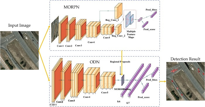
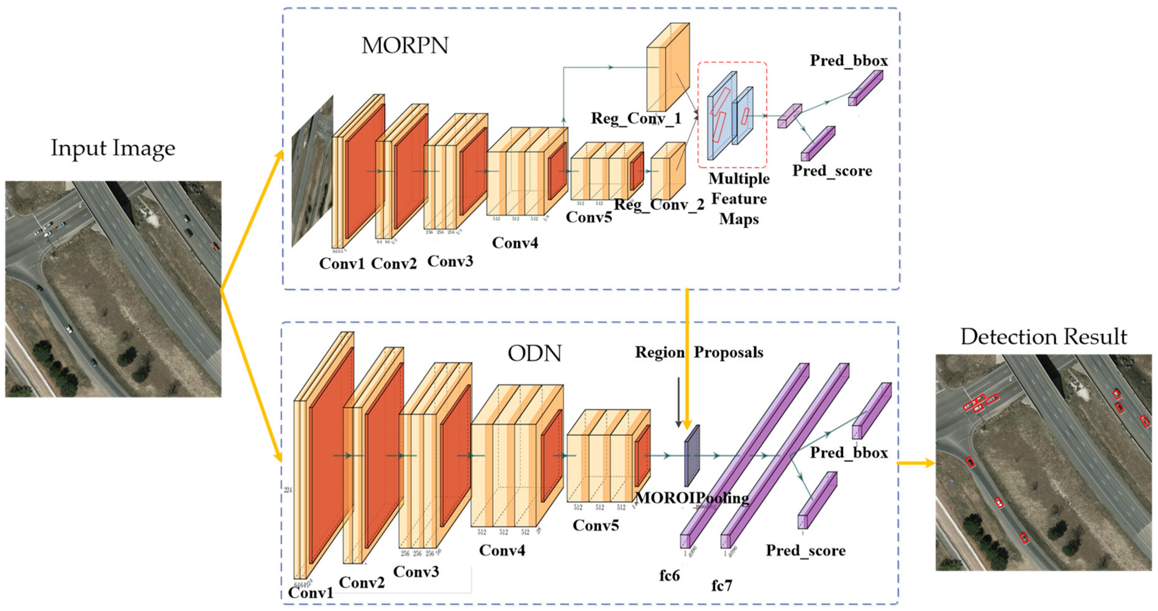
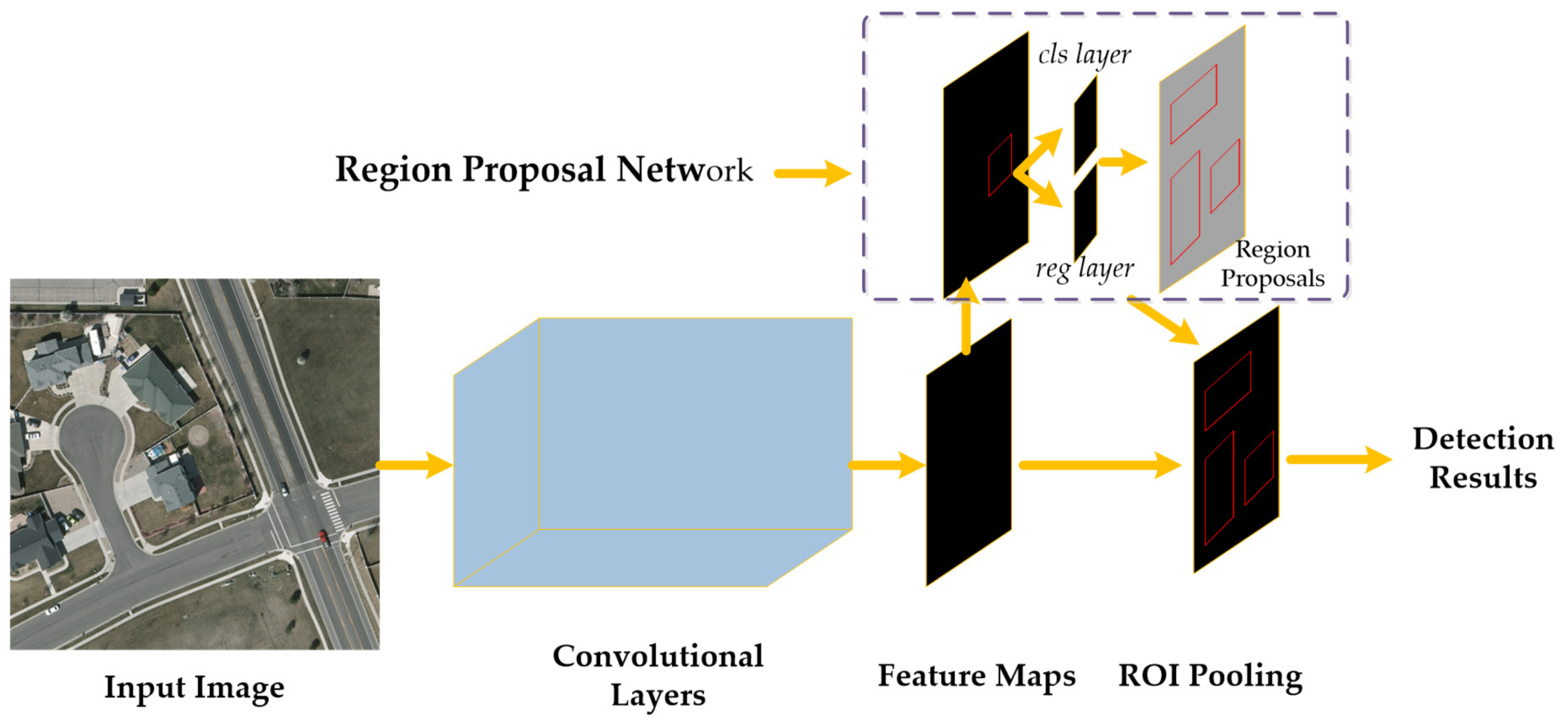
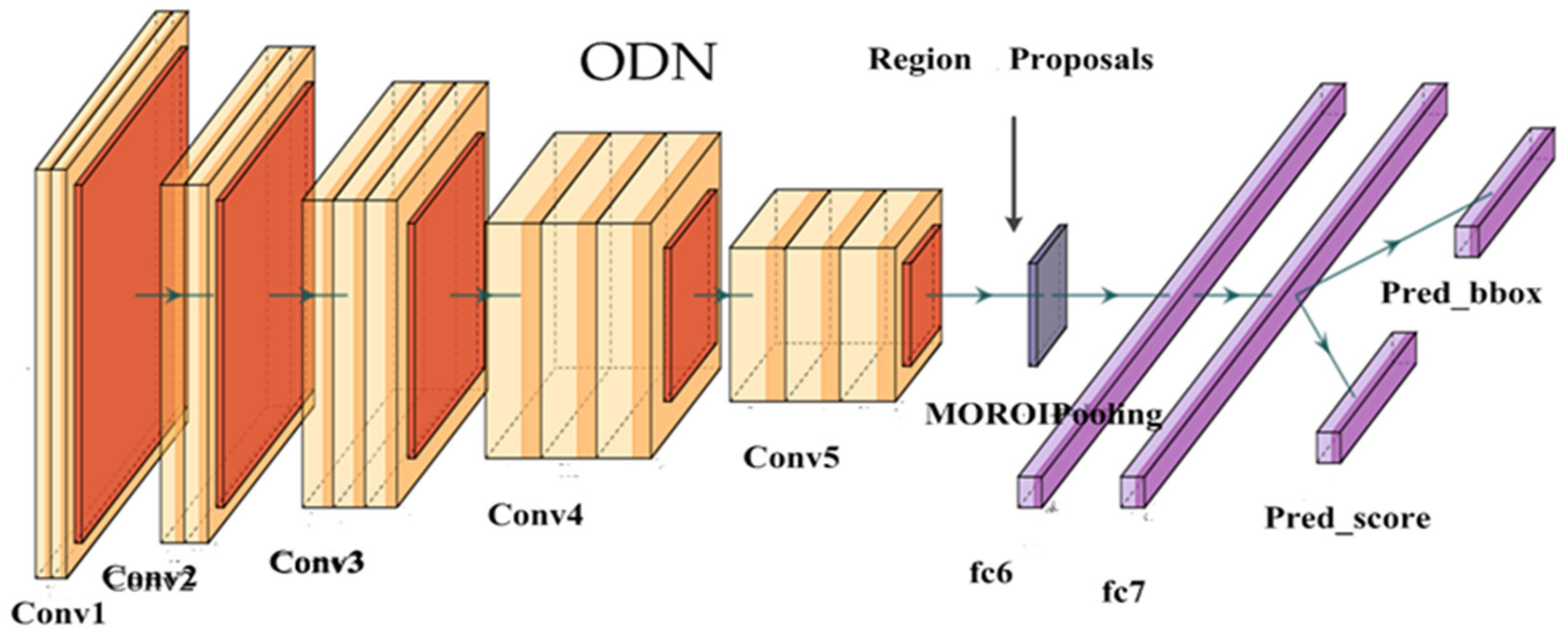
- We designed a CNN-based detection model for the objects in aerial images, which is different from the recent CNN-based models and traditional models (that adopt hand-crafted features and the sliding-window scheme). Our model consists of two independent CNNs: MORPN (multiple orientation regional proposal network) and ODN (object detection network): the MORPN is applied to generate multiple orientation region proposals, and the ODN is used to extract the features and make decisions.
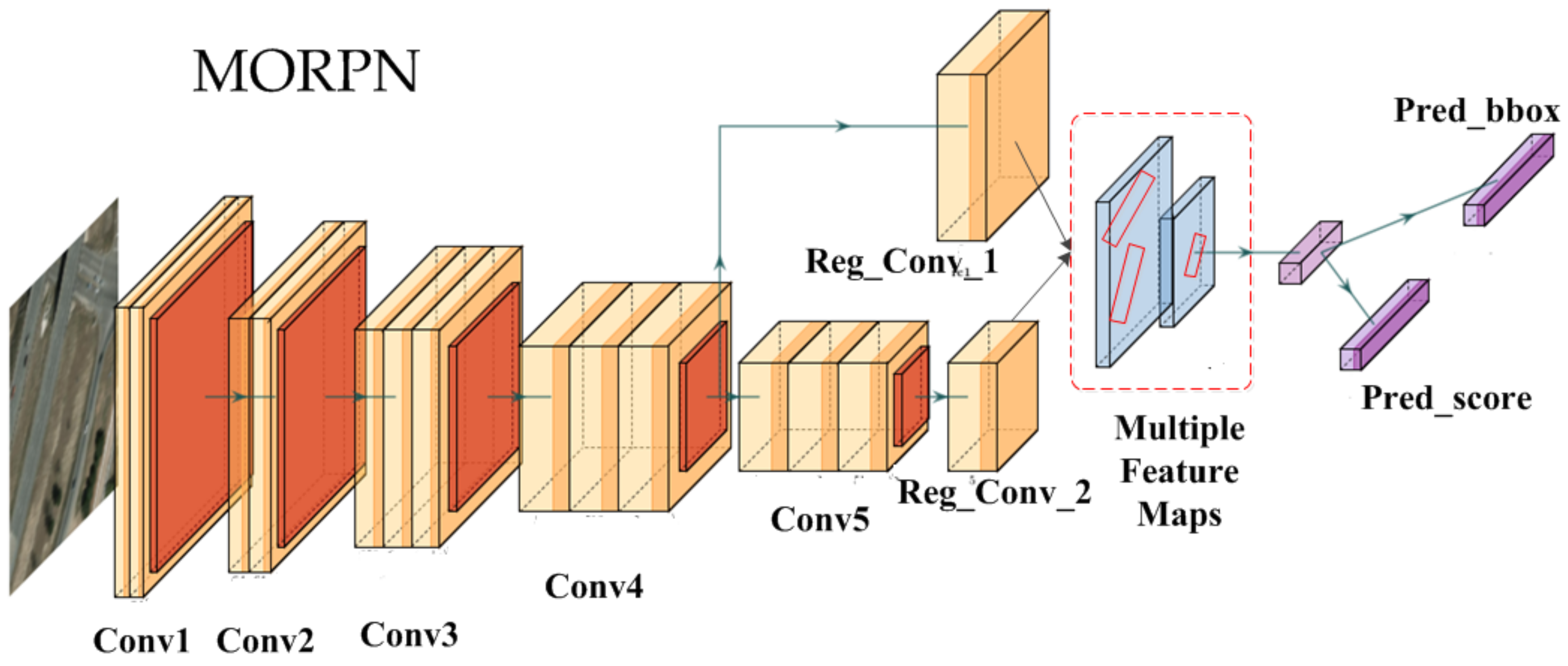
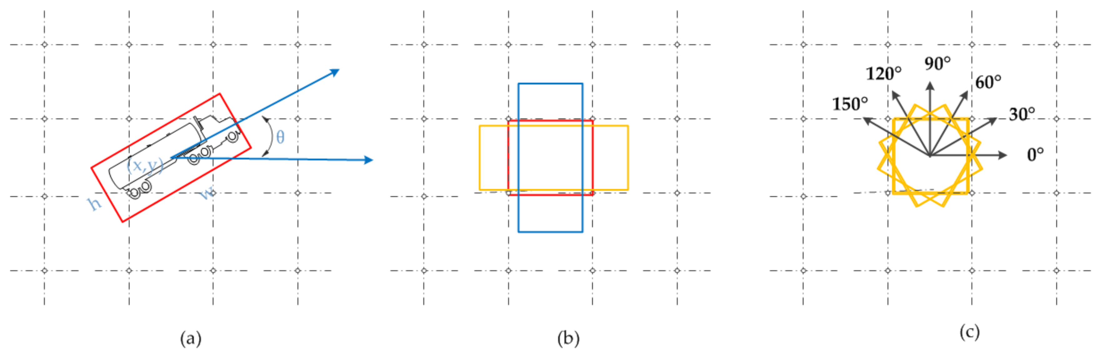
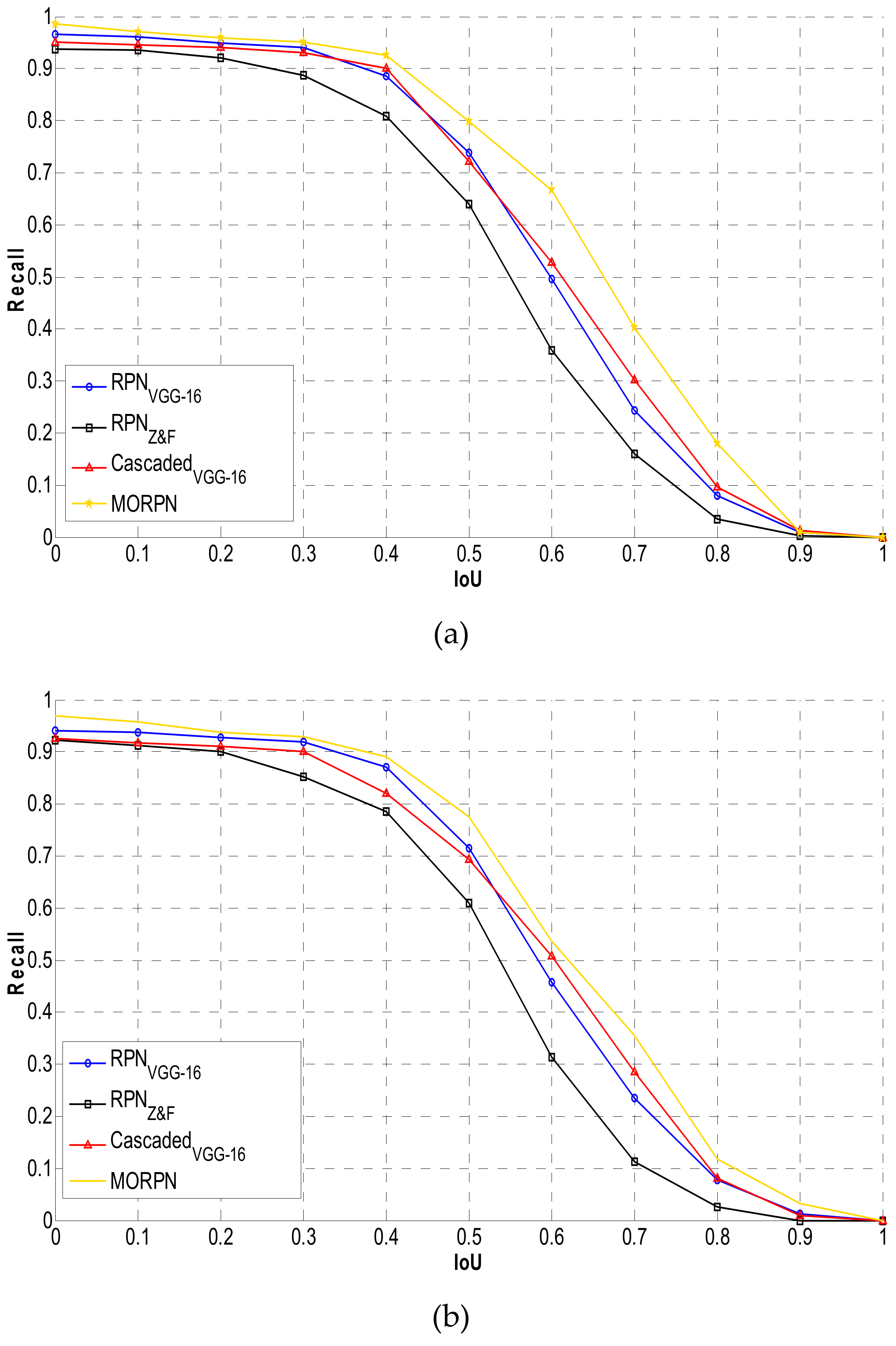
- To deal with the objects with a small size and multiple orientations in the aerial image, we proposed the MORPN. For the small-sized objects, the proposed MORPN employs a hierarchical structure that combines the feature maps of multiple scales and hierarchies to generate the region proposals. For the objects with multiple orientations, to improve the positioning accuracy, the angle information is adopted to generate the oriented candidate regions, unlike the classical CNN-based models that generate only horizontal region proposals. Moreover, an object detection network named ODN is trained to extract deep features and make decisions.
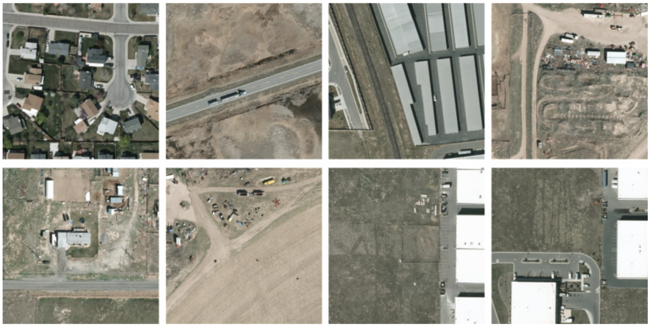
- The proposed detection model was tested on two real-world aerial image datasets: VEDAI (vehicle detection in aerial imagery) [44] and OIRDS (overhead imagery research data set) [45]. Extensive experiments were conducted, and the evaluation results indicated that the proposed model achieved significant improvement in the detection performance compared to that of its counterparts.
2. Related Work
3. Methods
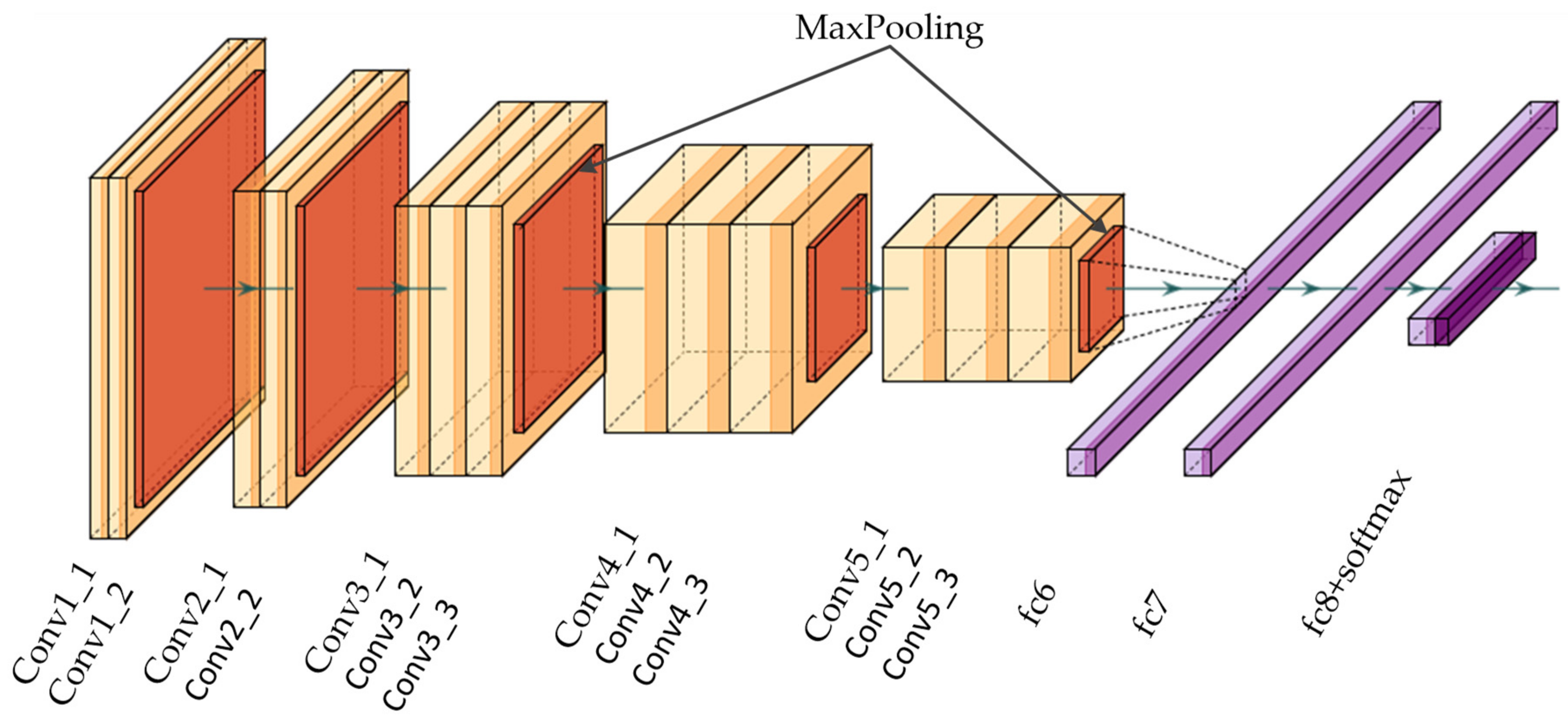
3.1. Backbone Architecture
3.2. Region Proposal Approach
3.3. MORPN
3.4. ODN
4. Experimental Results and Discussions
4.1. Evaluation Metrics
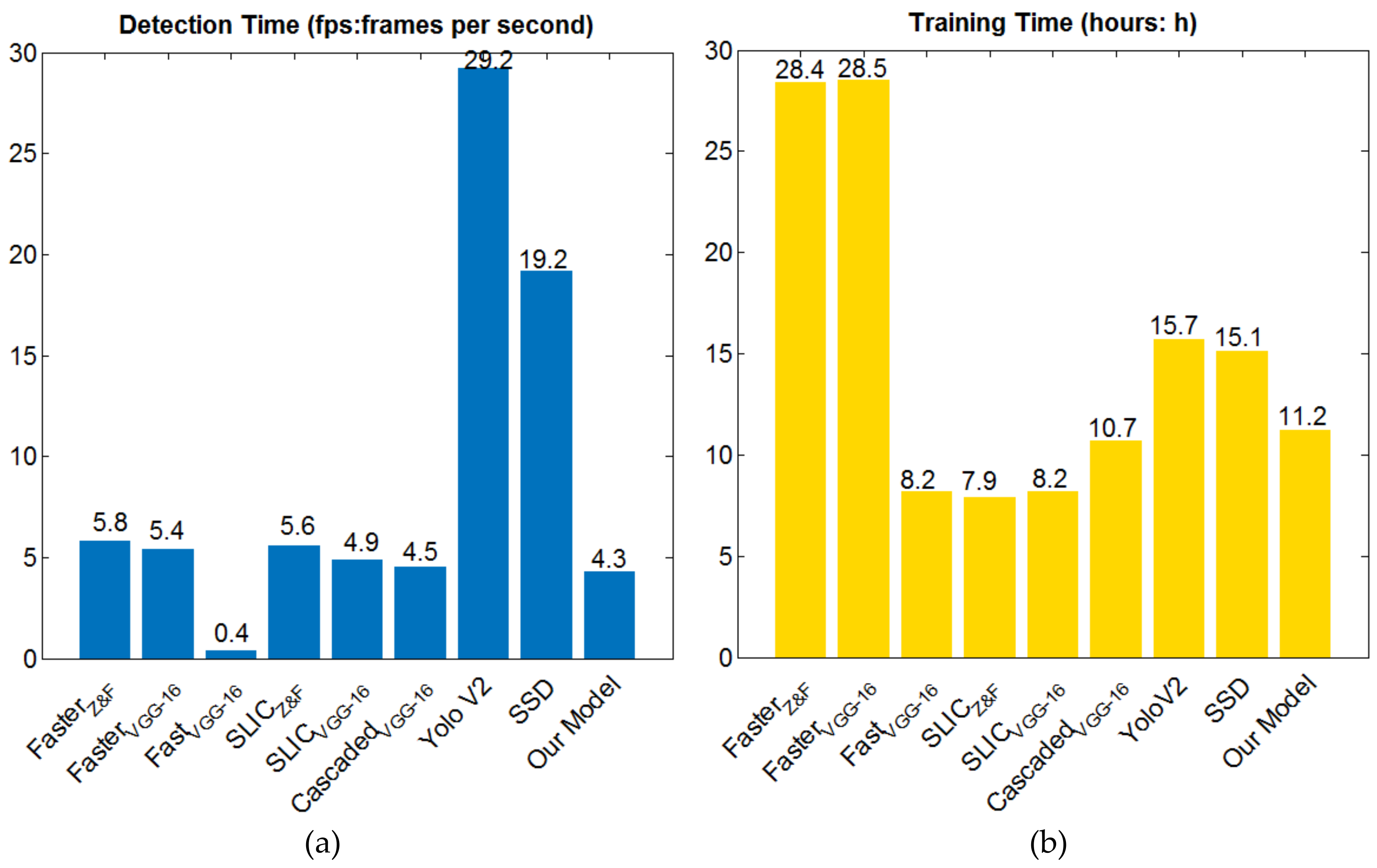
4.2. Baselines
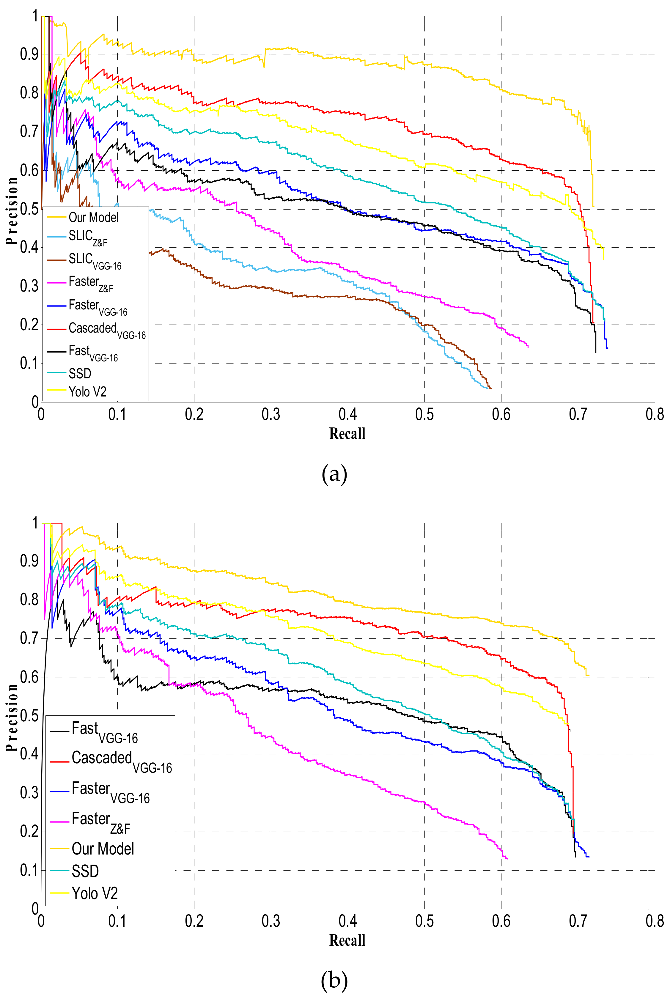
4.3. VEDAI Dataset
4.4. OIRDS
5. Conclusions
Author Contributions
Funding
Acknowledgments
Conflicts of Interest
References
- Guo, Z.; Du, S.; Zhao, W.; Lin, Y. A graph-based approach for the co-registration refinement of very-high-resolution imagery and digital line graphic data. Int. J. Remote Sens. 2016, 17, 4015–4034. [Google Scholar] [CrossRef]
- Menouar, H.; Guvenc, I.; Akkaya, K. UAV-Enabled Intelligent Transportation Systems for the Smart City: Applications and Challenges. IEEE Commun. Mag. 2017, 3, 22–28. [Google Scholar] [CrossRef]
- Gómez-Candón, D.; De Castro, A.I.; Granados, F. Assessing the accuracy of mosaics from unmanned aerial vehicle (UAV) imagery for precision agriculture purposes in wheat. Precis. Agric. 2013, 1, 44–56. [Google Scholar] [CrossRef]
- Cheng, F.; Huang, S.; Ruan, S. Scene Analysis for Object Detection in Advanced Surveillance Systems Using Laplacian Distribution Model. IEEE Trans. Syst. Man Cybern. Part C 2011, 41, 589–598. [Google Scholar] [CrossRef]
- Yin, J.; Liu, L.; Li, H. The infrared moving object detection and security detection related algorithms based on W4 and frame difference. The infrared moving object detection and security detection related algorithms based on W4 and frame difference. Infrared Phys. Technol. 2016, 77, 302–315. [Google Scholar] [CrossRef]
- Trupti, M.; Jadhav, P.M.; Phadke, A.C. Suspicious object detection in surveillance videos for security applications. In Proceedings of the International Conference on Inventive Computation Technologies (ICICT), Coimbatore, India, 26–27 August 2016; pp. 1–5. [Google Scholar]
- Dalal, N.; Triggs, B. Histograms of oriented gradients for human detection. In Proceedings of the IEEE Conference on Computer Vision and Pattern Recognition, San Diego, CA, USA, 20–25 June 2005; pp. 886–893. [Google Scholar]
- Felzenszwalb, P.; Girshick, R.; McAllester, D.; Ramanan, D. Object detection with discriminatively trained part based models. IEEE Trans. Pattern Anal. Mach. Intell. 2010, 32, 1627–1645. [Google Scholar] [CrossRef] [PubMed]
- Lin, L.; Wang, X.; Yang, W.; Lai, J. Discriminatively Trained And-Or Graph Models for Object Shape Detection. IEEE Trans. Pattern Anal. Mach. Intell. 2015, 37, 959–972. [Google Scholar] [CrossRef] [PubMed]
- Huang, S. Discriminatively trained patch-based model for occupant classification. IET Intell. Transp. Syst. 2012, 6, 132–138. [Google Scholar] [CrossRef]
- Cheng, G.; Han, J.; Guo, L.; Qian, X.; Zhou, P.; Yao, X.; Hu, X. Object detection in remote sensing imagery using a discriminatively trained mixture model. ISPRS J. Photogramm. Remote Sens. 2013, 85, 32–43. [Google Scholar] [CrossRef]
- Yao, C.; Bai, X.; Liu, W.; Latecki, L. Human Detection Using Learned Part Alphabet and Pose Dictionary. In Proceedings of the European Conference on Computer Vision, Zurich, Switzerland, 6–12 September 2014; pp. 251–266. [Google Scholar]
- Uijlings, J.; Van de Sande, K.; Gevers, T.; Smeulders, A. Selective search for object recognition. Int. J. Comput. Vis. 2013, 104, 154–171. [Google Scholar] [CrossRef]
- Cheng, M.; Zhang, Z.; Lin, W.; Torr, P. BING: Binarized Normed Gradients for Objectness Estimation at 300fps. In Proceedings of the IEEE Conference on Computer Vision and Pattern Recognition, Columbus, OH, USA, 23–28 June 2014; pp. 3286–3293. [Google Scholar]
- Alexe, B.; Deselaers, T.; Ferrari, V. Measuring the objectness of image windows. IEEE Trans. Pattern Anal. Mach. Intell. 2012, 54, 2189–2202. [Google Scholar] [CrossRef] [PubMed]
- Carreira, J.; Sminchisescu, C. CPMC: Automatic object segmentation using constrained parametric min-cuts. IEEE Trans. Pattern Anal. Mach. Intell. 2012, 34, 1312–1328. [Google Scholar] [CrossRef] [PubMed]
- Tian, W.; Zhao, Y.; Yuan, Y. Abing: Adjusted binarized normed gradients for objectness estimation. In Proceedings of the International Conference on Signal Processing, Hangzhou, China, 19–23 October 2014; pp. 1295–1300. [Google Scholar]
- Hosang, J.; Benenson, R.; Dollar, P.; Schiele, B. What makes for effective detection proposals? IEEE Trans. Pattern Anal. Mach. Intell. 2016, 38, 814–830. [Google Scholar] [CrossRef] [PubMed]
- Chavali, N.; Agrawal, H.; Mahendru, A.; Batra, D. Object-Proposal Evaluation Protocol is ‘Gameable’. In Proceedings of the IEEE International Conference on Computer Vision and Pattern Recognition, Las Vegas, NV, USA, 27–30 June 2016; pp. 2578–2586. [Google Scholar]
- Arbeláez, P.; Pont-Tuset, J.; Barron, J.; Marques, F.; Malik, J. Multiscale combinatorial grouping. In Proceedings of the IEEE International Conference on Computer Vision and Pattern Recognition, Columbus, OH, USA, 23–28 June 2014; pp. 328–335. [Google Scholar]
- Kuo, W.; Hariharan, B.; Malik, J. Deepbox: Learning objectness with convolutional networks. In Proceedings of the IEEE International Conference on Computer Vision, Santiago, Chile, 7–13 December 2015; pp. 2479–2487. [Google Scholar]
- Michael, V.; Xavier, B.; Gemma, R.; Benjamin, D. SEEDS: Superpixels extracted via energy-driven sampling. In Proceedings of the European Conference on Computer Vision, Firenze, Italy, 7–13 October 2012; pp. 13–26. [Google Scholar]
- Vedaldi, A.; Soatto, S. Quick shift and kernel methods for mode seeking. In Proceedings of the European Conference on Computer Vision, Marseille, France, 12–18 October 2008; pp. 705–718. [Google Scholar]
- Veksler, O.; Boykov, Y.; Mehrani, P. Superpixels and supervoxels in an energy optimization framework. In Proceedings of the European Conference on Computer Vision, Heraklion, Crete, Greece, 5–11 September 2010; pp. 211–224. [Google Scholar]
- Bergh, M.; Boix, X.; Roig, G.; Capitani, B.; Gool, L. SEEDS: Superpixels Extracted via Energy-Driven Sampling. Int. J. Comput. Vis. 2013, 7578, 1–17. [Google Scholar]
- Achanta, R.; Shaji, A.; Smith, K.; Lucchi, A.; Fua, P. SLIC superpixels compared to state-of-the-art superpixel methods. IEEE Trans. Pattern Anal. Mach. Intell. 2012, 34, 2274–2282. [Google Scholar] [CrossRef] [PubMed]
- Ren, S.; He, K.; Girshick, R.; Sun, J. Faster R-CNN: Towards Real-Time Object Detection with Region Proposal Networks. IEEE Trans. Pattern Anal. Mach. Intell. 2017, 39, 1137–1149. [Google Scholar] [CrossRef] [PubMed]
- Kong, T.; Yao, A.; Chen, Y.; Sun, F. HyperNet: Towards Accurate Region Proposal Generation and Joint Object Detection. In Proceedings of the IEEE Conference on Computer Vision and Pattern Recognition, Las Vegas, NV, USA, 27–30 June 2016; pp. 845–853. [Google Scholar]
- He, K.; Zhang, X.; Ren, S.; Sun, J. Spatial Pyramid Pooling in Deep Convolutional Networks for Visual Recognition. IEEE Trans. Pattern Anal. Mach. Intell. 2015, 37, 1904–1916. [Google Scholar] [CrossRef] [PubMed]
- Zitnick, C.; Dollár, P. Edge Boxes: Locating Object Proposals from Edges. In Proceedings of the European Conference on Computer Vision, Zurich, Switzerland, 6–12 September 2014; pp. 391–405. [Google Scholar]
- Cai, Z.; Fan, Q.; Rogerio, S.; Vasconcelos, F. A Unified Multi-Scale Deep Convolutional Neural Network for Fast Object Detection. In Proceedings of the European Conference on Computer Vision, Amsterdam, The Netherlands, 11–14 October 2016; pp. 354–370. [Google Scholar]
- Li, J.; Liang, X.; Shen, S.; Xu, T.; Feng, J.; Yan, S. Scale-Aware Fast R-CNN for Pedestrian Detection. IEEE Trans. Multimed. 2018, 20, 985–996. [Google Scholar] [CrossRef]
- Lowe, D. Distinctive image features from scale-invariant keypoints. Int. J. Comput. Vis. 2004, 60, 91–110. [Google Scholar] [CrossRef]
- Bay, H.; Tuytelaars, T.; Gool, L. SURF: Speeded Up Robust Features. In Proceedings of the European Conference on Computer Vision, Graz, Austria, 7–13 May 2006; pp. 404–417. [Google Scholar]
- Krizhevsky, A.; Sutskever, I.; Hinton, G. ImageNet classification with deep convolutional neural networks. In Proceedings of the 25th International Conference on Neural Information Processing System, Lake Tahoe, NV, USA, 3–6 December 2012. [Google Scholar]
- Deng, J.; Berg, A.; Satheesh, S.; Su, H.; Khosla, A.; Li, F. ImageNet Large Scale Visual Recognition Competition 2012 (ILSVRC2012). Available online: http://www.image-net.org/challenges/LSVRC/2012 (accessed on 1 May 2019).
- Zeiler, M.; Fergus, R. Visualizing and Understanding Convolutional Networks. In Proceedings of the European Conference on Computer Vision, Zurich, Switzerland, 6–12 September 2014; pp. 818–833. [Google Scholar]
- Simonyan, K.; Zisserman, A. Very deep convolutional networks for large-scale image recognition. arXiv 2014, arXiv:1409.1556. [Google Scholar]
- Szegedy, C.; Liu, W.; Jia, Y. Going deeper with convolutions. In Proceedings of the IEEE Conference on Computer Vision and Pattern Recognition, Boston, MA, USA, 7–12 June 2015; pp. 1–9. [Google Scholar]
- Redmon, J.; Divvala, S.; Girshick, R.; Farhadi, A. You Only Look Once: Unified, Real-Time Object Detection. arXiv 2015, arXiv:1506.02640. [Google Scholar]
- Liu, W.; Anguelov, D.; Erhan, D.; Szegedy, C.; Reed, S.; Fu, C. SSD: Single Shot MultiBox Detector. In Proceedings of the European Conference on Computer Vision, Amsterdam, The Netherlands, 11–14 October 2016; pp. 21–37. [Google Scholar]
- Redmon, J.; Farhadi, A. YOLO9000: Better, Faster, Stronger. In Proceedings of the IEEE Conference on Computer Vision and Pattern Recognition (CVPR), Honolulu, HI, USA, 21–26 July 2017; pp. 6517–6525. [Google Scholar]
- Xie, H.; Wang, T.; Qiao, M.; Zhang, M.; Shan, G.; Snoussi, H. Robust object detection for tiny and dense targets in VHR aerial images. In Proceedings of the Chinese Automation Congress (CAC), Jinan, China, 20–22 October 2017; pp. 6397–6401. [Google Scholar]
- Razakarivony, S.; Jurie, F. Vehicle detection in aerial imagery: A small target detection benchmark. J. Vis. Commun. Image Represent. 2016, 34, 187–203. [Google Scholar] [CrossRef]
- Tanner, F.; Colder, B.; Pullen, C.; Heagy, D.; Eppolito, M.; Carlan, V.; Oertel, C.; Sallee, P. Overhead imagery research data set—An annotated data library & tools to aid in the development of computer vision algorithms. In Proceedings of the IEEE Applied Imagery Pattern Recognition Workshop, Washington, DC, USA, 14–16 October 2009; pp. 1–8. [Google Scholar]
- Xu, Y.; Yu, G.; Wang, Y.; Wu, X.; Ma, Y. A Hybrid Vehicle Detection Method Based on Viola-Jones and HOG + SVM from UAV Images. Sensors 2016, 16, 1325. [Google Scholar] [CrossRef] [PubMed]
- Ammour, N.; Alhichri, H.; Bazi, Y.; Benjdira, B.; Alajlan, N. Deep Learning Approach for Car Detection in UAV Imagery. Remote Sens. 2017, 9, 312. [Google Scholar] [CrossRef]
- Qu, T.; Zhang, Q.; Sun, S. Vehicle detection from high-resolution aerial images using spatial pyramid pooling-based deep convolutional neural networks. Multimed. Tools Appl. 2016. [Google Scholar] [CrossRef]
- Tang, T.; Zhou, S.; Deng, Z.; Zou, H.; Lei, L. Vehicle Detection in Aerial Images Based on Region Convolutional Neural Networks and Hard Negative Example Mining. Sensors 2017, 17, 336. [Google Scholar] [CrossRef] [PubMed]
- Deng, Z.; Sun, H.; Zhou, S.; Zhao, J.; Zou, H. Toward Fast and Accurate Vehicle Detection in Aerial Images Using Coupled Region-Based Convolutional Neural Networks. IEEE J. Sel. Top. Appl. Earth Obs. Remote Sens. 2017, 10, 3652–3664. [Google Scholar] [CrossRef]
- Wang, G.; Wang, X.; Fan, B.; Pan, C. Feature Extraction by Rotation-Invariant Matrix Representation for Object Detection in Aerial Image. IEEE Geosci. Remote Sens. Lett. 2017, 14, 851–855. [Google Scholar] [CrossRef]
- Zheng, Z.; Zhou, G.; Wang, Y.; Liu, Y.; Li, X.; Wang, X.; Jiang, L. A Novel Vehicle Detection Method with High Resolution Highway Aerial Image. IEEE J. Sel. Top. Appl. Earth Obs. Remote Sens. 2013, 6, 2338–2343. [Google Scholar] [CrossRef]
- Ševo, I.; Avramović, A. Convolutional Neural Network Based Automatic Object Detection on Aerial Images. IEEE Geosci. Remote Sens. Lett. 2016, 13, 740–744. [Google Scholar] [CrossRef]
- Yan, J.; Wang, H.; Yan, M.; Diao, W.; Sun, X.; Li, H. IoU-Adaptive Deformable R-CNN: Make Full Use of IoU for Multi-Class Object Detection in Remote Sensing Imagery. Remote Sens. 2019, 11, 286. [Google Scholar] [CrossRef]
- Al-Najjar, H.; Kalantar, B.; Pradhan, B.; Saeidi, V.; Halin, A.; Ueda, N.; Mansor, S. Land Cover Classification from fused DSM and UAV Images Using Convolutional Neural Networks. Remote Sens. 2019, 11, 1461. [Google Scholar] [CrossRef]
- Zhong, J.; Lei, T.; Yao, G. Robust Vehicle Detection in Aerial Images Based on Cascaded Convolutional Neural Networks. Sensors 2017, 17, 2720. [Google Scholar] [CrossRef]
- Girshick, R. Fast R-CNN. In Proceedings of the IEEE International Conference on Computer Vision, Santiago, Chile, 7–13 December 2015; pp. 1440–1448. [Google Scholar]
- Plaisted, D.; Hong, J. A heuristic triangulation algorithm. J. Algorithms 1987, 8, 405–437. [Google Scholar] [CrossRef]
- Kahaki, S.; Nordin, M.; Ashtari, A.; Zahra, S. Invariant Feature Matching for ImageRegistration Application Based on New Dissimilarity of Spatial Features. PLoS ONE 2016, 11, e0149710. [Google Scholar]
- Qin, T.; Liu, T.; Li, H. A general approximation framework for direct optimization of information retrieval measures. Inf. Retr. 2010, 4, 375–397. [Google Scholar] [CrossRef]


| For an input-oriented region proposal defined by (x, y, h, w, θ) with a spatial scale Sa 1. Calculate the sub-region size: 2. Find the top-left coordinate of each sub-region as follows: Where, 3. Calculate the rotated coordinate of (x0, y0) by using Equation (5) (presented below) 4. Perform max-pooling on each sub-region a. set v = 0; b. compare the value of the feature map with v at each position (px, py) by using Equation (6) (presented below) c. set v as the max value of this region d. set the position (i,j) of the output feature map as Feature(i,j) = v 5. Repeat the steps from 2 to 5 until the Feature(i,j) at each sub-region is calculated. |
| Type | Tag | Number | Type | Tag | Number | Type | Tag | Number |
|---|---|---|---|---|---|---|---|---|
| Car | car | 1340 | Plane | pla | 47 | Tractor | tra | 190 |
| Pick-up | pic | 950 | Boat | boa | 170 | Van | van | 100 |
| Truck | tru | 300 | Camping car | cam | 390 | Other | oth | 200 |
| Parameter | Value |
|---|---|
| Weight decay | 0.0005 |
| Momentum | 0.9 |
| Iterations | 40,000 |
| Learning rate | first 30,000 iters: 0.001 remaining 10,000 iters: 0.0001 |
| Evaluation Metric | VEDAI 1024 | ||||||||
|---|---|---|---|---|---|---|---|---|---|
| FastVGG-16 | FasterVGG-16 | FasterZ&F | SLIC VGG-16 | SLICZ&F | Cascaded VGG-16 | SSD [41] | Yolo V2 [42] | Our Model | |
| Recall Rate | 72.2% | 73.9% | 63.5% | 58.8% | 58.3% | 72.3% | 70.5% | 73.8% | 75.1% |
| AP | 39.8% | 42.1% | 30.8% | 23.2% | 25.4% | 54.6% | 46.1% | 50.3% | 63.2% |
| F1-Score | 0.229 | 0.232 | 0.216 | 0.064 | 0.066 | 0.320 | 0.295 | 0.313 | 0.469 |
© 2019 by the authors. Licensee MDPI, Basel, Switzerland. This article is an open access article distributed under the terms and conditions of the Creative Commons Attribution (CC BY) license (http://creativecommons.org/licenses/by/4.0/).
Share and Cite
Chen, C.; Zhong, J.; Tan, Y. Multiple-Oriented and Small Object Detection with Convolutional Neural Networks for Aerial Image. Remote Sens. 2019, 11, 2176. https://doi.org/10.3390/rs11182176
Chen C, Zhong J, Tan Y. Multiple-Oriented and Small Object Detection with Convolutional Neural Networks for Aerial Image. Remote Sensing. 2019; 11(18):2176. https://doi.org/10.3390/rs11182176
Chicago/Turabian StyleChen, Chao, Jiandan Zhong, and Yi Tan. 2019. "Multiple-Oriented and Small Object Detection with Convolutional Neural Networks for Aerial Image" Remote Sensing 11, no. 18: 2176. https://doi.org/10.3390/rs11182176
APA StyleChen, C., Zhong, J., & Tan, Y. (2019). Multiple-Oriented and Small Object Detection with Convolutional Neural Networks for Aerial Image. Remote Sensing, 11(18), 2176. https://doi.org/10.3390/rs11182176