Ocean Color Quality Control Masks Contain the High Phytoplankton Fraction of Coastal Ocean Observations

Abstract

Satellite estimation of oceanic chlorophyll-a content has enabled characterization of global phytoplankton stocks, but the quality of retrieval for many ocean color products (including chlorophyll-a) degrades with increasing phytoplankton biomass in eutrophic waters. Quality control of ocean color products is achieved primarily through the application of masks based on standard thresholds designed to identify suspect or low-quality retrievals. This study compares the masked and unmasked fractions of ocean color datasets from two Eastern Boundary Current upwelling ecosystems (the California and Benguela Current Systems) using satellite proxies for phytoplankton biomass that are applicable to satellite imagery without correction for atmospheric aerosols. Evaluation of the differences between the masked and unmasked fractions indicates that high biomass observations are preferentially masked in National Aeronautics and Space Administration (NASA) ocean color datasets as a result of decreased retrieval quality for waters with high concentrations of phytoplankton. This study tests whether dataset modification persists into the default composite data tier commonly disseminated to science end users. Further, this study suggests that statistics describing a dataset’s masked fraction can be helpful in assessing the quality of a composite dataset and in determining the extent to which retrieval quality is linked to biological processes in a given study region.

1. Introduction

Ocean color remote sensing has greatly improved our ability to monitor global scale biological processes of ocean systems [1,2] but the potential for conventional satellite ocean color tools to characterize coastal ecosystems is limited by the assumptions used in various algorithms, for example that diverse phytoplankton communities match global bio-optical relationships [3] or that backscattered light from particles does not interfere with atmospheric correction [4]. Although these assumptions are often not valid for coastal waters [5], satellite assessment of coastal marine ecosystems is an area of intense focus in part because of reported increases in the frequency of coastal phytoplankton blooms considered harmful to humans and wildlife [6,7,8,9,10]. Fundamental challenges for ocean color remote sensing of coastal marine ecosystems arise from the increased complexity of water constituents, as well as the entanglement of atmospheric and oceanic signals. Overcoming these difficulties motivates next-generation ocean color satellite missions, with the aim to characterize oceanic ecosystems spanning oligotrophic to eutrophic waters, for example through increasing spectral resolution to resolve variability in phytoplankton pigmentation [11] and through increasing spectral range to discern the effects of absorbing aerosols and colored dissolved organic matter and to improve aerosol characterization [12]. Nonetheless, data from existing satellite platforms is presently required to assess coastal marine ecosystems. When next-generation sensing platforms become operational, interpreting legacy measurements of coastal waters will still be necessary in order to construct and interpret climate-quality data records and will require methods to detect regional bias of legacy retrievals [13,14,15]. For coastal targets, constructing climate-quality datasets will require an approach to maintain atmospheric correction efficacy across variable phytoplankton concentrations.

Conventional approaches for atmospheric correction of ocean color satellite imagery take advantage of the strong light absorption by water at longer wavelengths, for example, in the near-infrared (NIR), to estimate that the water-leaving radiance (L_W) in the NIR (L_W(NIR)) is negligible [16]. Thus, after removal of glint and white capping effects, the derived top-of-atmosphere (TOA) radiance in the NIR (L_TOA(NIR)) is attributed to the atmospheric contributions by Rayleigh scattering, aerosol scattering and multiple interactions between Rayleigh and aerosol scattering [17], allowing a solution to discern aerosol thickness.

The approximation that L_W(NIR) is zero, termed the “Black Pixel Assumption” [4], is often incorrect, frequently so in coastal waters where high near-surface particle loads (organic or inorganic) can strongly backscatter light, such that the L_W(NIR) domain is appreciably non-zero. Because L_TOA(NIR) is attributed to atmospheric constituents, L_W(NIR) contributions cause overestimation of backscattering by atmospheric aerosols and thus result in incorrect (often negative) derivation of L_W in the visible domain (L_W(VIS)), particularly in the blue bands used for, among others, chlorophyll-a derivation [18]. As a result, atmospheric correction is more problematic for water masses with high particle loads, including of phytoplankton cells and high biomass pixels are frequently removed during quality control processing of satellite datasets (Figure 1).

Alternate atmospheric correction methods have been developed with the goal of improving L_W(VIS) retrieval in coastal waters, for example by estimating aerosol contributions from longer (short-wave infrared) bands [19], by assuming stable NIR reflectance ratios within a scene [20] or by neural network determination of atmospheric contribution [21]. Alternate methods for atmospheric correction of coastal imagery have generally improved performance of nearshore ocean color retrievals compared with the conventional (NIR-based) methodology [22], although users still must decide when use of these methods is preferable given tradeoffs of noisy wavebands, non-analytical solutions and increased difficulty in obtaining alternate processing for National Aeronautics and Space Administration (NASA) imagery. Another potential reason for usage of default NIR aerosol corrected imagery, evaluated in detail within this work, is that the alteration of satellite dataset distributions by atmospheric correction errors may be obscured by the default quality control masks applied to composited imagery.

Quality control of NASA ocean color imagery is achieved in part through flag assignments that trigger masking or removal of individual pixels which do not satisfy pre-defined thresholds. Increasingly rigorous flag criteria are applied to mask observations from sequential data tiers, based on the quality requirements of the tier’s expected end-users. Pixels within atmospherically-corrected imagery (level 2 data tier, L2) are masked by default when the derivation of meaningful products is severely inhibited, for example when the sensor is viewing land or clouds or when the sensor saturates. L2 datasets contain shifting pixel coordinates, frequent data gaps (i.e., from clouds) and large file sizes inconvenient for users requiring continuous or less computationally expensive products [23]. To satisfy these user needs, statistical composites of geophysical variables binned in space and time (level 3 data tier, L3) are provided by the NASA Ocean Biology Processing Group (OBPG) and are valuable to users beyond the ocean color community, for example as inputs into biogeochemical models. In order to provide higher quality composites for a larger end-user community, the default masks applied during L3 processing are more rigorous than during L2 processing, for example removing observations flagged for likely or known errors in atmospheric correction. Spatial distortions may also arise during compositing and although not evaluated here, are likewise relevant to L3 end-users [24].

In this study, we compare estimates of phytoplankton biomass obtained without aerosol correction for observations that satisfy (versus fail) standard quality control thresholds for two Eastern Boundary Current (EBC) ecosystems. Characterization of the changes that occur from removing portions of satellite datasets enables assessment of whether quality control methodology alters satellite perspectives of biology in coastal ecosystems. We assess whether observations that satisfy quality control methods—hereafter the masked fraction—provide an unbiased perspective of phytoplankton biomass in coastal ecosystems and we provide examples for L3 end-users to consider when determining whether use of standard composite products may be reasonable for a specific study region.

2. Materials and Methods

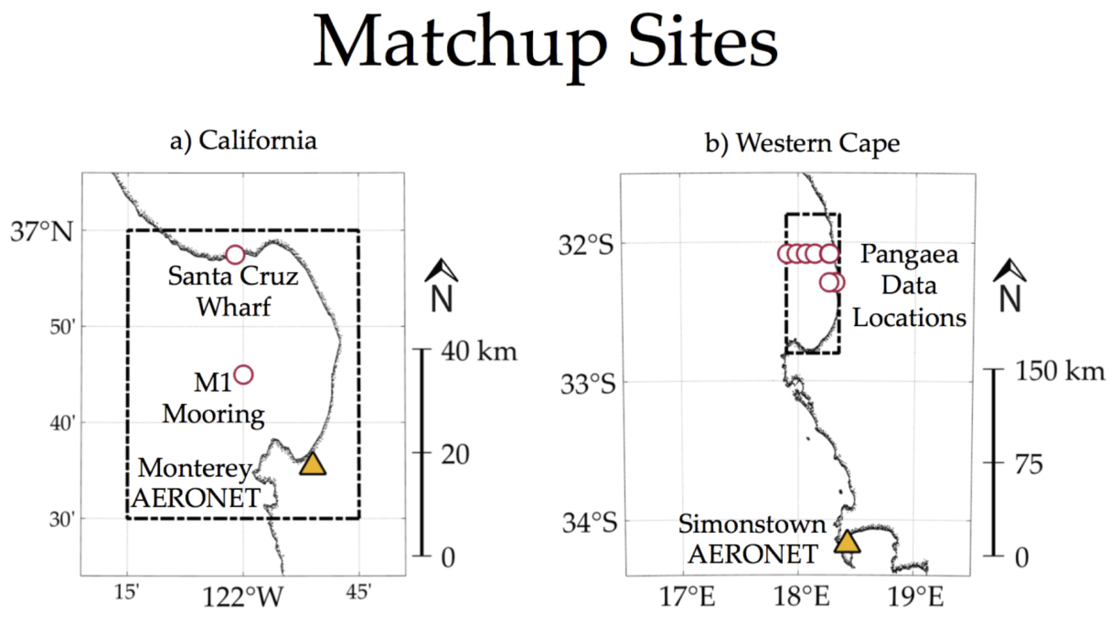
2.1. Site Selection:

The mid-latitude eastern margins (or EBCs) of the world’s oceans are regions of heightened biological primary production due to coastal upwelling or the wind-driven transport of nutrient-rich subsurface waters to the illuminated surface layer. Heightened nutrient availability, coupled with the persistence of seed stocks from the shelf and from retention in the lee of headlands, support high phytoplankton concentrations that periodically form blooms, some of which may be harmful to humans and wildlife [7,25].

Here we consider EBC ecosystems of Monterey Bay (MB), California, USA and St. Helena Bay (SHB), Western Cape, South Africa. MB is within a marine sanctuary and is partially sheltered from the predominant alongshore winds of the central California Current System (CCS) by coastline geometry. Phytoplankton in the region follow a distinct climatology, with spring onset of upwelling-favorable winds supporting diatom-rich phytoplankton blooms, followed by a mid-summer reduction in phytoplankton associated with rapid advection to offshore waters [26]. Fall relaxation of upwelling-favorable winds and the resulting increased vertical stratification of the surface layer facilitates a community shift towards dinoflagellates, which periodically form dense red tides with concentrations that may reach or exceed those of spring diatom blooms [25].

SHB is an upwelling ecosystem in the lee of Cape Columbine within the southern Benguela Current System (BCS). The region’s proximity to the Cape Peninsula upwelling cell, coupled with shelter from the lee and a widened shelf, provides high nutrient loads in a relatively stable environment, which support persistently high phytoplankton production [27]. In addition, sea surface temperature is relatively high within SHB compared with other EBCs, allowing elevated phytoplankton populations to persist throughout all seasons [28]. As with MB, phytoplankton succession in the southern BCS, including within SHB, is dictated by the intensification and relaxation of alongshore winds, with characteristic diatom and dinoflagellate regimes dominating in the spring and fall, respectively [29].

2.2. Atmospheric Dataset:

Climatological datasets for Ångstrom exponent and aerosol optical depth (500 nm) were obtained from the Aerosol Robotic Network (AERONET; aeronet.gsfc.nasa.gov) for Monterey, California, USA (36.59°N, 121.85°W) and Simonstown, Western Cape, South Africa (34.18°S, 18.43°E; Figure 2). The Monterey AERONET site is located to the southeast of MB and separated from a nearby agricultural region by a coastal mountain range, although diurnal sea breeze north of this range may increase mixing between terrestrial and marine airmasses. The Simonstown AERONET site is located on the eastern slope of the Cape Peninsula, roughly 150 km south of Cape Columbine. Predominant windstress is equatorward (towards SHB) with summertime intensification [30].

2.3. Biological Field Data

Weekly fluorometric Chlorophyll-a (Chla) measurements (in vitro) were obtained from the Southern California Coastal Ocean Observing System portal (sccoos.org/data/habs/) for the Santa Cruz Wharf (SCW; 36.958°N, 122.017°W; Figure 2) in northern MB. Daily mean in situ surface (1 m) fluorescence measurements were obtained from a HydroScat-2 fluorometer (HOBI Labs) mounted on an oceanographic mooring in central MB (M1; 36.750°N, −122.000°E), maintained by the Monterey Bay Aquarium Research Institute (MBARI; mbari.org). Measurements of Chla within SHB were obtained from the European Space Agency (ESA) Ocean Color Climate Change Initiative (OC-CCI) dataset, available on the Pangaea portal (doi.pangaea.de). Only fluorometric measurements (in vitro) were used for match-ups with satellite products for SHB since the majority of Chla estimates in the database were based on that methodology.

2.4. Satellite Data

MODIS Aqua (MODISA) calibrated, non-atmospherically corrected imagery (L1A) was obtained from the NASA Ocean Color website (oceancolor.gsfc.nasa.gov) for dates spanning July 2002 to September 2018 within MB (36.50–37.00°N; 121.75–122.25°W) and SHB (31.80–32.80°S; 17.90–18.35°E; Figure 2) for matchup validation and for analysis of L2 datasets. Surface reflectances (${\rho }_S$) were obtained for both regions from geo-referenced and atmospherically corrected imagery produced using NASA OBPG software SeaDAS (version 7.5) with observations removed if viewing land or clouds or for non-physical retrievals (i.e., ${\rho }_S$ outside of the range 0–1). Spatial subsets used for comparison with AERONET results were selected from the MB and SHB domains based on the AERONET site location and the local topography (MB latitude < 36.65°N; longitude < 121.92°W; SHB latitude > 32.10°S; longitude > 18.10°E). Data for L3 analysis was obtained for the same timeframe and for similar regions in MB (36.50–37.00°N; 121.75–122.25°W) and SHB (32.20–32.80°S; 17.90–18.35°E), as well as for two nearby transects placed in regions with relatively north-south coastline of the CCS (37.10–37.50°N, 122.40–123.40°W) and BCS (31.80–32.20°S, 17.30–18.35°E). Processing for the L3 products applied additional SeaDAS software l2bin and l2mapgen to form daily, 4km standard map grid composites.

Quality control flags were assigned to all pixels during the L2 processing chain according to standard OBPG L2 flag thresholds. Masks were applied to one identical set of the L2 data if flag assignments indicated likely errors in atmospheric correction. Flags chosen included warnings for low water-leaving radiance (LOWLW), maximum iterations exceeded during atmospheric correction processing (MAXAERITER) and out-of-range spectral slope of derived aerosol radiances (ATMWARN). This combination of flags will be hereafter referred to as AC flags. More detailed information on thresholds and applications of default flags can be found in SeaWiFS postlaunch documentation [31].

Neural network Chla estimates were included for evaluating satellite products using processing tools provided by the Coast Color project (coastcolour.org). In short, MODISA imagery was georeferenced and calibrated using SeaDAS. Atmospheric correction and derivation of Chla was then performed using the Sentinel Application Platform (SNAP; step.esa.int) with the Case-2 Regional Coast Color (C2RCC; brockmann-consult.de) plugin.

2.5. Remote Estimation of Phytoplankton Biomass:

Remote measurements of the spectral radiance anomaly generated by sun-induced fluorescence of the Chla molecule have been applied as a proxy for phytoplankton biomass for over four decades [32,33]. The fluorescence line height approach (FLH), which subtracts a red to NIR baseline from the Chla fluorescence peak to correct for brightness effects, is the most widely used of these satellite tools. FLH has been proposed to complement traditional Chla satellite algorithms in high–biomass coastal waters [34,35] and is disseminated in standard L2 and L3 OBPG data derived from normalized L_W (nFLH). Another FLH-type method, the red band difference algorithm (RBD) [36], subtracts the signal derived at the nearest shorter wavelength from the signal measured at the Chla fluorescence peak. RBD was chosen for this work because of its relative robustness to sediment effects [36].

Fluorescence line height products, including RBD, may be derived at TOA, thus bypassing the potential errors arising during the atmospheric correction procedure. Here we use a partial atmospheric correction product that accounts for Rayleigh but not aerosol effects, termed the surface reflectance (${\rho }_S\left(\lambda \right)$), which may be defined as

$${\rho }_S\left(\lambda \right)=\left(\frac{\pi }{F_0{\mu }_0}\right)\left(\frac{L_{TOA}}{t_{solar}{t}_{sensor}}-L_r\right){\left(t{{}^{\prime }}_{solar}t{{}^{\prime }}_{sensor}t{{}^{\prime }}_{O_2}t{{}^{\prime }}_{H_{2}O}\right)}^{-1}$$

(1)

where $F_0$ is the solar downward irradiance, ${\mu }_0$ is the cosine of the solar zenith angle, $t$ and $t{}^{\prime }$ are the direct and diffuse atmospheric transmittances, respectively, for the sun-surface and surface-sensor path lengths and for the atmospheric effects of oxygen and water vapor. RBD is thus derived as the difference between MODISA surface reflectances:

$$RBD={\rho }_S\left(678nm\right)-{\rho }_S\left(667nm\right)$$

(2)

where ${\rho }_S\left(678nm\right)$ corresponds to the height of the Chla fluorescence maximum (approximately $683nm$) and ${\rho }_S\left(667nm\right)$ provides an adjacent baseline to account for overall spectral brightness.

2.6. Match-up Procedure, Derivation of Climatological Averages and Error Statistics

Validation statistics for all satellite products were derived using only same-day, 3×3 pixel median match-ups centered on the in-water samples due to high spatial and temporal variability at the match-up sites. OC3M and C2RCC, as well as fluorescence and Chla measured in situ were log₁₀-transformed prior to derivation of matchups. RBD and flag climatologies were derived as the mean monthly values for each region. Composite datasets were compared using standardized bias (SB), derived as the absolute bias due to masking of the composite data normalized by the standard deviation:

$$SB\left(i\right)=\left(\frac{{\overline{X}}_i-{\overline{Y}}_i}{{\sigma }_Y}\right)$$

(3)

where ${\overline{X}}_i$ and ${\overline{Y}}_i$ correspond to the mean composite RBD values for datasets with AC flagged pixels omitted and retained, respectively, normalized by the standard deviation of the dataset with AC flagged pixels retained (${\sigma }_Y$). $SB$ was partitioned ($i$) by longitude or by the fraction of underlying pixels (L2) which were assigned AC flags before spatial binning.

3. Results

3.1. Association Between Red Band Difference and Phytoplankton Biomarkers

Satellite match-ups at both MB and SHB indicate that the RBD algorithm associated more strongly (based on a Pearson test) with in situ proxies for phytoplankton concentrations than either a standard NASA blue-green Chla algorithm (OC3M) or a neural-network-based Chla algorithm (Coast Color), although the comparison presented here is not intended as a rigorous inter-comparison of Chla algorithms. An attempt to model surface Chla from satellite measurements (using a linear, least squares approach) resulted in generally higher (never lower) accuracy of the RBD method versus the other remote products, suggesting that RBD is a useful proxy for Chla within our study regions. Greater frequency of valid match-ups were possible at the M1 buoy (MB) location because of increased distance from land and because of the greater number of in situ records. More valid match-ups were also possible for RBD versus OC3M because the ${\rho }_S$ derivation (which does not account for aerosols) avoided retrieval failures. Visual inspection of Coast Colour match-up scenes suggested that common culprits for reduction of valid match-ups were both the out-of-range inputs to the atmospheric neural network as well as incorrect cloud mask assignment (

Table 1. Match-up statistics for 3 MODIS Aqua phytoplankton biomass proxies in Monterey Bay (MB), California, USA and St. Helena Bay (SHB), Western Cape, South Africa where $n$ is the number of valid match-ups, $P\left(r\right)$ is the Pearson coefficient and $nRMSE$ is the root mean square error of the linear fit of the satellite data to the in situ data, normalized by the in situ data range.

Location	Product	$\mathit{n}$	$\mathit{P}\left(\mathit{r}\right)$	$\mathit{n}\mathit{R}\mathit{M}\mathit{S}\mathit{E}$
Monterey Bay, California M1 Buoy	Red Band Difference Blue-Green Chla Algorithm1 Neural Network Chla Algorithm2	1012 773 840	0.4190 0.3344 0.2179	14.4% 14.8% 17.0%
Monterey Bay, California Santa Cruz Wharf	Red Band Difference Blue-Green Chla Algorithm1 Neural Network Chla Algorithm2	361 8 132	0.2055 0.0359 0.0488	14.1% 28.8% 17.3%
St. Helena Bay, South Africa Various Locations	Red Band Difference Blue-Green Chla Algorithm1 Neural Network Chla Algorithm2	90 74 75	0.5493 0.4283 0.3973	19.2% 20.8% 19.9%

¹ NASA OBPG standard Chla product (OC3M algorithm). ² Coast Color standard Chla product.

).

The lowest Pearson coefficients for all remote products occur at the Santa Cruz Wharf (MB), where matchups are more difficult because of the increased spatial and temporal heterogeneity of the near-shore environment and where fewer adjacent pixels are available due to blockage by the shoreline. The Pearson coefficient for the RBD product is highest relative to the other products at this site, suggesting that the nearshore match-ups also were strongly affected by resuspended sediment, riverine discharge or terrestrial aerosols given the relative robustness of RBD to signal brightening effects and to absorption by riverine constituents, such as colored dissolved organic material. Error between modeled and in situ Chla for the OC3M algorithm was lowest at the M1 buoy (MB), the site with the greatest prevalence of optically simple (case-1) water types among our validation sets. The highest Pearson coefficient for each product was derived from SHB matchups, with RBD showing the strongest association with in situ Chla among the evaluated remote products. The SHB matchups were unique from the two MB sites in that the in situ measurements were obtained by ship at various distances from shore, allowing the SHB matchup dataset to include a wider diversity of water types than either the wharf or mooring datasets in MB.

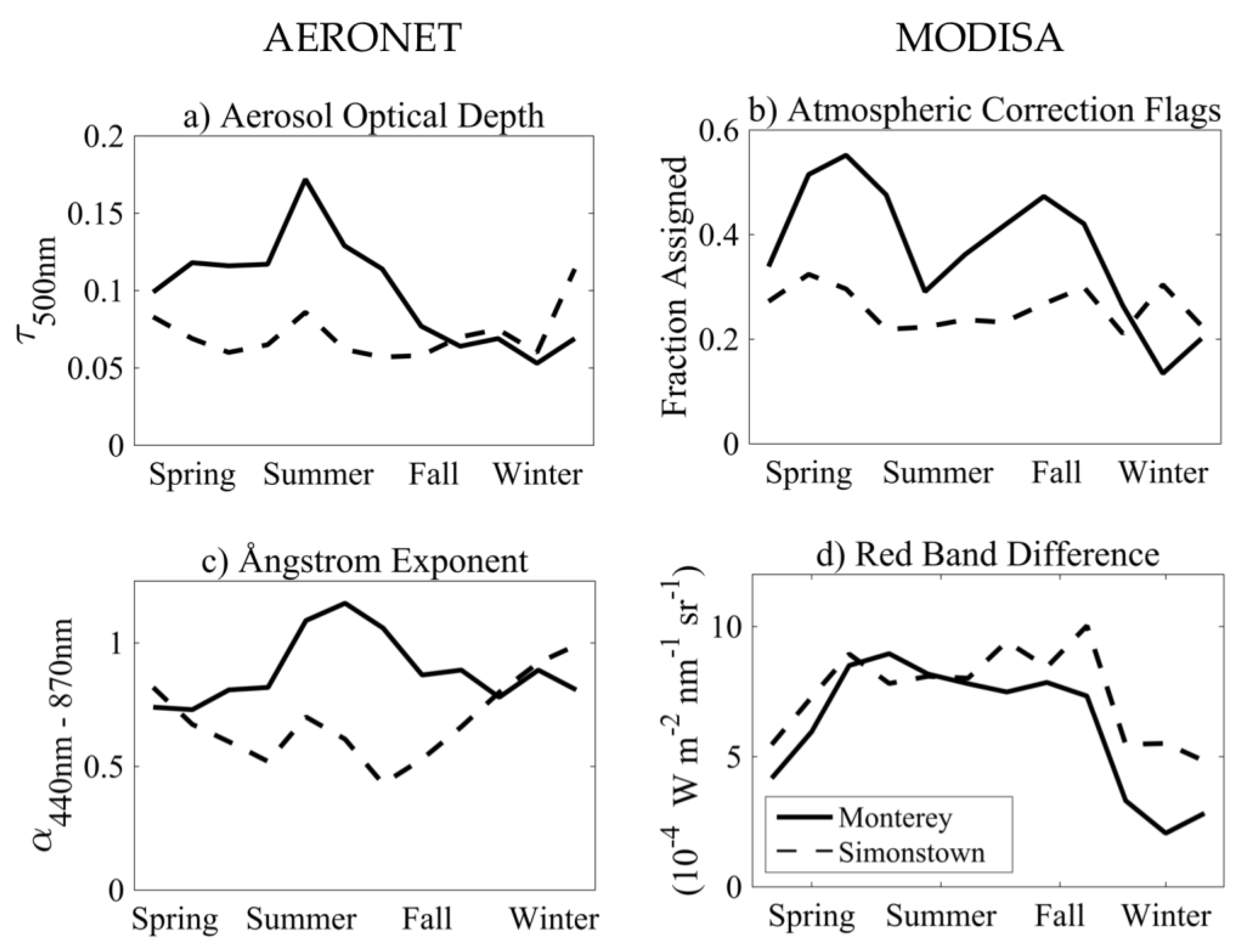
3.2. Climatology of Atmospheric Correction Flags

Comparison of AERONET and satellite (MODISA) climatologies did not reveal similarities between atmospheric constituents and satellite flags. In particular, results from a Pearson’s correlation test were not significant between AC flags and either aerosol optical depth (p = 0.25, p = 0.29) or Ångstrom exponent (p = 0.67, p = 0.84) for the Monterey or Simonstown sites, respectively. AC flag assignments correlated positively with RBD at both sites, with correlation significant for MB (p < 0.01) but not for SHB (p = 0.43). Both AERONET sites revealed local maxima of both aerosol optical depth and Ångstrom exponent during summer that did not correspond to a spike in AC flag assignments during the same month. For the Monterey site, the summertime peak in atmospheric complexity coincided in local minima in AC flag assignments suggesting that pollution or aerosol loading during summer months are not dominant mechanisms for low atmospheric correction efficacy in this sample. The seasonality of AC flags in the Simonstown region was more uniform than the Monterey region but was similarly incongruous with the AERONET results (Figure 3).

Although not elucidated by this analysis, the relatively higher Ångstrom exponent and aerosol optical depth measured from spring through fall at the Monterey AERONET station may in part be responsible for the decreased performance in the OC3M match-ups within MB compared with SHB. Other differences between the Monterey and Simonstown results may be due to the AERONET locations, with the Monterey site nearer the sheltered retentive zone in southern MB and the Simonstown site located near a headland with more exposure to wind and currents and further from the SHB subset.

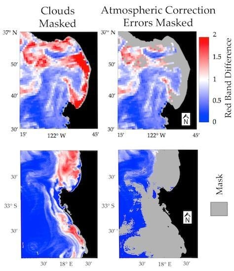
3.3. Impact of Atmospheric Correction Masks on Level 2 RBD datasets

Satellite retrievals with higher RBD values were more frequently assigned AC flags, with 33.8% and 33.1% of observations assigned AC flags within the upper quartile of RBD data and only 5.3% and 8.2% within the lower quartile at MB and SHB, respectively. As a result, masking of AC flagged retrievals decreased the right-hand tails of the RBD dataset distributions at both sites (Figure 4). The resultant masked fraction describes lower average RBD values (mean: −18.1% and −11.0%; median: −14.7% and −8.0%) with less variance (standard deviation: −13.3% and −13.0%) compared with the initial (AC flagged pixels not masked) datasets for MB and SHB, respectively.

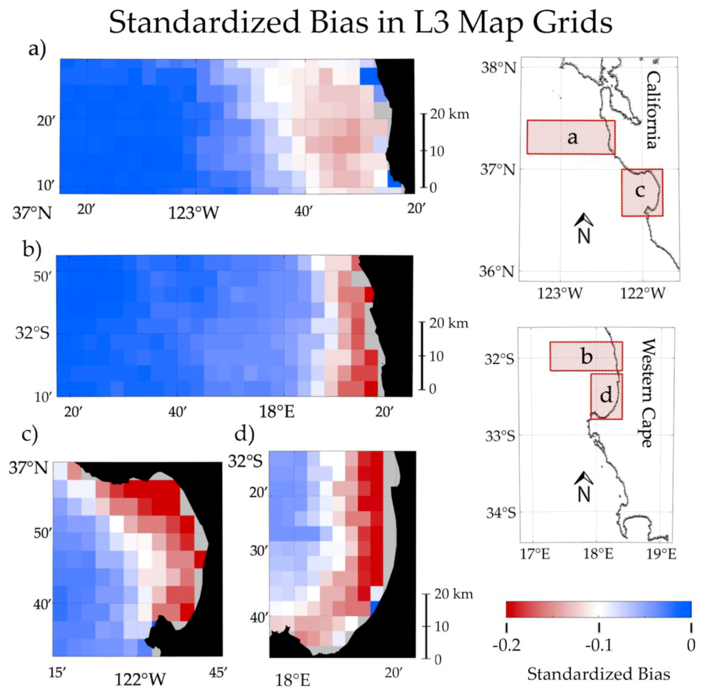
3.4. Impact of Atmospheric Correction Masks on Level 3 RBD Datasets

L3 spatial composites (4 km, 1 day) were compared between the masked and unmasked RBD datasets. Maximum negative SB occurred in the lee of retentive features that outline MB and SHB, regions prone to frequent phytoplankton blooms due to recirculation of water-masses and protection from offshore advection during upwelling pulses (Figure 5). SB was more negative in near-shore composite grids within the BCS compared with the CCS, with near-shore SB approximately a fifth of a standard deviation lower in the masked versus relaxed dataset. Amplitudes in SHB and MB were comparable, with SB of near-shore composite grids negative by approximately one quarter of a standard deviation.

Composites within the CCS and BCS transects (Figure 5a,b) were partitioned by longitude to derive SB as a function of distance from shore. Transect regions were adjacent to relatively north-south coastlines and were each greater than 50 km equatorward of the largest nearby coastline points (e.g., Point Reyes and Cape Columbine). The BCS transect showed more rapid improvement of data quality as a function of distance from shore, with SB less than a tenth of one standard deviation negative beyond approximately 30 km and 15 km within the CCS and BCS respectively (Figure 6). The greater offshore persistence of the negative SB for the CCS transect may be due in part to regional circulation differences such as proximity to upwelling hotspots and retentions zones. For example, high RBD amplitudes persist at all latitudes within the nearby SHB domain (Figure 5d), indicating that the BCS transect is in close proximity to a phytoplankton-rich, retentive zone. In comparison, the CCS transect lies poleward of MB and intersects a relatively unprotected stretch of coastline, favoring upwelling dynamics that generate offshore flow. Beyond approximately 50 km from shore, where phytoplankton concentrations are lower, both transects indicate convergence to a small SB, although the signs remain negative across our dataset.

From all four masked and unmasked L3 datasets, composites were partitioned by the fraction of AC flag assignments within each composite’s underlying (L2) pixels, which was recorded during L3 processing. The data products show near zero SB for composites with few AC flag assignments but the degradation in data quality increases for composites with greater fractions of L2 pixels masked by AC flags (Figure 7). The change in SB is strongly negative as the composites contain increasing pixels masked by AC flags, with the reduction approaching approximately four tenths of one standard deviation for heavily masked composites.

Despite the atmospheric, ecological and topographic differences between the BCS and CCS regions, the slope of the composite reduction is similar, implying consistency in the sites’ sensitivity to bias from the association between biology and retrieval quality. The slopes for all sites also imply a linear relationship due to the mixing of two distributions (masked and unmasked) within the composites. L3 transects used for this comparison include a broader range in water masses (onshore and offshore) and 4% of the composites in both the CCS and BCS contained a quarter or more L2 pixels assigned AC flags. Within the more productive regions of MB and SHB, 8% and 10% of the composites generated, respectively, contained a quarter or more L2 pixels assigned AC flags.

4. Discussion

4.1. Performance of Satellite Products at Match-up Sites

Based on the match-up results, RBD is a reasonable proxy to describe relative changes in Chla within the study regions, although this comparison is not intended as a validation activity to assess OC3M, C2RCC or other alternate processing methods. Indeed, for the OC3M products, atmospheric correction quality was a fundamental problem for the match-up regions but rigorous quality screening of the match-ups would have been counter to the goals targeted by this study, namely, to characterize the observations that fail such screenings. C2RCC performed marginally worse than RBD in the comparisons but it should be noted that although the C2RCC network is compatible with MODISA, development was not primarily targeted towards NASA products. Moreover, neural network algorithms require training sets representative of the regions assessed and our results are in no way intended to suggest that C2RCC would not outperform RBD under a different match-up set, or after addition of a larger training set. Indeed, in a recent intercomparison of atmospheric correction methods for coastal waters, strong improvements were shown for a C2RCC model after the inclusion of an expanded training set [22].

FLH algorithms such as RBD are useful for scene comparisons and as general Chla proxies but are not a satisfactory full solution to remote sensing challenges in coastal waters. Although Chla fluorescence and concentration generally covary, their relationship is inconsistent. Factors that may alter the relationship between Chla fluorescence and concentration include phytoplankton species composition, pigment packaging effects, physiology, limitation of nutrients or light or solar-induced fluorescence quenching [37]. The ability to measure fluorescence is also strongly affected by attenuation from water and its constituents, particularly by non-algal particles [38] and from sensor-specific response functions, for example, if the fluorescence peak shifts between response bands [39,40].

Despite the inherent difficulties in quantifying phytoplankton concentrations with Chla fluorescence products, such proxies are reasonable for the analysis shown here because of their relative robustness to atmospheric correction errors and because the RBD biomass comparison is not used across large spatial domains. Comparisons here are assumed to be relative within the region and as a result, this work did not focus on modeling RBD onto in situ Chla.

Products that use inputs from blue wavelengths (such as OC3M) were considered the most sensitive to the decrease in atmospheric correction efficacy addressed by the AC flag assignments and were not reasonable options for the comparison described here. Similarly, products such as OC3M often cannot be derived for AC flagged pixels, for example, when overestimation of aerosol thickness causes derivation of negative radiances at blue wavelengths. Finally, while RBD was preferred here over the OBPG default nFLH product because of its reported robustness to sediment effects, nFLH is expected to be a reasonable alternative for users who intend to perform a similar analysis of their study region but who require direct downloads of default L2 products.

4.2. Variability of Atmospheric Constituents and Efficacy of Ocean Color AC Flags

Atmospheric correction errors arising from elevated L_W(NIR) have been a focus for improving satellite retrievals over sediment- or phytoplankton-loaded waters. The associations shown here between AC flags and phytoplankton concentrations within MB and SHB are intended to demonstrate the frequency in which retrieval quality is linked to biology and to assess whether the set of observations which satisfy quality control thresholds are able to accurately characterize coastal marine ecosystems. In our study areas, the dataset fractions that satisfy default retrieval criteria (i.e., are not assigned AC flags) describe ecosystems which are generally reduced in biomass and have lower variability than described by the parent dataset. The results of this study, however, do not suggest that users relax AC flag criteria, because the flag assignments are in most cases reasonable indicators of degraded data quality, particularly in the portion of the spectrum relevant to blue-green band ratio algorithms (i.e., OC3M).

The removal of high biomass observations from the satellite record additionally screens out important biological processes, such as the formation of phytoplankton dense fronts and removes regions that may be disproportionately important to the ecosystem dynamics and species succession. For example, a northern MB retentive zone, which maintains dinoflagellate stocks that play an important role in species succession by seeding the surrounding waters [41], was frequently masked from the MB satellite record. We also note anecdotally that during red tide events within MB, ocean color retrievals on clear-sky days are often fully masked, with the satellite record resuming upon bloom termination.

4.3. Potential for User Evaluation of L2 and L3 Datasets

Defining the transition zone between regions where default NIR-based atmospheric correction methods can and cannot be used is challenging, as evidenced by the different transect results for the masked and unmasked composites for the two EBC ecosystems. The severity of the elevated L_W(NIR) effects may extend farther offshore than anticipated given the physics of the region (e.g., advection offshore by mesoscale eddies or jets). For regions where the removal of ephemeral high biomass events may be more infrequent, research targeting ecosystem processes may suffer from the loss of rare but high-impact events.

How can L2 and L3 end-users test whether satellite datasets contain a bias from the removal of high phytoplankton observations? L2 users with a priori knowledge of a region can compare flag assignments with expected phytoplankton dynamics to determine whether flags covary with target environmental parameters. For some flags, seasonality due to the Earth-sun geometry or cloud dynamics may resemble biological parameters without tracking phytoplankton biomass within an individual image. Interpretation of the flag assignment frequency should be considered cautiously, because infrequent flag assignments can have outsized effects in regions with high environmental variability. In the absence of a priori knowledge of a region, nFLH is anticipated to provide useful comparisons of the masked and unmasked data fractions, as shown herein. L3 end-users could make use of compositing statistics in order to assess the representativeness of spatial or temporal, quality-controlled averages. The similarity between sites in the relationship between composite SB and L2 flag assignments (Figure 7) suggests that L2 flag assignments are useful parameters for interpreting L3 composites. As such, metadata that includes flag assignment statistics may be a beneficial addition for disseminated L3 products, particularly for users requiring inputs for coastal ocean models.

5. Conclusions

Wide recognition of decreased performance of ocean color products in coastal waters has encouraged development of a variety of alternative methods aimed to overcome difficulties such as high organic and inorganic particle concentrations. However, no direct comparison of the masked versus unmasked fraction of satellite datasets or suggestions for determining a dataset’s sensitivity to the loss of high biomass retrievals, has been presented. This work compares non-aerosol-corrected biomass proxies to test whether high quality satellite retrievals are representative of initial datasets in coastal regions. Key findings shown are that, for productive ecosystems like MB and SHB, the changes to dataset distributions reflect a bias towards decreased biomass due to difficulty in removing the satellite signal’s atmospheric component over phytoplankton-rich waters. The changes in the biomass of L2 datasets are apparent in L3 composites and the distance that the changes extend offshore is variable even among broadly similar systems (i.e., EBCs). Finally, users may assess the sensitivity of their study site using a similar approach by comparing FLH products between the masked and unmasked fractions of their dataset or by deriving compositing statistics when generating L3 products. In cases where the masked fraction is dissimilar to the unmasked fraction, users may prefer to use alternative atmospheric correction methods regardless of the strength of validation results obtained from the masked fraction only. Research directed towards coastal ocean ecosystems should evaluate whether quality-controlled satellite estimates of phytoplankton concentrations are representative compared to the statistics of the parent dataset. When possible, TOA proxies are useful tools for such comparisons.

References

1. Gregg, W.W.; Conkright, M.E. Decadal changes in global ocean chlorophyll. Geophys. Res. Lett. 2002, 29, 1–4. [Google Scholar] [CrossRef]
2. McClain, C.R. A Decade of Satellite Ocean Color Observations. Annu. Rev. Mar. Sci. 2009, 1, 19–42. [Google Scholar] [CrossRef] [PubMed] [Green Version]
3. Dierssen, H.M. Perspectives on empirical approaches for ocean color remote sensing of chlorophyll in a changing climate. Proc. Natl. Acad. Sci. USA 2010, 107, 17073–17078. [Google Scholar] [CrossRef] [PubMed] [Green Version]
4. Siegel, D.A.; Wang, M.; Maritorena, S.; Robinson, W. Atmospheric correction of satellite imagery: The black pixel assumption. Appl. Opt. 2000, 39, 3582–3591. [Google Scholar] [CrossRef] [PubMed]
5. Sathyendranath, S.; Bukata, R.P.; Arnone, R.; Dowell, M.D.; Davis, C.O.; Babin, M.; Berthon, J.F.; Kopelevich, J.; Cmpbell, J.W. Color of Case 2 Waters. In Remote Sensing of Ocean Colour in Coastal and Other Optically-Complex, Waters; Sathyendranath, S., Ed.; Reports of the International Ocean-Color Coordinating Group: Dartmouth, NS, Canada, 2010; Volume 3, pp. 23–46. [Google Scholar]
6. Kahru, M.; Mitchell, B.G. Ocean color reveals increased blooms in various parts of the world. EOS Trans. Am. Geophys. Union 2008, 89, 170–172. [Google Scholar] [CrossRef]
7. Jessup, D.A.; Miller, M.A.; Ryan, J.P.; Nevins, H.M.; Kerkering, H.A.; Mekebri, A.; Crane, D.B.; Johnson, T.A.; Kudela, R.M. Mass stranding of marine birds caused by a surfactant-producing red tide. PLoS ONE 2009, 4, e4550. [Google Scholar] [CrossRef]
8. Lewitus, A.J.; Horner, R.A.; Carn, D.A.; Garcia-Mendoza, E.; Hickey, B.M.; Hunter, M.; Huppert, D.D.; Kudela, R.M.; Langlois, G.W.; Largier, J.L.; et al. Harmful algal blooms along the North American west coast region: History, trends, causes and impacts. Harmful Algae 2012, 19, 133–159. [Google Scholar] [CrossRef]
9. McCabe, R.M.; Hickey, B.M.; Kudela, R.M.; Lefebvre, K.A.; Adams, N.G.; Bill, B.D.; Gulland, F.M.D.; Thomson, R.E.; Cochlan, W.P.; Trainer, V.L. An unprecedented coastwide toxic algal bloom linked to anomalous ocean conditions. Geophys. Res. Lett. 2016, 43, 10366–10376. [Google Scholar] [CrossRef]
10. Pitcher, G.C.; Figueiras, F.G.; Kudela, R.M.; Moita, T.; Reguera, B.; Ruiz-Villareal, M. Key questions and recent research advances on harmful algal blooms in eastern boundary upwelling systems. In Global Ecology and Oceanography of Harmful Algal Blooms, 1st ed.; Gilbert, P.M., Berdalet, E., Burford, M.A., Pitcher, G.C., Zhou, M., Eds.; Springer: Cham, Switzerland, 2018; Volume 232, pp. 205–227. [Google Scholar]
11. Bracher, A.; Bouman, H.A.; Brewin, R.J.; Bricaud, A.; Brotas, V.; Ciotti, A.M.; Clementson, L.; Devred, E.; Di Cicco, A.; Dutkiewicz, S.; et al. Obtaining phytoplankton diversity from ocean color: A scientific roadmap for future development. Front. Mar. Sci. 2017, 4, 1–15. [Google Scholar] [CrossRef]
12. Frouin, R.J.; Franz, B.A.; Ibrahim, A.; Knobelspiesse, K.; Ahmad, Z.; Cairns, B.; Chowdhary, J.; Dierssen, H.M.; Tan, J.; Dubovik, O.; et al. Atmospheric correction of satellite ocean-color imagery during the PACE era. Front. Earth Sci. 2019, 7, 1–43. [Google Scholar] [CrossRef]
13. Barnes, R.A.; Clark, D.K.; Esaias, W.E.; Fargion, G.S.; Feldman, C.R.; McClain, C.R. Development of a consistent multi-sensor global ocean colour time series. Int. J. Remote Sens. 2003, 24, 4047–4064. [Google Scholar] [CrossRef]
14. Gregg, W.W.; Casey, N.W. Improving the consistency of ocean color data: A step toward climate data records. Geophys. Res. Lett. 2010, 37, 1–5. [Google Scholar] [CrossRef]
15. Kahru, M.; Kudela, R.M.; Manzano-Sarabia, M.; Mitchell, B.G. Trends in the surface chlorophyll of the California Current: Merging data from multiple ocean color satellites. Deep Sea Res. Part II Top. Stud. Oceanogr. 2012, 77, 89–98. [Google Scholar] [CrossRef]
16. Gordon, H.R.; Wang, M. Retrieval of water-leaving radiance and aerosol optical thickness over the oceans with SeaWiFS: A preliminary algorithm. Appl. Opt. 1994, 33, 443–452. [Google Scholar] [CrossRef] [PubMed]
17. Mobley, C.D.; Werdell, J.; Franz, B.; Ahmad, Z.; Bailey, S. Atmospheric correction for satellite ocean color radiometry. NASA Tech. Rep. Serv. 2016, 1, 1–85. [Google Scholar]
18. Wang, M.; Antoine, D.; Fruoin, R.; Gordon, H.R.; Fukushima, H.; Morel, A.; Nicolas, J.; Deschamps, P. Comparison Results. In Atmospheric Correction for Remotely-Sensed Ocean-Colour Products; Wang, A., Ed.; Reports of the International Ocean-Color Coordinating Group: Dartmouth, NS, Canada, 2010; Volume 10, pp. 23–38. [Google Scholar]
19. Wang, M. Remote sensing of the ocean contributions from ultraviolet to near-infrared using the shortwave infrared bands: Simulations. Appl. Opt. 2007, 46, 1535–1547. [Google Scholar] [CrossRef] [PubMed]
20. Ruddick, K.G.; Ovidio, F.; Rijkeboer, M. Atmospheric correction of SeaWiFS imagery for turbid coastal and inland waters. Appl. Opt. 2000, 39, 897–912. [Google Scholar] [CrossRef] [PubMed] [Green Version]
21. Brockmann, C.; Doerffer, R.; Peters, M.; Stelzer, K.; Embacher, S.; Ruescas, A. Evolution of the C2RCC neural network for Sentinel 2 and 3 for the retrieval of ocean colour products in normal and extreme optically complex waters. In Proceedings of the Living Planet Symposium, Prague, Czech Republic, 9–13 May 2016; Volume 740, p. 54. [Google Scholar]
22. Mograne, M.A.; Jamet, C.; Loisel, H.; Vantrepotte, V.; Mériaux, X.; Cauvin, A. Evaluation of five atmospheric correction algorithms over French optically-complex waters for the Sentinel-3A OLCI ocean color sensor. Remote Sens. 2019, 11, 668. [Google Scholar] [CrossRef]
23. Campbell, J.W.; Blaisdell, J.M.; Darzi, M. Level-3 Sea WiFS data products: Spatial and temporal binning algorithms. Oceano. Lit. Rev. 1996, 9, 952. [Google Scholar]
24. Scott, J.P.; Werdell, P.J. Comparing level-2 and level-3 satellite ocean color retrieval validation methodologies. Accepted Optics Express. 2019. [Google Scholar] [CrossRef]
25. Ryan, J.P.; Fischer, A.M.; Kudela, R.M.; Gower, J.F.R.; King, S.A.; Marin III, R.; Chavez, F.P. Influences of upwelling and downwelling winds on red tide bloom dynamics in Monterey Bay, California. Cont. Shelf Res. 2009, 29, 785–795. [Google Scholar] [CrossRef]
26. Pennington, J.T.; Chavez, F.P. Seasonal fluctuations of temperature, salinity, nitrate, chlorophyll and primary production at station H3/M1 over 1989-1996 in Monterey Bay, California. Deep Sea Res. Part II 2016, 47, 947–973. [Google Scholar] [CrossRef]
27. Pitcher, G.C.; Brown, P.C.; Mitchell-Innes, B.A. Spatio-temporal variability of phytoplankton in the southern Benguela upwelling system. S. Afr. J. Mar. Sci. 1992, 12, 439–456. [Google Scholar] [CrossRef]
28. Barlow, R.; Sessions, H.; Balarin, M.; Weeks, S.; Whittle, C.; Hutchings, L. Seasonal variation in phytoplankton in the southern Benguela: Pigment indices and ocean colour. Afr. J. Mar. Sci. 2005, 27, 275–287. [Google Scholar] [CrossRef]
29. Fawcett, A.; Pitcher, G.C.; Bernard, S.; Cembella, A.D.; Kudela, R.M. Contrasting wind patterns and toxigenic phytoplankton in the southern Benguela upwelling system. Mar. Ecol. Prog. Ser. 2007, 348, 19–31. [Google Scholar] [CrossRef] [Green Version]
30. Schumann, E.H.; Martin, J.A. Climatological aspects of the coastal wind field at Cape Town, Port Elizabeth and Durban. S. Afr. Geogr. J. 1991, 73, 48–51. [Google Scholar] [CrossRef]
31. Patt, F.S.; Barnes, R.A.; Eplee, R.E., Jr.; Franz, B.A.; Robinson, W.D.; Feldman, G.C.; Bailey, S.W.; Gales, J.; Werdell, P.J.; Wang, M.; et al. Algorithm updates for the fourth SeaWiFS Data Reprocessing. In SeaWiFS Postlaunch Technical Report Series; Hooker, S.B., Firestone, E.R., Eds.; NASA Technical Reports; NASA: Greenbelt, MD, USA, 2002; Volume 22, pp. 34–40. [Google Scholar]
32. Neville, R.A.; Gower, J.F.R. Passive remote sensing of phytoplankton via chlorophyll a fluorescence. J. Geophys. Res. 1977, 82, 3487–3493. [Google Scholar] [CrossRef]
33. Gordon, H.R. Diffuse reflectance of the ocean: The theory of its augmentation by chlorophyll a fluorescence at 685 nm. Appl. Opt. 1979, 18, 1161–1166. [Google Scholar] [CrossRef] [PubMed]
34. Letelier, R.M.; Abbott, M.R. An analysis of chlorophyll fluorescence algorithms for the Moderate Resolution Imaging Spectrometer (MODIS). Remote Sens. Environ. 1996, 58, 215–223. [Google Scholar] [CrossRef]
35. Gower, J.F.R. On the use of satellite-measured chlorophyll fluorescence for monitoring coastal waters. Int. J. Remote Sens. 2016, 37, 2077–2086. [Google Scholar] [CrossRef]
36. Amin, R.; Zhou, J.; Gilerson, A.; Gross, B.; Moshary, F.; Ahmed, S. Novel optical techniques for detecting and classifying toxic dinoflagellate Karenia brevis blooms using satellite imagery. Opt. Express 2009, 17, 9126–9144. [Google Scholar] [CrossRef] [PubMed]
37. Roesler, C.S.; Perry, M.J. In situ phytoplankton absorption, fluorescence emission and particulate backscattering spectra determined from reflectance. J. Geophys. Res. 1995, 100, 13279–13294. [Google Scholar] [CrossRef]
38. Gilerson, A.; Zhou, J.; Hlaing, S.; Ioannou, I.; Schalles, J.; Gross, B.; Moshary, F.; Ahmed, S. Fluorescence component in the reflectance spectra from coastal waters. Dependence on water composition. Opt. Express 2007, 15, 15702–15721. [Google Scholar] [CrossRef] [PubMed]
39. Gower, J.F.R.; Borstad, G.A. On the potential of MODIS and MERIS for imaging chlorophyll fluorescence from space. Int. J. Remote Sens. 2004, 25, 1459–1464. [Google Scholar] [CrossRef]
40. Ryan, J.P.; Davis, C.O.; Tufillaro, N.B.; Kudela, R.M.; Gao, B.C. Application of the Hyperspectral Imager for the Coastal Ocean to phytoplankton ecology studies in Monterey Bay, CA, USA. Remote Sens. 2014, 6, 1007–1025. [Google Scholar] [CrossRef]
41. Ryan, J.P.; Gower, J.F.R.; King, S.A.; Bissett, W.P.; Fischer, A.M.; Kudela, R.M.; Kolber, Z.; Mazzillo, F.; Rienecker, E.V.; Chavez, F.P. A coastal ocean extreme bloom incubator. Geophys. Res. Lett. 2008, 35, 1–5. [Google Scholar] [CrossRef]
Figure 1. MODIS Aqua imagery of phytoplankton blooms obtained on October 26th, 2016 in Monterey Bay, California (upper) and September 27th, 2011 near Cape Columbine, Western Cape (lower). (a) Pseudo-true color images with clouds masked in grey; (b) Red band difference (RBD) algorithm (a proxy for phytoplankton biomass) with clouds masked in grey; (c) RBD algorithm with clouds and suspect atmospheric correction (defined as maximum aerosol iterations reached and low water-leaving radiances) masked in grey.
Remotesensing 11 02167 g001
Figure 2. Location of biological and atmospheric measurements used in this study for (a) Monterey Bay, California and (b) St. Helena Bay, Western Cape. Chlorophyll-a and fluorometer measurement sites denoted with red circles, atmospheric measurement sites denoted with orange triangles. Regions of satellite L2 datasets used for analysis and matchups indicated by dashed black lines.
Remotesensing 11 02167 g002
Figure 3. Climatology of atmospheric and satellite products near Monterey Bay (MB) and SHB, shifted for the phase timing of northern and southern hemispheres (Monterey: solid black line, March–February; Simonstown: dashed black line, September–August): (a) Aerosol optical depth, (b) assignment frequency of AC flags (c) Ångstrom exponent and (d) Red Band Difference (RBD).
Remotesensing 11 02167 g003
Figure 4. Fraction of pixels assigned atmospheric correction (AC) flags as a function of RBD, with MB and SHB shown with solid and dashed black lines, respectively. The range shown encompasses greater than 98% of the data for both regions.
Remotesensing 11 02167 g004
Figure 5. Standardized bias in MODISA RBD composites (L3) due to the removal of underlying (L2) pixels, shown for standard map grids within the central California Current System (CCS) (a) and southern Benguela Current System (BCS) (b) and within MB (c) and SHB (d).
Remotesensing 11 02167 g005
Figure 6. Standardized bias in RBD composites (L3) across longitudinal transects due to the removal of underlying (L2) pixels assigned AC flags within the CCS (solid line) and BCS (dashed line).
Remotesensing 11 02167 g006
Figure 7. Standardized bias in RBD composites (L3) due to the removal of the underlying (L2) pixels assigned AC flags, as a function of L2 AC flag assignment, for L3 transects within the CCS (solid line) and BCS (dashed line) transects and within the MB (dashed-dotted) and SHB (dotted) composited regions.
Remotesensing 11 02167 g007