Intercomparison of Integrated Water Vapor Measurements at High Latitudes from Co-Located and Near-Located Instruments

Abstract

Data from global positioning system (GPS) ground-based receivers, ground-based microwave radiometers (MWRs), and radiosondes (RS) at two high-latitude sites were compared. At one site, the North Slope of Alaska (NSA), Barrow, Alaska (USA), the instruments were co-located, while at the other site, the second ARM Mobile Facility (AMF2), Hyytiälä, Finland, the GPS receiver was located about 20 km away from the MWRs and RS. Differences between the GPS-derived integrated water vapor (IWV) and the other three instruments were analyzed in terms of mean differences and standard deviation. A comparison of co-located and near-located independently calibrated instruments allowed us to isolate issues that may be specific to a single system and, to some extent, to isolate the effects of the distance between the GPS receiver and the remaining instruments. The results showed that at these two high-latitude sites, when the IWV was less than 15 kg/m², the GPS agreed with other instruments within 0.5–0.7 kg/m². When the variability of water vapor was higher, mostly in the summer months, the GPS agreed with other instruments within 0.8–1 kg/m². The total random uncertainty between the GPS and the other systems was of the order of 0.6–1 kg/m² and was the dominant effect when the IWV was higher than 15 kg/m².

1. Introduction

Although water vapor accounts for only about 0.25% of the total mass of the atmosphere, it determines most of the earth’s energy budget and large-scale circulation [1]. This critical and fundamental tropospheric component affects cloud distributions, storm initiation, and heat transport from the surface to upper layers, and it is therefore relevant for the thermodynamic properties of the entire atmosphere. Therefore, knowledge of the spatial and temporal distribution of water vapor is important for a variety of applications. Since about 1930, regular observations of moisture profiles have been possible thanks to the radiosonde (RS), and today a variety of instruments monitor water vapor at various temporal and spatial scales. Among these techniques, global positioning system (GPS) observations are of high relevance, and there has been a fast growth of ground network receivers (arranged into regional or global networks), making GPS crucial for water vapor monitoring. The estimate of integrated water vapor (IWV) from a GPS is possible thanks to the linear relationship between the zenith wet delay (ZWD) and the IWV present in the volume of atmosphere traversed by the signal from space to the ground receiver. Several studies conducted in various climatic regions of the earth have evidenced weaknesses and strengths of the GPS by comparing GPS measurements to measurements from RS, multichannel microwave radiometers (MWRs) [2,3,4], a very-long-baseline interferometry (VLBI) radio telescope [5], and numerical weather prediction models [6,7,8]. From a statistical point of view, intercomparison analyses have highlighted discrepancies in terms of systematic errors (bias) and random errors (standard deviation, SD). These discrepancies can be attributed to climatic conditions, the length of observations, and characteristics of the instruments such as instrumental errors, the volume sampled, sensitivity, and the sampling time as well as to water vapor retrieval algorithms.

The need to monitor and improve the quantification of water vapor is also essential considering incoming next-generation 5G wireless networks. In communications systems based on 5G technology, high data capacity and low latency are achieved by moving operational frequencies toward spectral regions such as the millimeter-wave band (30–300 GHz). From a communications point of view, for planning outdoor millimeter/submillimeter communication networks, water vapor is a source of signal degradations. To improve propagation models and experimental capability in the estimation of water vapor [9,10], accurate investigations of water vapor uncertainties in different climatic scenarios are desirable. However, even more importantly, since the critical 23.8-GHz water vapor frequency is so close to the 5G 24-GHz band, there is a high risk of interference, which impacts the ability to detect water vapor in the atmosphere accurately [11].

In this work, we specifically focus on IWV high-latitude observations, as their retrieval remains an important challenge in this climatic regime: for example, satellite retrievals suffer from high surface reflectivity and low solar zenith angle [12]. IWV from GPSes is often used as reference to evaluate critical satellite arctic retrievals [13,14,15], and its accuracy needs to be specifically quantified in this region. A recent IWV intercomparison analysis performed on data collected in St. Petersburg, Northern Russia (59°57′N, 30°42′E), based on MWR and RS data, showed SD and bias values ranging from 1.84 to 3.10 kg/m² and from 0.44 to 1.24 kg/m², respectively [16]. Similar studies conducted on data collected from high-latitude sites (located in Sweden, subarctic climate region) comparing the IWV from a GPS versus an RS showed an SD and bias of 0.66 kg/m² and 0.09 kg/m², respectively [17]. In a different study [18], the SD was equal to 1.23 kg/m², and the bias ranged from −0.35 to 0.34 kg/m².

We present the results of an IWV comparison performed on data collected at two high-latitude sites. The first site is in Hyytiälä (61°50′ N, 24°17′E), in the southern region of Finland. Data were collected during the Biogenic Aerosols–Effects on Clouds and Climate (BAECC) research campaign, conducted using the Atmospheric Radiation Measurement (ARM) Program’s second Mobile Facility, AMF2, in collaboration with the University of Helsinki in 2014. During the campaign, three co-located instruments (two MWRs and an RS) provided estimates of water vapor at the measurement site for almost one full year. These measurements were compared to data from a GPS receiver located in Orivesi, about 20 km from the ARM AMF2 site. The second site was in Barrow (71°19′ N, 156°36′ W), Alaska (USA), where the ARM program maintains a suite of tools for long-term climate monitoring. Co-located data from two microwave radiometers, a GPS, and radiosondes, collected during 2014, were analyzed. The purpose of this study was to provide an IWV intercomparison in the critical Arctic and subarctic region and to contribute to the understanding of the differences between observation systems by leveraging some of the differences in instrumentation between the BAECC and Barrow sites. The first unique feature was the presence of two co-located MWRs at both sites, which included a three-channel radiometer with an 89-GHz frequency and a 15-channel radiometer with frequencies near 183.3 GHz. Having two co-located, independently calibrated radiometers that provided measurements at different frequencies could help identify uncertainties in the calibration, as well as eventual drifts. On the other hand, the presence of three systems (two MWRs and a GPS) in addition to the RS could help to isolate issues associated with RS dry bias (e.g., Miloshevich et al. [19]). Lastly, the spatial distance between the GPS and the remaining instruments in Finland could provide some insights into the effect of the distance between the systems when compared to the Barrow co-located measurements.

The remainder of the paper is organized as follows: In Section 2 a description of the datasets is provided, and the methodology to extract water vapor from the measurements is explained. In Section 3, the results are presented. The different air volumes sampled by the sensors are discussed in Section 3.1, and in Section 3.2, a regression analysis between the instruments is performed providing statistical information on the overall agreement between the measurements. In Section 3.3, the bias and SD of the differences between the instruments are examined. In Section 4 and Section 5, a summary and conclusions are given.

2. Materials and Methods

In this section, we provide a brief overview of the measurement sites, datasets, and retrieval techniques applied to calculate the integrated water vapor (IWV) used in this work.

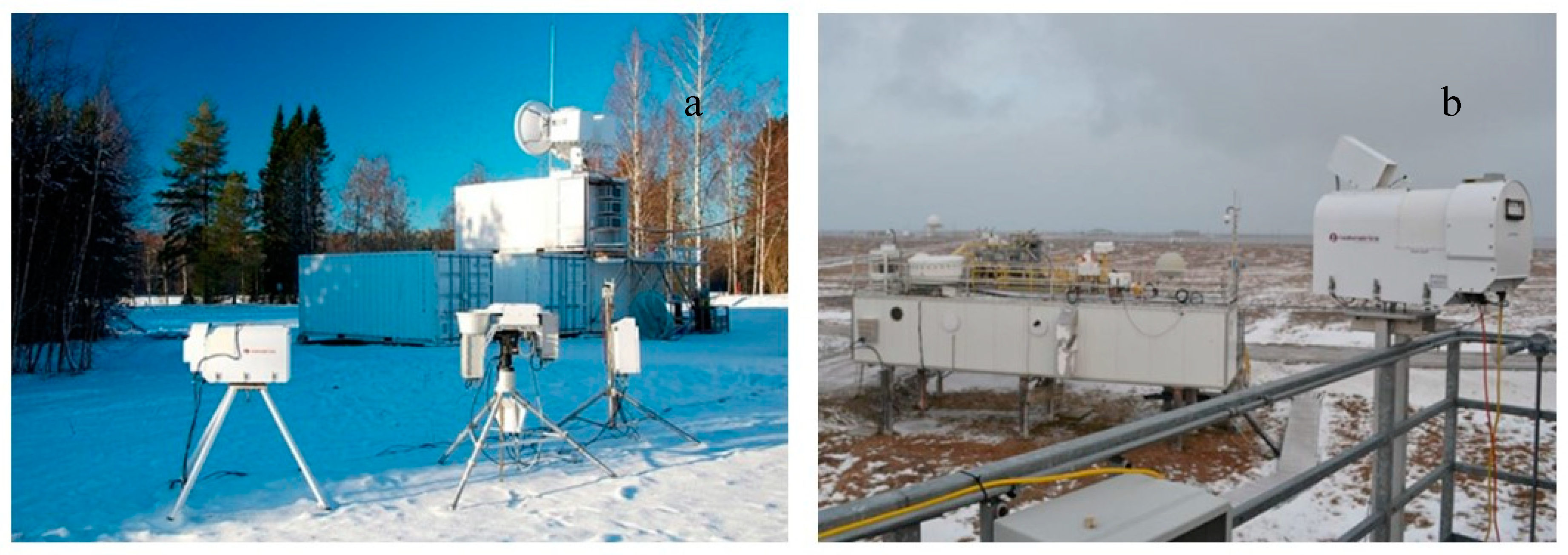
2.1. Microwave Radiometers and Radiosondes at the AMF2 Site

The ARM AMF2 deployment was installed in Hyytiälä, Finland, between January and September 2014, during the BAECC campaign [20]. Two MWRs were deployed as part of the ARM Program’s Mobile Facility (Figure 1, left panel). One radiometer (named 2C) operates at two frequencies, 23.8 and 31.4 GHz; the second (named 3C) has three channels at 23.834, 30.0, and 89.0 GHz. All K-band channels have a bandwidth of 300 MHz with a system noise temperature <500 K, and the 89-GHz channel has a bandwidth of 1900 MHz with a system noise temperature <1100 K. The integration time is 1 s for all radiometers. Although the two systems are fairly similar, there are some differences that are important for the present comparison. First, the two systems have different fields of view (FOVs): the 2C has a ~6° FOV (half-power beam width, HPBW) for both channels, and the 3C has a 3° FOV for all channels.

The time sampling is also different. The 2C samples have alternating faster zenith sampling (every 20 s) during cloudy conditions, with sampling every ~50 s during clear-sky conditions. The 3C collects zenith observations at 10-s intervals and performs tip scans at regular intervals of about 10 min. The most important difference, however, is the presence of the 89-GHz channel, which increases the 3C sensitivity to water vapor and cloud liquid water, making it a good instrument for locations at high latitudes. A detailed description of the radiometers and their calibration is given in the work of Cadeddu et al. [21]. Although the random uncertainty of the radiometric brightness temperature (B_T) is expected to be very low, on the order of 0.1 K, there are other factors that can affect the accuracy of long-term measurements. Drifts in the noise diode, as well as thermal effects on the radiometric components that are not thermally stabilized, can introduce seasonal and diurnal biases. This will be discussed in Section 3, where it will be shown that the inferior thermal stabilization of the 2C radiometer at the AMF2, compared to the north slope of Alaska (NSA), results in a temperature dependence of the mean differences between the 2C and the GPS. The 2C and 3C differ in their thermal stabilization and in how they handle the correction of residual temperature effects on the calibration. Additional biases can be introduced in the calculation of the opacity by the estimation of the mean radiating temperatures used in the tip calibration. The ARM radiometers are calibrated with a high degree of confidence and are expected to have a measurement root mean square error (RMSE) of around 0.3 K in the K-band and 0.5 K in the W-band (89 GHz). Based on the calibration accuracy and the sensitivity of each channel to water vapor, the nominal uncertainty in retrieved IWV from the two-channel radiometer is expected to be 0.5 kg/m²; however, with the addition of the higher frequency, it is possible to reduce the IWV uncertainty to about 0.4 kg/m² [22]. Although the ARM program provides routine retrievals of IWV and liquid water paths, statistical retrievals at the mobile facilities are less robust than those provided at the fixed sites (e.g., NSA) because the retrieval coefficients are usually derived using radiosondes launched during the campaign. For the BAEEC campaign, the RMSE for the IWV reported in the data files was ~0.80 kg/m² compared to 0.63 kg/m² reported for the NSA site. For this reason, a specific retrieval algorithm that uses 12 years of radiosonde data was developed for water vapor at the AMF2.

For this purpose, several regression algorithms were tested by using opacities τ(f_i) (in neper, Np) and brightness temperatures B_T(f_i) (in degrees kelvin) at the sampled operative MWR channel frequencies (f_i) as predictors. The algorithms use various polynomial combinations of the predictors, and different computations of the mean radiating temperature as a function of surface parameters [2,23,24] were investigated to calculate the predictor τ(f_i). Retrieval coefficients were derived using a long-term RS database collected in Jyväskylä (Finland), and the performances of the selected algorithms were compared. The Jyväskylä database encompasses 12 years (2003–2014) of RS profiles about 90 km away from the ARM AMF2 site. Based on data from the National Aeronautics and Space Administration (NASA) Advanced Spaceborne Thermal Emission and Reflection Radiometer (ASTER) Global Digital Elevation Model (GDEM), which has an estimated accuracy of ~15 m, the two sites are at the same elevation within 10 m, and therefore no corrections were applied to the radiosonde in the database. All simulations were carried out by applying the radiative transfer equation, together with a cloud model, to the RS database [25,26]. In this way, the retrieval coefficients accounted for the sensitivity to liquid water of all three channels. The retrieval algorithm based on a linear combination of B_T(f_i) was found to give the best agreement with the RS IWV in the testing subset of profiles, with a relatively small SD of 0.72 kg/m² and a correlation coefficient of 0.997. This algorithm, based on brightness temperature (Equation (1)), was therefore chosen to retrieve IWV from the AMF2 site measurements used in the next section:

$$\mathrm{IWV}={\mathrm{a}}_0+{{\displaystyle \sum }}_{\mathrm{i}=1}^{\mathrm{n}}{\mathrm{b}}_{\mathrm{i}}{\mathrm{B}}_{\mathrm{T}}\left({\mathrm{f}}_{\mathrm{i}}\right),$$

(1)

where n is the number of radiometric frequency channels (n = 3 for the 3C and n = 2 for the 2C), and a₀, b_j represent the computed linear inversion coefficients. The linear relationship of IWV to B_T holds for the very low B_T temperatures corresponding to the low IWV values found in the Arctic. As IWV increases, linearity holds with atmospheric opacities [24]. Although the radiometer retrievals are trained using a large radiosonde database, they are independent from the radiosondes because of the high sensitivity of the radiometer itself to the IWV. Radiometric calibration is the main factor that can affect the accuracy of the retrieved IWV.

During the BAECC research campaign, atmospheric profiles were collected by RS, Vaisala Model RS92, four times per day (at 05:00, 11:00, 17:00, and 23:00 UTC) near the MWR stations. The performance of the RS92 humidity sensor has been the subject of several investigations [19,27,28]. In particular, Wang and Zhang [27] have observed that RS92 profiles can be affected by solar radiation dry bias (dependent on pressure, season, and time of day), which requires a relative humidity correction. RS dry bias has been extensively documented, e.g., by Miloshevich [19], who estimated a precision of about 5% for the RS-derived IWV; and by Cady-Pereira et al. [28], who proposed a correction dependent on the solar zenith angle. More recently, Wang et al. [29] proposed corrections of the order of 2% to 4% in the lower mid-troposphere and 6% to 8% in the upper troposphere. The radiosonde data used in this study were downloaded from the ARM Archive. The data were processed using the Vaisala-provided algorithm. The vertical resolution of the profile is 10 m, and the profiles usually end at a height of 20–25 km. ARM data are quality-controlled, as explained in Peppler et al. [30,31], and quality control flags are applied to the data. Finally, a dry bias correction was applied to the RS data, as discussed in Section 3.3.

2.2. GPS-Derived IWV Data

The Zenith Total Delay (ZTD) by the neutral atmosphere, can be expressed as the sum of two components: zenith hydrostatic delay (ZHD) due to hydrostatic gases (mainly oxygen) and zenith wet delay (ZWD) due to water vapor. In this work, ZTD is used to derive ZWD, which is, in turn, related to the atmospheric IWV according to Equation (2):

$$ZWD=ZTD-ZHD.$$

(2)

The ZHD used in Equation (2) can be accurately modeled from knowledge of the total surface air pressure, latitude, and altitude of the GPS ground-receiver station above the geoid [32,33]. The error introduced by assuming hydrostatic equilibrium is typically of the order of 0.01%, which corresponds to a submillimeter accuracy in the zenith delay. Nevertheless, under extreme conditions, it can amount to several millimeters [4]. The uncertainty in the calculation of ZHD is mainly due to uncertainty in surface pressure, the refractive constant, and the dry gas constant [33]. An error in the surface pressure of 1 hPa will lead to a 2.3-mm error in the ZHD and about 0.35 kg/m² in the IWV [34]. Because a pressure sensor is not available at the GPS site, the ZHD was computed using the air pressure provided by a meteorological ground station located at the AMF2 site. Based on ASTER GDEM data, the difference in elevation between Orivesi and AMF2 at Hyytiälä is less than 10 m. This broadly results in a pressure difference of ~1 hPa. Assuming that the wet path delay is entirely due to the amount of water vapor traversed by the signal, the IWV can be computed from the ZWD via a dimensionless conversion factor π (see, e.g., Reference [35]), as shown in Equation (3):

$$IWV=\pi \ast ZWD.$$

(3)

As can be seen from Equations (2) and (3), uncertainties in GPS-derived IWV arise from uncertainties in ZTD processing as well as uncertainties in π and ZHD. Ning et al. [18,34] assessed that, because the ZHD can be estimated fairly accurately, ZTD processing contributes about 75% to the total IWV uncertainty. The dimensionless factor π is a function of various physical constants and of the weighted mean atmospheric temperature (T_m) [35]. T_m is commonly computed from surface air temperature using a linear regression [36] with an RMSE of 2–5 K. T_m is generally site-dependent and varies seasonally and diurnally [35]. An alternative approach for estimating π consists of deriving a linear regression between IWV and ZWD, making use of a historical database of radio soundings from which both parameters can be computed [36]. Applying this approach, monthly averages of π were calculated for use in Equation (3). The large RS database collected in Jyväskylä that was used to derive the radiometric coefficients (as described in Section 2.1) was also used to compute the ZWD and IWV associated with each profile. As expected, the calculated π displayed a seasonal variability, with a maximum value in July (0.158) and a minimum value in February (0.148). In order to evaluate the impact of the conversion factor π on the uncertainty of GPS IWV, the contribution of π to the IWV uncertainty is evaluated as

$${\sigma }_{IWV}={\sigma }_{\pi }\ast \overline{ZWD},$$

(4)

where ${\sigma }_{\pi }$ is the monthly calculated SD of the conversion factor, and $\overline{ZWD}$ is the monthly averaged $ZWD$. To express this uncertainty as a percent, ${\sigma }_{IWV}$ can be divided by the monthly mean IWV. The resulting IWV uncertainty varied from 1.15% (July) to 1.83% (February) and was lower than the 2.8% error obtained when using a single annual value, as shown in

Table 1. Statistical uncertainty of the global positioning system (GPS)-derived integrated water vapor (IWV) due to the conversion factor (π) expressed as a percent of the average monthly water vapor content.

Month	π	$\mathbf{Uncertainty},{\mathbf{\sigma }}_{\mathbf{I}\mathbf{W}\mathbf{V}}[\%]$	$\overline{\mathit{I}\mathit{W}\mathit{V}}(\mathbf{kg}/{\mathbf{m}}^2)$
1	0.148	1.74	5.94
2	0.148	1.83	5.24
3	0.149	1.80	5.88
4	0.151	1.44	8.03
5	0.154	1.68	12.45
6	0.156	1.44	15.74
7	0.158	1.15	23.20
8	0.157	1.26	20.42
9	0.155	1.26	15.35
10	0.153	1.54	11.21
11	0.151	1.62	8.75
12	0.149	1.67	7.29
All year	0.152	2.77	12.28

.

The use of monthly values leads to a reduction in the IWV uncertainty of between 34% and 58%, depending on the month. This method seems to fit well the climatic conditions of the investigated observations, introducing low relative errors in the GPS-derived IWV [36]. All of the uncertainties mentioned above, with additional factors due to multipath effects [37], contribute to the total uncertainty of the GPS-derived IWV. As mentioned earlier, at the AMF2 site, the GPS ground-based receiver was located 20 km away from the other instruments. The GPS data were obtained by the Finnish Geodetic Institute and the National Land Survey of Finland as Receiver INdependent EXchange format (RINEX) files and processed in Precise Point Positioning [38] mode using the Global Navigation Satellite System (GNSS)-Inferred Positioning System and Orbit Analysis Simulation Software package GIPSY-OASIS II [39], with a cut-off angle of 3°. We fixed Jet Propulsion Laboratory (JPL) fiducial-free satellite orbits, clocks, and earth orientation parameters and state-of-the-art processing options to estimate ZTD with a 5-min sampling [40,41]. The Vienna mapping function [42] was applied to the delay of the signal along each satellite-receiver path in order to map it into the zenith direction.

2.3. Instrumentation at the North Slope of Alaska

The ARM Program maintains a suite of instruments at the north slope of Alaska (NSA) site, located in Barrow, Alaska [43]. In this work, data from two MWRs, a GPS, and an RS, collected in 2014, were used (Figure 1, right panel). The first microwave radiometer was a 2-channel system (2C) identical to the one described in Section 2.1. ARM NSA IWV routine retrievals from the 2C are derived from atmospheric opacities as predictors in a linear regression. The second radiometer was the G-band vapor radiometer profiler (GVRP), which has 15 channels between 170 and 183.3 GHz and is suited for the retrieval of small amounts of water vapor. Because the frequencies saturate quickly as the IWV increases, the range of operability of the radiometer is restricted to IWV < 10 kg/m². The optimal IWV for the GVRP operation is below 6 kg/m². The IWV from the GVRP is retrieved using a neural network algorithm, as described in Reference [44]. Radiosondes are launched at the NSA site twice per day (05:00, 17:00 UTC) and are of the same type used at the AMF2 site. Finally, the GPS data at the NSA are part of the Suomi GPS network [45] and were downloaded from the ARM Archive as part of the Global Earth Coverage data stream. The IWV is provided along with the delay information. The conversion factor π at the NSA is derived at each point using the mean atmospheric temperature from the National Centers for Environmental Prediction (NCEP) Global Forecast System (GFS) model. The data are processed using the Bernese 5.0 software with a cut-off angle of 3° and are provided with a temporal resolution of 30 min. Pacione et al. [41] evaluated the agreement between the different GPS software packages—Bernese [46], GAMIT [47], and GIPSY-OASIS II [39]—in terms of the ZTD standard deviation. They found that the overall agreement is better than 3 mm before 26 March 2000 and 2 mm thereafter. This translates to water vapor agreement of about 0.3–0.5 kg/m².

3. Results

The IWV derived from the four deployed systems (the GPS, two MWRs, and RS) at the two sites is analyzed in this section. Since each system has its own intrinsic uncertainties, differences between measurements will also depend on different temporal sampling and spatial fields of view. At the AMF2, the GPS is located about 20 km away from the MWRs; the RS are launched at both sites but quickly drift away; and the two radiometers sample in zenith view with different FOVs. This aspect of the comparison, related to the different volumes sampled by the instruments, is examined in detail in Section 3.1. Measurement agreement is analyzed by examining the mean value of the differences (mean difference) and their standard deviation, as shown in Section 3.2. Further information is provided by regression analysis, i.e., by examining the correlation between the measurements throughout the campaigns. A regression analysis can help in the identification of biases or dependencies of the differences in factors such as water vapor amount or temperature.

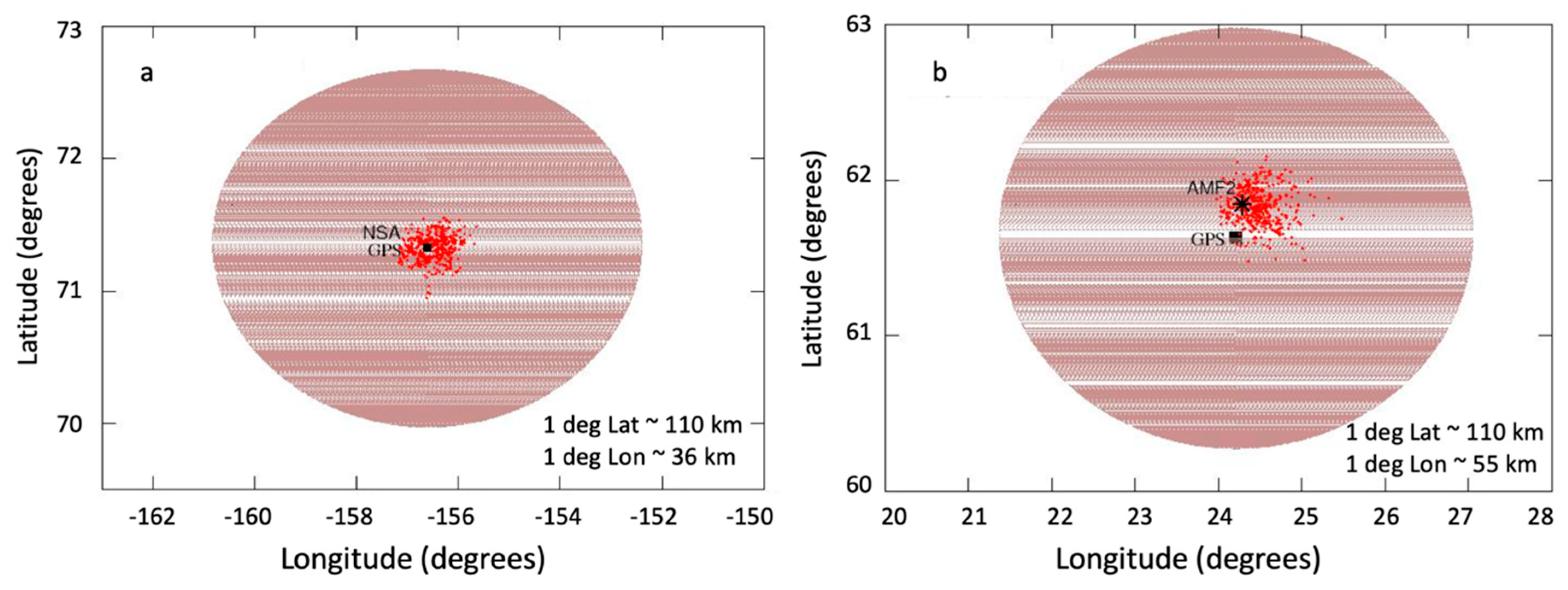
3.1. Instrument Field of View

Table 2. Characteristics of the IWV uncertainty instruments used in the analysis. RS: radiosonde; FOV: field of view; HPBW: half-power beam width.

Parameter	GPS	3C	2C	GVRP	RSAMF2	RSNSA
FOV (°, HPBW)	174	3.50	6.50	1.8	-	-
Area radius 1 (km)	153	0.25	0.45	0.837	17.4 1	13.8 2
Nominal instrument uncertainty (kg/m2)	0.6	0.4	0.5	0.4	0.2	0.2
Reference	[34]	[21]	[21]	[21]	(See text)	(See text)

¹ Radius of the base of the FOV cone at 8-km height; ² average drift at 8-km height.

summarizes the characteristics of the instruments operated in both sites, as discussed in Section 2. The GPS, with its large field-of-view, samples a broad portion of the sky from horizon to horizon, averaging the water vapor through a large volume. Conversely, the radiometers strictly sample the water vapor above the observation site. The radiometers and the GPS provide measurements of water vapor in the troposphere at temporal resolutions of 10 s and 5 min, respectively, at the AMF2 (30 min for the GPS at the NSA), whereas radiosondes can be subjected to wind gradients that can strongly change the ascension speed of the probe. At the latitude considered in this work, the average tropopause height above which water vapor becomes negligible is about 8 km [48]. During the BAEEC campaign, when the radiosondes reached 8 km in height, they had drifted on average 17.5 km. The GPS and radiometers sample a volume enclosed in a viewing cone with its vertex located at the instruments’ location. The radius of the base of the cone at 8 km of height is provided in the first row of Table 2 for each remote sensor. Note that GPS data are processed with a 3° cut-off angle at both sites. The third row of Table 2 reports the nominal uncertainty of each instrument. To estimate the uncertainty in the RS-integrated water vapor, a random perturbation of 0.5 K was applied to each layer of the temperature profiles, and 5% perturbation was applied to each layer of the humidity profiles. The resulting IWV was computed for the entire AMF2 dataset, and the distribution of the differences between unperturbed and perturbed IWV never exceeded 0.2 kg/m². Figure 2 shows the location of the radiometers (star) and GPS (square) sites and the location of all radiosondes launched during the campaign when they reached 8 km in height. The shaded ellipse represents the area covered by the GPS FOV at the same height.

From Figure 2, it is evident that at AMF2, when the radiosondes reached 8 km in height, they were clustered in an area approximately 20 km away from the launch site; however, there were several radiosondes that drifted farther away, covering an area of ~40 km. Although both the radiometers and the majority of the radiosondes were included in the GPS field of view, a large portion of the volume sampled by the GPS was entirely out of the radiosonde coverage area. Differences between the GPS and radiometer/radiosonde water vapor measurements were partially due to the variability of the water vapor in each instrument’s FOV and partially due to the fact that the GPS and the radiometers/radiosondes were sampling different air masses. On the other hand, the radiosondes at the NSA, Barrow, site had less spatial variability and were clustered around the center of the GPS field of view. The variability between the measurements was affected by the FOV of the instruments; however, at the AMF2, the effect of the distance between the GPS and the radiometers compounded the intrinsic effect of the FOV.

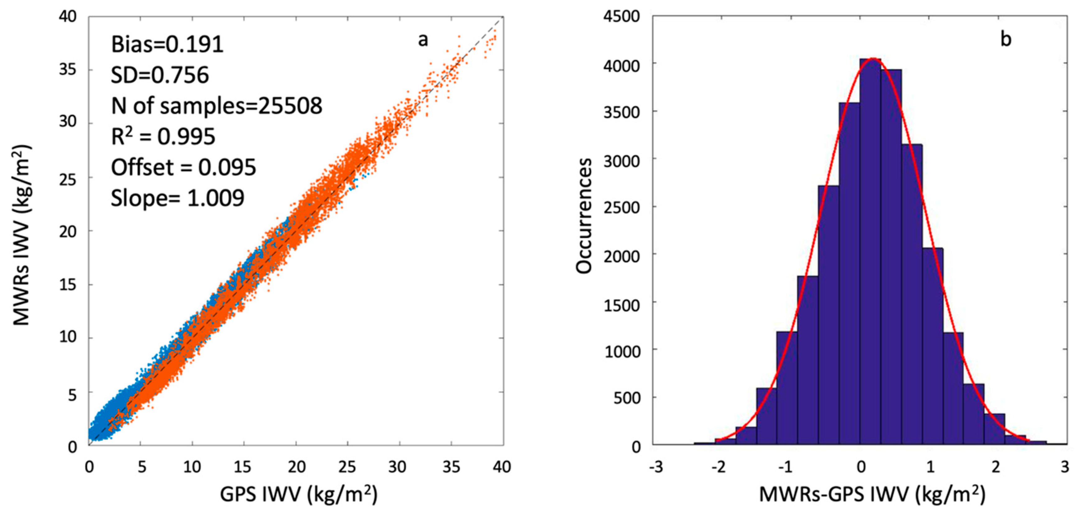
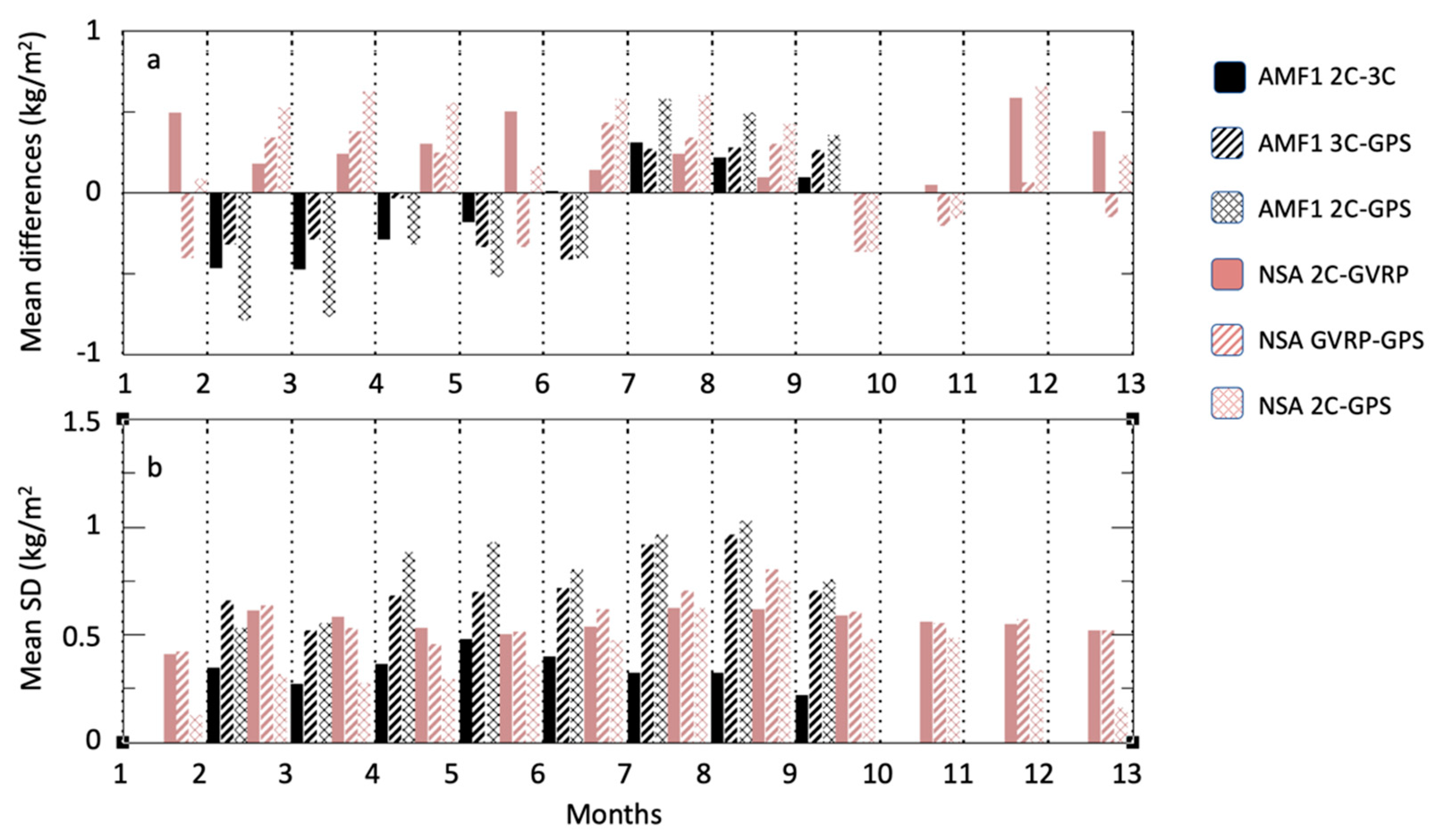
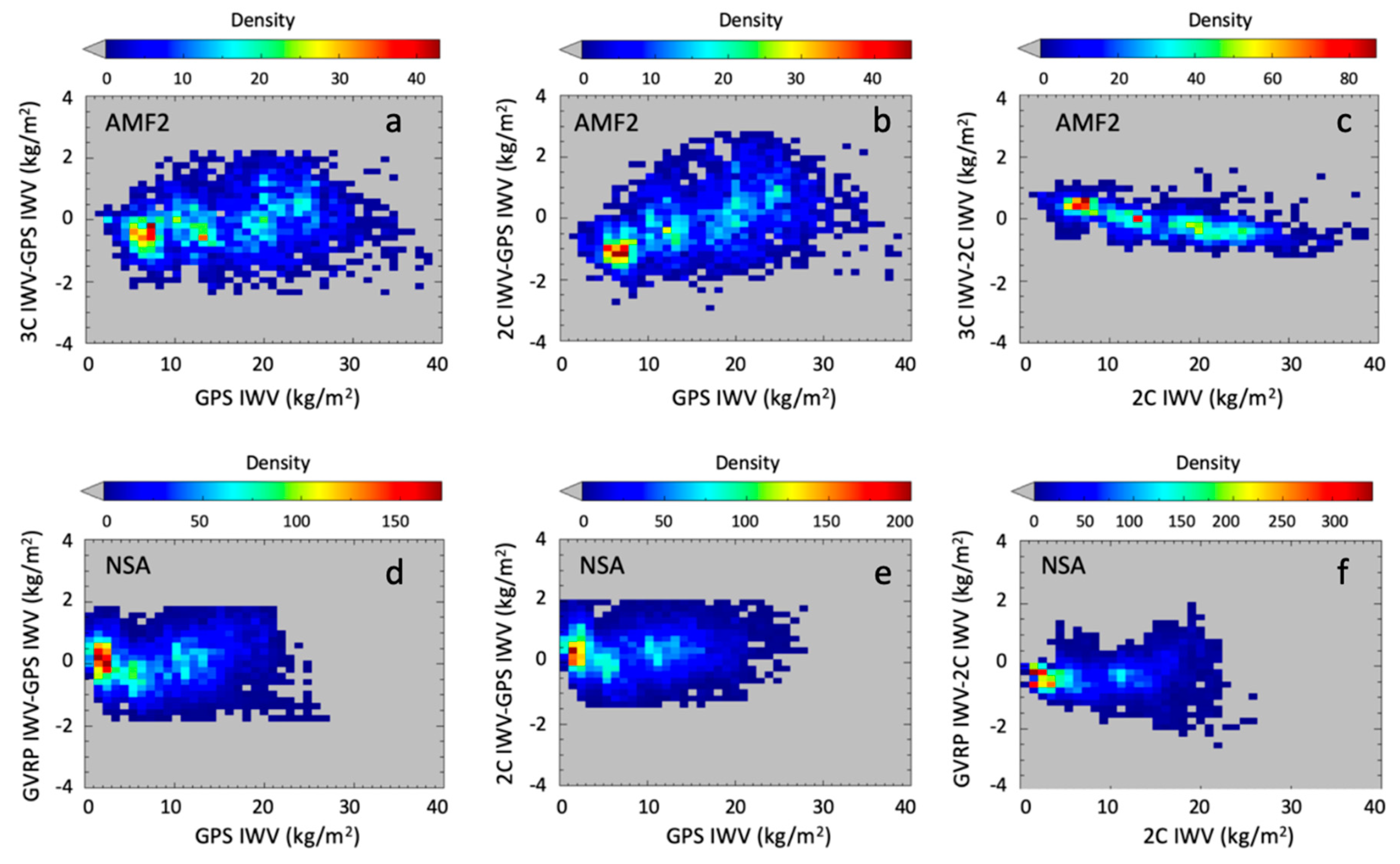
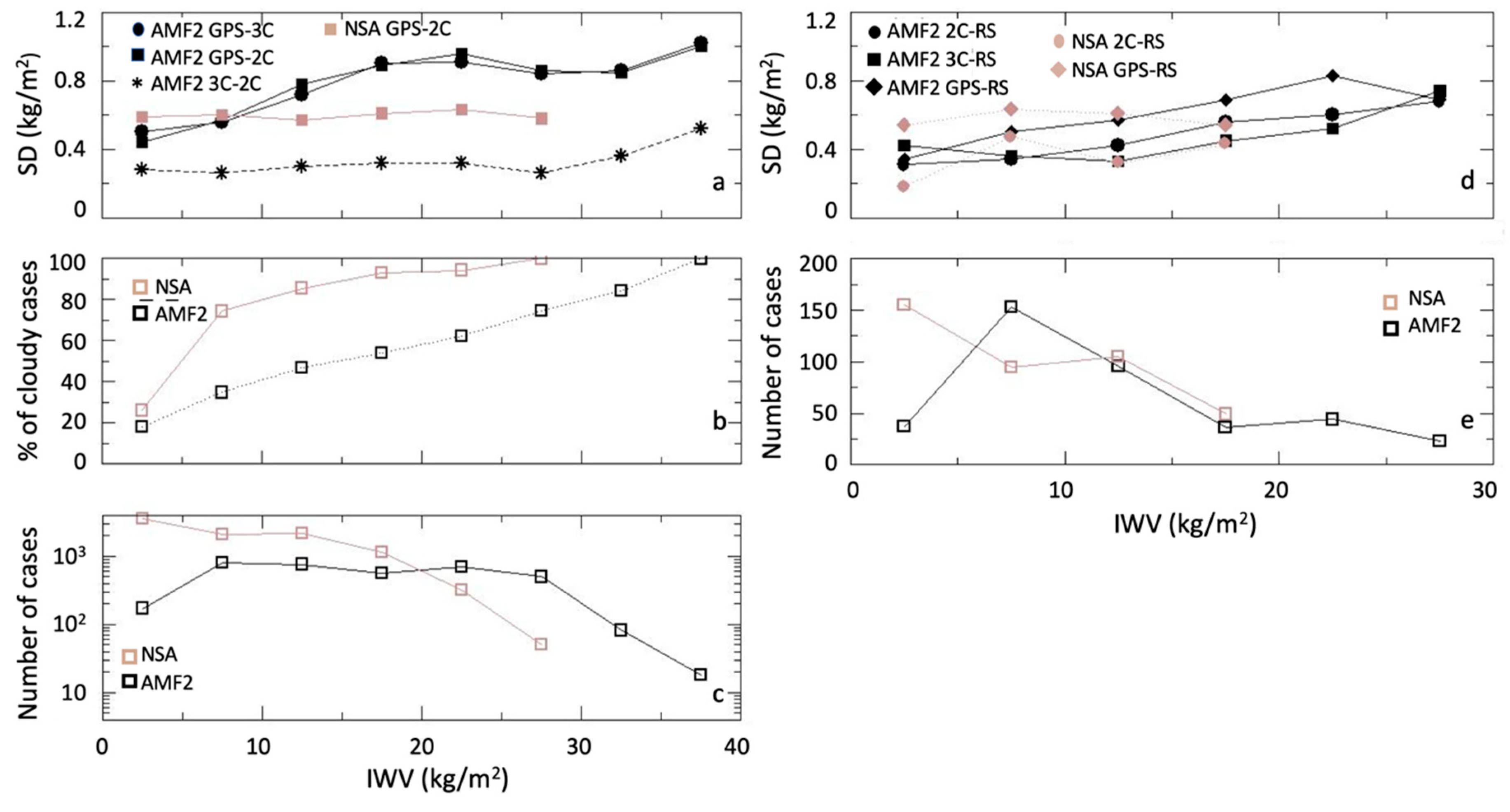
3.2. Analysis of 30-Min GPS Radiometer Data at the Two Sites

The IWV derived at the two sites was averaged over 30 min, and outliers were eliminated using an interquartile threshold. Most of the outliers were caused by residual water contamination on the radiometers after rain or snow. These were identified computing the 25th and 75th percentile, and the points that were 1.5 times outside this interquartile range were eliminated. At the NSA site, the IWV observations amounted to 9195 concurrent and co-located samples between January and December 2014. At the AMF2, there were 3604 concurrent (but not co-located) measurements from February to September 2014.

When examining together the IWV from AMF2 and NSA, comparing all radiometers versus the GPS, an excellent agreement (bias = 0.191 kg/m², SD = 0.756 kg/m², and R² = 0.995) was found, as shown in Figure 3a. From that, an overall data consistency could be determined. The offset and slope had values of 0.095 kg/m² and 1.009 kg/m², respectively. The distribution of the differences is shown in Figure 3b together with a fit to a normal distribution (red solid line). That latter plot shows that the IWV differences were normally distributed. A more detailed analysis of the two datasets, however, showed subtle differences between the two sites that were due to the different regional features of the water vapor patterns and that may be important when trying to evaluate the regional performance of the instruments. At NSA, extremely dry conditions commonly occur during the winter months, with the IWV often less than 3 mm [22]. In our dataset, the IWV ranged from a minimum value (min) of 0.68 kg/m² to a maximum value (max) of 27.53 kg/m², with an annual average of 8.39 kg/m². At AMF2, more humidity is present, with a min of 2.15 kg/m², a max of 38.07 kg/m², and an average of 16.21 kg/m².

Table 3. Statistical parameters of the IWV intercomparisons for the 30-min data (units are kg/m²). N is the number of points used at each site.

AMF2 (N = 3604)				NSA (N = 9195)
	3C versus GPS	2C versus GPS	3C versus 2C	GVRP versus GPS	2C versus GPS	GVRP versus 2C
Bias	−0.016	0.029	0.013	0.140	0.408	−0.268
SD	0.837	1.013	0.441	0.677	0.610	0.492
Slope	1.028	1.069	0.961	1.014	1.003	1.009
Offset	−0.471	−1.148	0.649	0.026	0.385	−0.341
R2	0.995	0.994	0.999	0.993	0.994	0.996

reports the bias, SD, correlation coefficients (R²), and regression parameters of the GPS radiometer comparison for both sites. At the NSA, the agreement between the independent co-located estimates was very good throughout the IWV range, as shown in Figure 3a. The comparison between the GVRP and GPS displayed increased random variability (SD ~ 0.68 kg/m²) with respect to the other comparisons at the same location. However, the bias and offset (0.140 kg/m², 0.026 kg/m²) were the smallest, and the dispersion was uniform throughout the IWV range. The higher frequencies near 183.3 GHz enhanced the sensitivity of the instrument for small amounts of water vapor; however, they also limited its operating range to IWV < ~10 kg/m², and therefore, retrievals above this threshold were less accurate and showed higher variability. The comparison between the 2C and GPS showed a bias of 0.408 kg/m² and a slope of 1.003 kg/m². The 2C IWV seemed to be slightly higher than the GPS IWV (and the GVRP IWP), but on the other hand, the SD of ~0.61 kg/m² was slightly better than in the case of the GVRP. Besides the bias difference, the two radiometers (GVRP and 2C) showed overall good agreement with the slope of 1.009, R² values of 0.996, and an SD of 0.492 kg/m². The observed random variability of the differences was within the expected random variability of the instruments and in particular of the GPS. The small offsets between the instruments were also in the expected systematic uncertainty of the systems, which was in the order of 0.4–0.5 kg/m² (see Table 2).

At AMF2, the 3C had the best agreement with the GPS, with almost no bias (~-0.016 kg/m²), an SD of ~0.837 kg/m², and a slope of 1.028. The intercomparison between the IWV from the 2C and the GPS showed a slight bias and an SD of 0.029 and 1.013 kg/m², respectively. The two radiometers had very low bias (0.013 kg/m²) and the lowest random variability (SD = 0.441 kg/m²) with the best R² value (0.999). It was noticeable that the bias at the AMF2 was much smaller than at the NSA. The reason for this behavior can be seen in Figure 3a, where IWV values from all radiometers are compared to the GPS IWV for a total of 25,598 samples. With respect to the GPS, the AMF2 radiometers (orange points) slightly underestimated the IWV below ~20 kg/ m² and overestimated at higher amounts, compensating for the bias when the entire dataset was considered. This is also visible in Figure 4, which shows the monthly mean differences (top) and their standard deviations (bottom) at the NSA (brown) and AMF2 (black) sites.

The NSA mean differences showed little seasonal dependence, with biases generally less than 0.6 kg/m² and an SD of comparable magnitude. The AMF2 mean differences, on the other hand, displayed a seasonal dependence, in particular in the comparison between the GPS and 2C, although a small dependence was also seen between 3C and GPS. A consistent feature of the comparison was the fact that the SD between the GPS and the radiometers (dashed and crossed black bars in the bottom panel) was higher compared to the SD between the radiometers. This was due to the larger FOV of the GPS and, at the AMF2 site, to the distance between the GPS and the other sensors. Moreover, the SD between the GPS and radiometers increased during the summer months. A similar behavior was observed by Haase et al. [49] and was attributed to increased water vapor inhomogeneity during the summer months. A clearer picture could be gained by plotting the mean differences as a function of IWV, as shown in the density plots of Figure 5. The 2C mean differences with respect to the GPS at the AMF2 appeared to have a dependence on IWV that was not present at the NSA. This led to a slight underestimation of the IWV when the IWV was <15 kg/m² and to an overestimation when the IWV >15 kg/m², leading to a higher intercept and lower slope than in the other two systems (GPS and 3C). This behavior was not observed in the NSA 2C (Figure 5b,e), although the two instruments were similarly calibrated. One possible explanation could be the additional thermal insulation provided to the NSA 2C, which was designed to stabilize the noise diode and mixer for Arctic operations. The AMF2 radiometer is not equipped with the additional insulation. Another possible explanation for this behavior is the difference in the retrieval algorithms used at the two sites. As previously mentioned, the AMF2 retrievals were based on a polynomial fit to the brightness temperature, while the NSA retrieval was based on a fit of the opacity. As already discussed, the enhanced sensitivity of the 89-GHz channel to small IWV amounts makes the 3C more suitable for high latitudes, and the instrument provided the overall best agreement with the GPS data.

Unlike the GVRP, the 3C does not suffer from saturation of the brightness temperature and is therefore usable through the entire IWV range. This is visible in Figure 5c,f, where the 3C and GVRP are compared to the 2C. At the AMF2, besides the temperature dependence due to the 2C, the differences between the two radiometers were well clustered (Figure 5c). At the NSA, above IWV ~ 10 kg/m², the uncertainty in the GVRP retrievals due to the decreased sensitivity of the radiometer dominated the comparison (Figure 5f). Overall, the GPS and radiometers showed very good agreement.

Probably the most interesting aspect of the comparison is the different behavior of the random variability of the differences at the two locations, which is visible in Figure 5 and Figure 6. The top left panel of Figure 6 shows the SD of the mean differences as a function of IWV. At the NSA (brown symbols), only the GPS and 2C mean differences were reported because these instruments operate through the entire IWV range (as opposed to the GVRP, which operates in a much narrower range of IWV). The variability of the GPS with respect to the radiometers at the AMF2 (black circles and squares in the top panel) increased with IWV, whereas at the NSA, it was constant for all IWV bins (brown squares).

The total number of observations at the two locations (Figure 6c) showed that at the NSA (brown open squares), the IWV distribution was strongly skewed toward very dry conditions (85% of observations, IWV < 12 kg/m²), while it was much broader at the AMF2, where 50% of observations had an IWV < 12 kg/m², indicating much higher water vapor amounts most of the year. Note that the number of observations in Figure 6c is shown in log scale because of the larger y axis range. Because the radiometers provide liquid water paths in addition to water vapor, it was possible to evaluate how many cases (in each IWV bin) were cloudy in the radiometer FOV. Cloudy conditions were identified as having an average liquid water path (LWP) > 10 g/m². Figure 6b shows that more than 80% of the NSA observations (brown symbols) were classified as cloudy in all IWV bins, except for the first (0–5 kg/m²).

At the AMF2 site, cloudiness was more dependent on the IWV amount, and the number of cloudy observations sharply increased with the IWV (black symbols), indicating higher variability associated with the summer months. The physical distance between the GPS and the radiometers at the AMF2 site most likely played a role in the increased random variability of the differences, and this indicated that, because the GPS averages over a very large FOV, its ability to represent areas away from the GPS location well depends on the specific regional and seasonal variability.

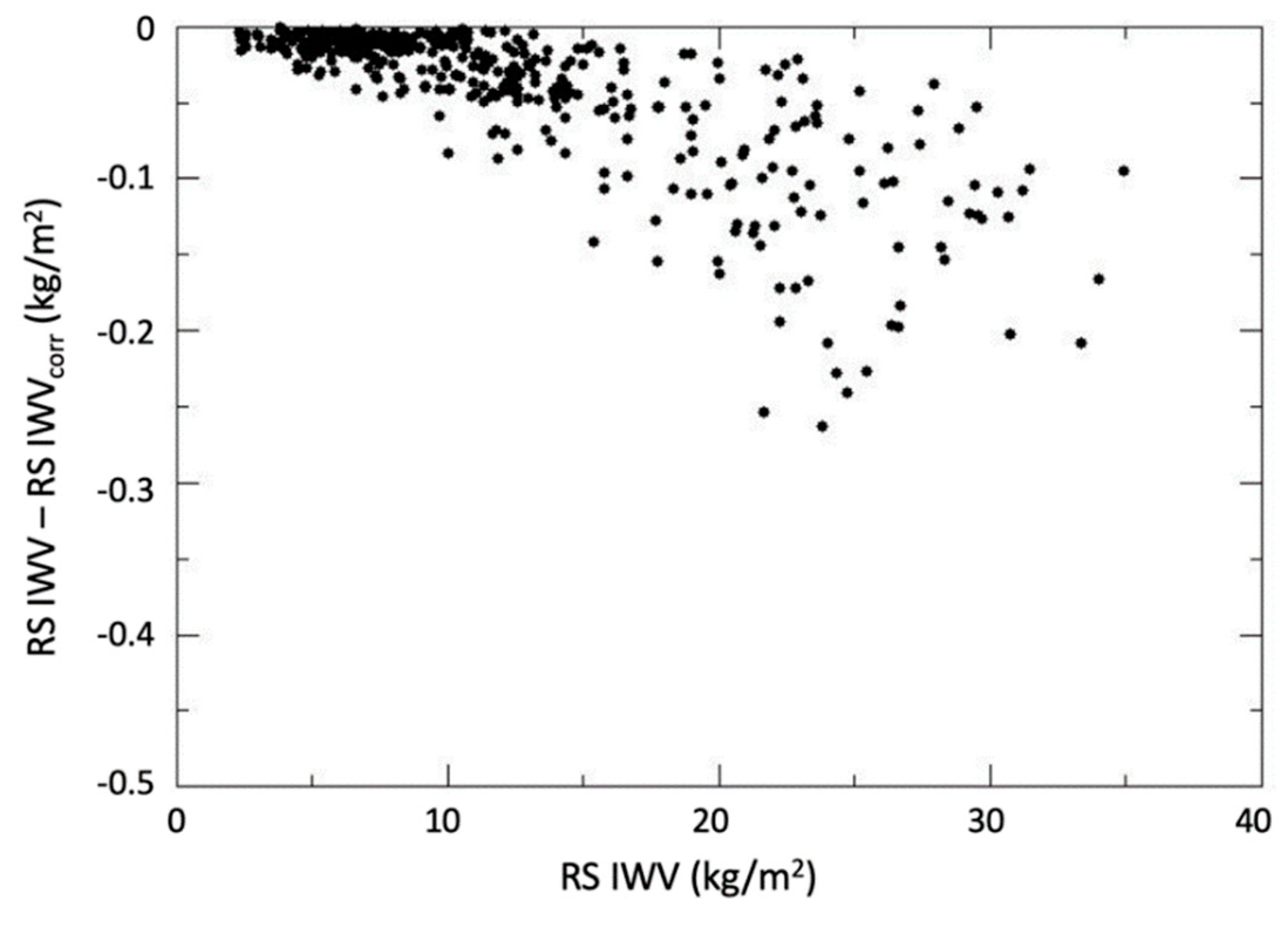
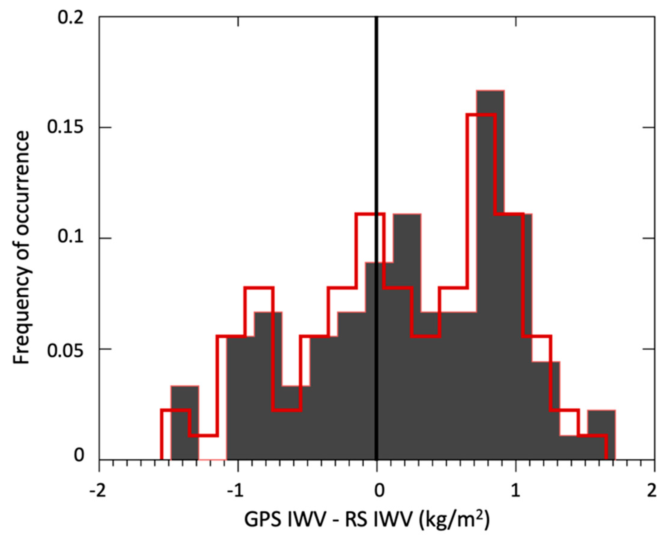
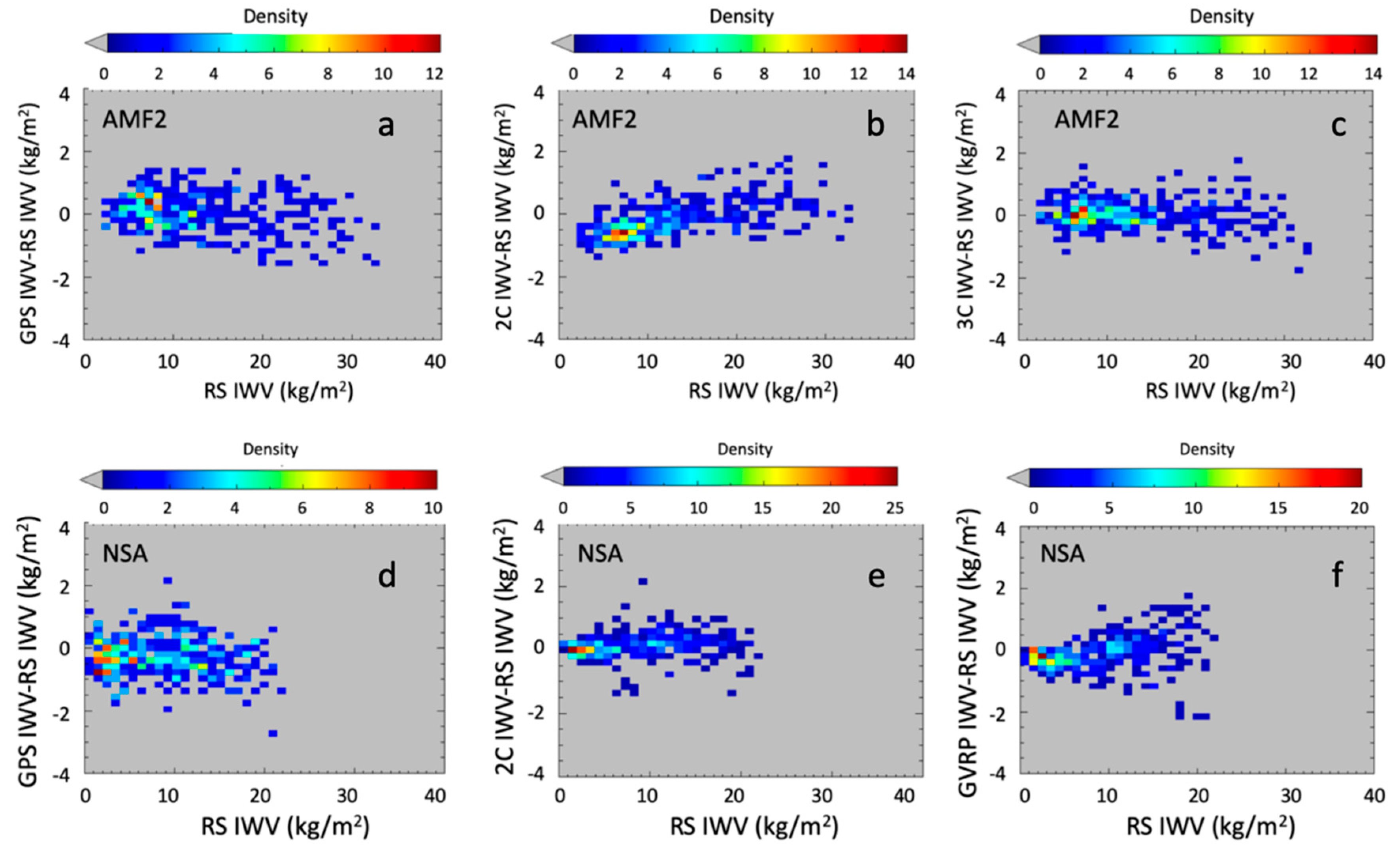
3.3. Comparison to Radiosondes

Radiosondes are launched regularly at both sites, twice per day at the NSA and four times per day at the AMF2 site. As mentioned in Section 2.1, the radiosondes are affected by a dry bias. Although the effect is more pronounced at lower latitudes, there are some small residual effects at higher latitudes [50]. The RS data were therefore corrected using the correction proposed by Wang et al. [29]. The differences between the original and corrected IWV were more pronounced at the AMF2 site and are shown in Figure 7 as a function of IWV. About 50% of the corrections were smaller than 0.02 kg/m². The magnitude of the differences at this site depended on the IWV and was comparable to what could be expected at midlatitude sites [50]. Although the correction may be relevant for individual launches, it had an overall small effect on the statistical distribution of the IWV. This was because cases with an IWV >15 g/m² and with solar elevation sufficient to induce an appreciable effect were few compared to the total number of cases. This is visible in Figure 8, where the IWV distributions before (solid gray) and after (red) the correction are shown for May–September 2014 at the AMF2, a time when the bias was largest. At the NSA, because the distribution was even more skewed toward low IWV values and because the sun elevation was lower, the effect of the correction was even smaller. Nonetheless, the radiosonde data in our comparisons were corrected for the dry bias effect.

An average of 30 min was performed on the radiometers and GPS data, starting from the radiosonde launch. Concurrent measurements at the NSA and AMF2 amounted to 414 and 397, respectively, with the relatively small number of radiosondes launched limiting the available number of points. The statistical parameters of the comparison between the radiosondes and the other sensors are shown in

Table 4. IWV statistical parameters of the radiosonde comparison (units are kg/m²). N is the number of points used at each site.

		AMF2 (N = 397)			NSA (N = 414)
	3C versus RS	GPS versus RS	2C versus RS	GVRP versus RS	GPS versus RS	2C versus RS
Bias	0.127	0.167	−0.134	−0.050	−0.178	0.210
SD	0.441	0.616	0.565	0.518	0.603	0.357
Slope	0.991	0.972	1.045	1.027	0.999	1.012
Offset	−0.471	1.244	0.649	0.026	−0.288	−0.341
R2	0.995	0.994	0.999	0.993	0.994	0.996

.

In Figure 9, the data are displayed in a manner similar to Figure 5. Overall, the density plots agree well with those of Figure 5. The AMF2 2C displayed a positive trend with RS IWV, confirming the temperature dependence previously discussed. The NSA GVRP displayed an effect of saturation when IWV >10 kg/m². The AMF2 3C had the best overall agreement with RS, with a bias of about 0.13 kg/m² and an SD of about 0.44 kg/m², showing almost no trend with respect to IWV. This confirmed the calibration quality of the instrument and the relevance of the 89.0-GHz channel at a high latitude. The bias comparison between the GPS and RS at AMF2 (Figure 9a) also showed a small negative trend with IWV, which was consistent with the small trend in the GPS comparison to the 3C (Figure 5c). This trend in the bias with respect to IWV was not noticeable at the NSA.

The GPS displayed the highest random variability. This latter feature is further shown in Figure 6 only for bins with more than 10 samples. At the AMF2 (black circles and squares in Figure 6d), the standard deviation between the RS and the GPS increased with increasing IWV more markedly than for the other instruments. At the NSA, the standard deviation of the differences did not depend on the IWV.

Although less statistically significant because of the smaller sample size, the RS comparison was very consistent with the radiometers and the GPS comparison at both sites. The effect of the larger GPS field of view could be seen at both sites as an increased SD between the GPS and the other sensors throughout the entire IWV range. At the AMF2 site, the larger GPS FOV as well as the distance between the GPS and the other instruments affected the comparison. In particular, the SD between the radiosondes and the radiometers (black circles and squares in Figure 6d) was between the SDs of the two co-located radiometers (black stars in Figure 6a) and the SDs of the GPS and the radiometers (black circles and squares in Figure 6a).

4. Discussion

Two datasets of concurrent 30-min IWV values from independent instruments (three ground-based radiometers with channels from 23 to 183 GHz, two GPS ground receivers, and Vaisala RS92 radiosondes) at two high-latitude sites (AMF2 in Finland and NSA in Alaska) were examined. The observations were collected in 2014 by several co-located and near-located instruments, and IWV values were inferred from each independent instrument in nonprecipitating atmospheric conditions. Vaisala RS92 radiosonde profiles were corrected for dry bias. The entire dataset composed by all data at both sites showed a high degree of consistency with an SD, bias, and R² of about 0.76 kg/m², 0.19 kg/m², and 0.995, respectively, in addition to a slope of 1.009. These general results can attest to the overall good and consistent quality of the data and are representative of high-latitude observations. At the single sites, a regression analysis evidenced the general agreement between the IWV measurements, with low biases ranging from −0.27 to 0.41 kg/m² and an SD ranging from about 0.44 to 0.68 kg/m², with a worst case of about 1 kg/m² for the AMF2 GPS versus the 2C. With respect to the RS, the SD values ranged from about 0.36 to 0.62 kg/m², with a variability of about 40%, and biases ranged from about −0.18 to 0.21 kg/m².

A deeper analysis of differences and the SD revealed some interesting features of the measurements. The GPS and the 3C at the AMF2 had the best agreement. The 2C at the AMF2, on the other hand, displayed a dependence on water vapor that was attributable to a slight residual temperature effect of the calibration. The enhanced sensitivity of 3C to small IWV amounts provided the overall best agreement with the GPS data and the RS, while the accuracy of the GVRP was limited to very dry conditions.

Most interestingly, the two sites showed different behavior in terms of the random variability and the systematic error, with the AMF2 site displaying an increase in the random variability and a small trend in the average differences between the GPS and other instruments. The trend in the average difference between the GPS and the 3C had a minimum value of −0.3 kg/m² in February and a maximum value of 0.28 kg/m² in August. The source of the trend was difficult to interpret due to its small magnitude and was likely due to the 20-km distance between the GPS and the AMF2 site. This was consistent with a pressure difference of around 1 mb between the two sites; however, it could also have been attributable to water vapor inhomogeneity.

The increase in the random variability could be attributed to atmospheric variability as well as to the distance between the GPS and the other instruments. The variability of the GPS differences at the AMF2 had a seasonal dependence displaying higher values in summer and lower values in winter. A similar behavior at midlatitudes was observed during times of higher water vapor in Haase et al. [49], which was attributed to the higher spatial variability of water vapor in summer. The analysis in this study seems to support that interpretation. The increased variability of the AMF2 differences seemed to be associated with conditions of increased water vapor and inhomogeneous cloudiness. Such dependence was not observed at the NSA site, where the instruments were strictly co-located and, although cloudiness is pronounced in summer, conditions in the GPS field of view were probably more homogeneous than in Finland.

The comparison between radiosondes, GPS, and radiometers, although less statistically significant because of the reduced dataset, was consistent with the 30-min dataset, with a positive trend. The standard deviation of the differences increased with increasing water vapor at the AMF2 and displayed no trend at the NSA. At both sites, however, the magnitude of the SD between the RS and radiometers was smaller than the SD between the GPS and radiometers. It was also noticeable that the larger difference between the two sites was in the comparison between the MWR and GPS. At AMF2, the SD assumed values slightly greater than at the NSA. This was probably due to the compounded effect of the 20-km distance between the GPS and the radiometers, which added to the difference in the FOV. The mean variability between the GPS and RS, on the other hand, was similar at both sites despite the 20-km distance between the GPS and the radiosonde launch site at the AMF2. The results suggest that the variability of the GPS measurements was dependent on location and regional climatology, and the effects of inhomogeneity in a GPS FOV may be the dominant component of the random variability of measurements even at high-latitude sites.

5. Conclusions

Understanding differences in water vapor measurements from different instruments benefits from the presence of multiple, independently calibrated sensors. However, differences in the sensor characteristics alone are not enough to interpret the comparisons. Measurements conducted at different sites with similar instrumentation help to understand features that may be external to the instrument characteristics. In particular, for instruments with large FOVs, such as the GPS, regional climatology plays an important role in the ability of the instrument to represent features at smaller spatial scales. The simultaneous use of co-located and near-located instrumentation can provide useful information when trying to understand the relative contribution of the instrument and of regional climatology to the variability of the measurements.

References

1. Allan, P.R. The Role of Water Vapour in Earth’s Energy Flows. Surv. Geophys. 2012, 33, 557–564. [Google Scholar] [CrossRef]
2. Basili, P.; Ciotti, P.; Fionda, E. Accuracy of physical, statistical and neural network based algorithms for the retrieval of atmospheric water by ground-based microwave radiometry. In Proceedings of the IGARSS’98, Seattle, WA, USA, 6–10 July 1998; pp. 418–420. [Google Scholar]
3. Mattioli, V.; Westwater, E.R.; Gutman, S.I.; Morris, V.R. Forward model studies of water vapor using scanning microwave radiometers, Global Positioning System, and radiosondes during the cloudiness intercomparison experiment. IEEE Trans. Geosci. Remote Sens. 2005, 43, 1012–1021. [Google Scholar] [CrossRef]
4. Elgered, G. Tropospheric radio-path delay from ground-based microwave radiometry. In Atmospheric Remote Sensing by Microwave Radiometry; Janssen, M.A., Ed.; John Wiley & Sons, Inc.: New York, NY, USA, 1993; Chapter 4; pp. 215–258. [Google Scholar]
5. Teke, K.; Nilsson, T.; Boehm, J.; Hobiger, T.; Steigenberger, P.; Garcia-Espada, S.; Haas, R.; Willis, P. Troposphere delays from space geodetic techniques, water vapour radiometers, and numerical weather models over a series of continuous VLBI campaigns. J. Geod. 2013, 87, 981–1001. [Google Scholar] [CrossRef]
6. Van Malderen, R.; Brenot, H.; Pottiaux, E.; Beirle, S.; Hermans, C.; De Mazière, M.; Wagner, T.; De Backer, H.; Bruyninx, C. A multi-site intercomparison of integrated water vapour observations for climate change analysis. Atmos. Meas. Tech. 2014, 7, 2487–2512. [Google Scholar] [CrossRef] [Green Version]
7. Choy, S.; Wang, C.-S.; Yeh, T.-K.; Dawson, J.; Jia, M.; Kuleshov, Y. Precipitable water vapor estimates in the Australian region from ground-based GPS observations. Adv. Meteorol. 2015, 2015. [Google Scholar] [CrossRef]
8. Memmo, A.; Fionda, E.; Paolucci, T.; Cimini, D.; Ferretti, R.; Bonafoni, S.; Ciotti, P. Comparison of MM5 integrated water vapor with microwave radiometer, GPS, and radiosonde measurements. IEEE Trans. Geosci. Remote Sens. 2005, 43, 1050–1058. [Google Scholar] [CrossRef]
9. Luini, L.; Riva, C. Improving the Accuracy in Predicting Water-Vapor Attenuation at Millimeter-Wave for Earth-Space Applications. IEEE Trans. Antennas Propag. 2016, 64, 2487–2493. [Google Scholar] [CrossRef]
10. ITU-R P.676-10. In Attenuation by Atmospheric Gases; International Telecommunications Union: Geneva, Switzerland, 2013; p. 24. Available online: https://www.itu.int/rec/R-REC-P.676-10-201309-S/en (accessed on 12 September 2019).
11. Witze, A. 5G data networks threaten forecasts Wireless technology could interfere with Earth observations. Nature 2019, 569, 17–18. [Google Scholar] [CrossRef]
12. Bedka, S.; Knuteson, R.; Revercomb, H.; Tobin, D.; Turner, D. An assessment of the absolute accuracy of the Atmospheric Infrared Sounder v5 precipitable water vapor product at tropical, midlatitude, and arctic ground-truth sites: September 2002 through August 2008. J. Geophys. Res. Atmos. 2010, 115. [Google Scholar] [CrossRef]
13. Alraddawi, D.; Sarkissian, A.; Keckhut, P.; Bock, O.; Noёl, S.; Bekki, S.; Irbah, A.; Meftah, M.; Claud, C. Comparison of total water vapour content in the Arctic derived from GNSS, AIRS, MODIS and SCIAMACHY. Atmos. Meas. Tech. 2018, 11, 2949–2965. [Google Scholar] [CrossRef] [Green Version]
14. Thomas, I.D.; King, M.A.; Clarke, P.J.; Penna, N.T. Precipitable water vapor estimates from homogeneously reprocessed GPS data: An intertechnique comparison in Antarctica. J. Geophys. Res. Atmos. 2011, 116, 1–18. [Google Scholar] [CrossRef]
15. Pałm, M.; Melsheimer, C.; Noël, S.; Heise, S.; Notholt, J.; Burrows, J.; Schrems, O. Integrated water vapor above Ny Ålesund, Spitsbergen: A multi-sensor intercomparison. Atmos. Chem. Phys. 2010, 10, 1215–1226. [Google Scholar] [CrossRef]
16. Berezin, I.A.; Timofeyer, Y.M.; Virolainen, Y.A.; Volkova, K.A. Comparison of ground-based microwave measurements of precipitable water vapour with radio sounding data. Atmos. Ocean. Opt. 2016, 29, 274–281. [Google Scholar] [CrossRef]
17. Buehler, S.A.; Östman, S.; Melsheimer, C.; Holl, G.; Eliasson, S.; John, V.O.; Blumenstock, T.; Hase, F.; Elgered, G.; Raffalski, U.; et al. A multi-instrument comparison of integrated water vapour measurements at a high latitude site. Atmos. Chem. Phys. 2012, 12, 10925–10943. [Google Scholar] [CrossRef] [Green Version]
18. Ning, T.; Haas, R.; Elgered, G.; Willen, U. Multi-technique comparison of 10 years of wet delay estimates on the west coast of Sweden. J. Geod. 2012, 86, 565–575. [Google Scholar] [CrossRef]
19. Miloshevich, L.M.; Vomel, H.; Whitman, D.N.; Leblanc, T. Accuracy assessment and correction of Vaisala RS92radiosonde water vapour measurements. J. Geophys Res. 2009, 114. [Google Scholar] [CrossRef]
20. Atmospheric Radiation Measurement Program, Biogenic Aerosols-Effects on Clouds and Climate (BAECC) Campaign. Available online: https://www.arm.gov/research/campaigns/amf2014baecc (accessed on 2 August 2019).
21. Cadeddu, M.P.; Liljegren, J.C.; Turner, D.D. The Atmospheric Radiation Measurement (ARM) program network of microwave radiometers: Instrumentation, data, and retrievals. Atmos. Meas. Tech. 2013, 6. [Google Scholar] [CrossRef]
22. Racette, P.E.; Westwater, E.R.; Han, Y.; Gasiewski, A.J.; Klein, M.; Cimini, D.; Jones, D.C.; Manning, E.J.; Kim, W.; Wang, J.R.; et al. Measurement of Low Amounts of Precipitable Water Vapor Using Ground-Based Millimeter wave Radiometry. J. Atmos. Ocean. Technol. 2005, 22, 317–337. [Google Scholar] [CrossRef]
23. Wu, S.-C. Optimum frequencies of a passive microwave radiometer for tropospheric path-length correction. IEEE Trans. Antennas Propag. 1979, 27, 233–239. [Google Scholar]
24. Westwater, E.R.; Guiraud, F.O. Ground-based microwave radiometric retrieval of precipitable water vapor in the presence of clouds with high liquid content. Radio Sci. 1980, 15, 947–957. [Google Scholar] [CrossRef]
25. Ulaby, F.T.; Moore, R.K.; Fung, A.K. Microwave Remote Sensing, Active and Passive. In Microwave Remote Sensing Fundamentals and Radiometry; Addison-Wesley Publishing Company: Reading, MA, USA, 1981; Volume 1. [Google Scholar]
26. Mattioli, V.; Basili, P.; Bonafoni, S.; Ciotti, P.; Westwater, E.R. Analysis and improvements of cloud models for propagation studies. Radio Sci. 2009, 44, RS2005. [Google Scholar] [CrossRef]
27. Wang, J.; Zhang, L. Systematic errors in global radiosonde precipitable water data from comparisons with ground-based GPS measurement. J. Clim. 2008, 21, 2218–2238. [Google Scholar] [CrossRef]
28. Cady-Pereira, K.; Shephard, M.W.; Turner, D.D.; Mlawer, E.J.; Clough, S.A.; Wagner, T.J. Improved daytime column-integrated precipitable water vapor from Vaisala Radiosonde Humidity Sensors. J. Atmos. Appl. Technol. 2008, 25, 873–883. [Google Scholar] [CrossRef]
29. Wang, J.; Zhang, L.; Dai, A.; Immler, F.; Sommer, M.; Vomel, H. Radiation dry bias correction of Vaisala RS92 humidity data and its impacts on historical radiosonde data. J. Atmos. Ocean. Technol. 2013, 30, 197–214. [Google Scholar] [CrossRef]
30. Peppler, R.A.; Long, C.N.; Sisterson, D.L.; Turner, D.D.; Bahrmann, C.P.; Christensen, S.W.; Doty, K.J.; Eagan, R.C.; Halter, T.D.; Ivey, M.D.; et al. An overview of ARM Program Climate Research Facility data quality assurance. Open Atmos. Sci. J. 2008, 2, 192–216. [Google Scholar] [CrossRef]
31. Peppler, R.A.; Kehoe, K.E.; Monroe, J.W.; Theisen, A.K.; Moore, S.T. The ARM Data Quality Program. Meteorol. Monogr. 2016, 57, 12.1–12.14. [Google Scholar] [CrossRef]
32. Saastamoinen, J. Atmospheric correction for the troposphere and stratosphere in radio ranging satellites. In The Use of Artificial Satellites for Geodesy, 1st ed.; Henriksen, S.W., Mancini, A., Chovitz, B.H., Eds.; Geophysical Monograph Series; American Geophysical Union: Washington, DC, USA, 1972. [Google Scholar]
33. Davis, J.L.; Herrin, T.A.; Shapiro, I.I.; Rogers, A.E.E.; Elgered, G. Geodesy by radio interferometry: Effects of atmospheric modelling errors on estimates of baseline length. Radio Sci. 1985, 20, 1593–1607. [Google Scholar] [CrossRef]
34. Ning, T.; Wang, J.; Elgered, G.; Dick, G.; Wickert, J.; Bradke, M.; Sommer, M.; Querel, R.; Smale, D. The uncertainty of the atmospheric integrated water vapour estimated from GNSS observations. Atmos. Meas. Tech. 2016, 9, 79–92. [Google Scholar] [CrossRef] [Green Version]
35. Bevis, M.; Businger, S.; Herring, T.A.; Rocken, C.; Anthes, R.A.; Ware, R.H. GPS meteorology: Remote sensing of atmospheric water vapor using the global positioning system. J. Geophys. Res. 1992, 97, 15787–15801. [Google Scholar] [CrossRef]
36. Basili, P.; Bonafoni, S.; Ferrara, R.; Ciotti, P.; Fionda, E.; Ambrosini, R. Atmospheric water vapor retrieval by means of both a GPS network and a microwave radiometer during an experimental campaign in Cagliari, Italy, in 1999. IEEE Trans. Geosci. Remote Sens. 2001, 38, 2436–2443. [Google Scholar] [CrossRef]
37. Pierdicca, N.; Guerriero, L.; Giusto, R.; Broioni, M.; Egido, A. SAVERS: A Simulator of GNSS reflections from bare and vegetated soils. IEEE Trans. Geosci. Remote Sens. 2014, 52, 6542–6554. [Google Scholar] [CrossRef]
38. Zumberge, J.F.; Heflin, M.B.; Jefferson, D.C.; Watkins, M.M.; Webb, F.H. Precise point positioning for the efficient and robust analysis of GPS data from large networks. J. Geophys. Res. 1997, 102, 5005–5017. [Google Scholar] [CrossRef] [Green Version]
39. Webb, F.H.; Zumberge, J.F. An Introduction to GIPSY/OASIS II, Jet Propulsion Laboratory Document JPL D-11088; California Institute of Technology: Pasadena, CA, USA, 1997; Available on request. [Google Scholar]
40. Pacione, R.; Pace, B.; Bianco, G. Homogeneously reprocessed ZTD long-term time series over Europe. In Proceedings of the EGU GA 2014, Vienna, Austria, 27 April–2 May 2014; Available online: http://meetingorganizer.copernicus.org/EGU2014/EGU2014-2945.pdf (accessed on 12 september 2019).
41. Pacione, R.; Araszkiewicz, A.; Brockmann, E.; Douša, J. EPN-Repro2: A reference GNSS tropospheric data set over Europe. Atmos. Meas. Tech. 2017, 10, 1689–1705. [Google Scholar] [CrossRef] [Green Version]
42. Boehm, J.; Werl, B.; Schuh, H. Troposphere mapping functions for GPS and very long baseline interferometry from European Centre for Medium-Range Weather Forecasts operational analysis data. J. Geophys. Res. 2006, 111. [Google Scholar] [CrossRef]
43. Verlinde, J.; Zak, B.D.; Shupe, M.D.; Ivey, M.D.; Stamnes, K. The ARM North Slope of Alaska (NSA) Sites. Meteorol. Monogr. 2016, 57, 8.1–8.13. [Google Scholar] [CrossRef]
44. Cadeddu, M.P.; Turner, D.D.; Liljegren, J.C. A Neural Network for Real-Time Retrievals of PWV and LWP from Arctic Millimeter-Wave Ground-Based Observations. IEEE Trans. Geosci. Remote Sens. 2009, 47, 1887–1900. [Google Scholar] [CrossRef]
45. Ware, R.H.; Fulker, D.W.; Stein, S.A.; Anderson, D.N.; Avery, S.K.; Clark, R.D.; Droegemeier, K.; Kuettner, J.P.; Minster, J.B. Suominet: A real-time national GPS network for atmospheric research and education. Bull. Am. 2000, 81, 677–694. [Google Scholar] [CrossRef]
46. Dach, R.; Lutz, S.; Walser, P.; Fridez, P. Bernese GNSS Software Version 5.2. University of Bern: Bern, Switzerland, 2015. Available online: http://www.bernese.unibe.ch/docs/DOCU52.pdf (accessed on 12 September 2019).
47. King, R.; Herring, T.; Mccluscy, S. Documentation for the GAMIT GPS Analysis Software 10.4; Tech. Rep.; Massachusetts Institute of Technology: Cambridge, MA, USA, 2010. [Google Scholar]
48. Cole, A.E.; Court, A.; Kantor, A.J. Model Atmospheres. In Handbook of Geophysics and Space Environments; Valley, S.L., Ed.; Office of Aerospace Research, USAF: Hanscom AFB, MA, USA, 1965; Chapter 2. [Google Scholar]
49. Haase, J.; Ge Vedel, M.; Calais, E. Accuracy and variability of GPS tropospheric delay measurements of water vapor in the western Mediterranean. J. Appl. Meteorol. 2003, 42, 1547–1568. [Google Scholar] [CrossRef]
50. Dzambo, A.M.; Turner, D.D.; Mlawer, E.J. Evaluation of two Vaisala RS92 radiosonde solar radiative dry bias correction algorithms. Atmos. Meas. Tech. 2016, 9, 1613–1626. [Google Scholar] [CrossRef] [Green Version]
Figure 1. (a) From left to right, 2C and 3C radiometers at the AMF2 site (Hyytiälä, Finland). The enclosure near the three-channel radiometer (3C) contains the control computer, meteorological sensors, and infrared thermometer. (b) A view of the north slope of Alaska (NSA) facilities in Barrow, Alaska (USA): in the foreground the G-Band Vapor Radiometer Profiler (GVRP), in the background the 2C radiometer.
Remotesensing 11 02130 g001
Figure 2. Latitude and longitude of the NSA (a) and AMF2 (b) sites (black star), the GPS (black square), and the RS at an 8-km height. The shaded brown area represents the approximate FOV of the GPS for a cut-off angle of 3°. The star and square overlap at the NSA.
Remotesensing 11 02130 g002
Figure 3. (a) Scatterplot of the IWV from the GPS (x axis) and from all operated radiometers (y axis) at the NSA (blue) and AMF2 (orange). The dashed black line represents a 1:1 ratio. (b) The number of occurrences of absolute differences between the microwave radiometers (MWRs) and the GPS. The red solid line represents the normal distribution fit. The normal distribution had a mean of 0.191 kg/m2 [0.181, 0.200] with an SD of 0.756 kg/m2 [0.750, 0.763]. The intervals next to the parameter estimates are the 95% confidence intervals for the distribution parameters.
Remotesensing 11 02130 g003
Figure 4. (a): Monthly mean of differences; (b) monthly mean of the standard deviation of the differences.
Remotesensing 11 02130 g004
Figure 5. Density plots of differences between: (a) 3C and GPS at AMF2; (b) 2C and GPS at AMF2; (c) 3C and GPS at AMF2; (d) GVRP and GPS at NSA; (e) 2C and GPS at NSA; (f) GVRP and 2C at NSA. All difference binned by IWV bins of 5 kg/m2.
Remotesensing 11 02130 g005
Figure 6. Left three panels: GPS and radiometers comparison. (a) Standard deviation of differences as a function of IWV; (b) percent of cloudy cases; (c) number of cases in each bin. Right panels: RS, GPS, and radiometers comparison. (d) Standard deviation of differences as a function of IWV; (e) number of cases in each bin. In all panels, IWV bins are 5 kg/m2, brown symbols refer to the NSA, and black symbols refer to the AMF2.
Remotesensing 11 02130 g006
Figure 7. Differences between original and corrected IWV (kg/m2) at the AMF2 (all data).
Remotesensing 11 02130 g007
Figure 8. Distribution of daytime (11:00–17:00 UTC) GPS–RS mean differences before (gray) and after (red) the dry bias correction at the AMF2 (data are for May–September 2014).
Remotesensing 11 02130 g008
Figure 9. Density plots of differences between: (a) GPS and RS at AMF2; (b) 2C and RS at AMF2; (c) 3C and RS at AMF2; (d) GPS and RS at NSA; (e) 2C and RS at NSA; (f) GVRP and RS at NSA. All difference binned by IWV bins of 5 kg/m2.
Remotesensing 11 02130 g009