Article

Irrigation Optimization Under a Limited Water Supply by the Integration of Modern Approaches into Traditional Water Management on the Cotton Fields

1
Spectroscopy and Remote Sensing Laboratory, Center for Spatial Analysis Research (UHCSISR), Department of Geography and Environmental Studies, University of Haifa, Aba Hushi, 199-3498838 Haifa, Israel
2
National Research Council of Italy (CNR), Institute for Mediterranean Agricultural and Forestry Systems (ISAFOM), Via Patacca, 85-80056 Ercolano (NA), Italy
*
Author to whom correspondence should be addressed.
Remote Sens. 2019, 11(18), 2127; https://doi.org/10.3390/rs11182127
Submission received: 31 July 2019 / Revised: 2 September 2019 / Accepted: 5 September 2019 / Published: 12 September 2019

Abstract

:
The ability to effectively develop agriculture with limited water resources is an important strategic objective to face future climate change and to achieve the Sustainable Development Goal 2 (SDG2) of the United Nations. Since new conditions increasingly point to a limited water supply, the aim of modern irrigation management is to be sure to maximize the crop yield and minimize water use. This study aims to explore the advantages of the traditional agronomic approach, agro-hydrological model and field feedback obtained by spectroscopy, to optimize irrigation water management in the example of a cotton field. The study was conducted for two summer growing seasons in 2015 and 2016 in Kibbutz Hazorea, near Haifa, Israel. The irrigation schedule was developed by farmers using weather forecasts and corrected by the results of field inspections. The Soil Water Atmosphere Plant (SWAP) model was applied to optimize seasonal water distribution based on different criteria (critical soil pressure head and allowable daily stress). A new optimization algorithm for irrigation schedules by weather forecasts and vegetation indices was developed and presented in this paper. A few indices related to physical parameters and plant health (Normalized Difference Vegetation Index, Red Edge Normalized Difference Vegetation Index, Modified Chlorophyll Absorption Ratio Index 2, and Photochemical Reflectance Index) were considered. Red Edge Normalized Difference Vegetation Index proves itself as a suitable parameter for monitoring crop state due to its clear-cut response to irrigation treatments and was introduced in the developed algorithm. The performance of the considered irrigation scheduling approaches was assessed by a simulation model application for cotton fields in 2016. The results show, that the irrigation schedule developed by farmers did not compensate for the absence of precipitation in spring, which led to long-term lack of water during crop development. The optimization developed by SWAP allows determining the minimal amount of water which ensures appropriate yield. However, this approach could not take into account the non-linear effect of the lack of water at specific phenological stages on the yield. The new algorithm uses the minimal sufficient seasonal amount of water obtained from SWAP optimization. The approach designed allows one to prevent critical stress in cotton and distribute water in conformity with agronomic practice.

Graphical Abstract

1. Introduction

Agriculture and agricultural landscapes are increasingly under pressure to meet the demands of a constantly increasing human population and globally changing food patterns. Moreover, to this is added, the expected reduction of global agricultural land availability [1] and the necessity to achieve food security by means of double the agricultural productivity by 2030 under changing climate conditions (Sustainable Development Goal 2—SDG2, of United Nations). As a result, there are rising concerns that climate change and food security will harm agriculture in many regions of the world by changing the land use, soil degradation, and intensive uses of pesticides and fertilizers [2].
Crop production depends on solar radiation and is greatly affected by temperature and rainfall [3] to the point that water shortage represents the most important environmental factor limiting crop growth, development and yield [4,5]. Then, well-timed availability of water is vital to ensure crop yields and the efficiency of several agricultural inputs (e.g., seeds, fertilizers and pesticides).
Moreover, considering that in the last century water use has been growing globally at more than twice the rate of population increases and that the first sector affected by water shortage is agriculture, resulting in a decreased capacity to maintain per capita food production [6], an optimization of water resource use is one of the most important aims to face the future climate change and food security. Therefore, the need arises for optimal irrigation scheduling techniques that coordinate the timing and amount of irrigation to optimally manage the water use in agriculture systems.
The advantages of a proper irrigation scheduling are not only in the maximizing of crop yield but also in time and energy saving, that allow all to preserve environment health (e.g., nitrogen and pesticides leaching to groundwater). Many studies have concluded that optimal irrigation decisions can provide substantial economic value over conventional irrigation decisions [7,8]. The main challenge in the identification of a correct irrigation scheduling is attributed to the uncertainty of factors involved in the soil–plant and atmosphere system processes during the growing season. Most notably, the climatic factors, such as evapotranspiration and rainfall and soil physical characteristics. Currently, advancements in short-term and mid-term weather forecasting have reduced the uncertainty level associated with future climatic data, and accordingly, agricultural management has started to use meteorological stations, to improve the irrigation scheduling. For the calculation of water consumption based on meteorological data and to make an accurate irrigation plan, the method of Allen [9] based on the potential evapotranspiration (ET0) in common with a specific crop parameter named crop coefficient (Kc) data is used. However, this method does not allow one to plan irrigation in the case of water constraints and is orientated to maximize absolute yield without accounting for the productivity of amount of water per yield [10]. To compensate these shortcomings and reduce water consumption, irrigation management has to be supported by field feedback to achieve optimal crop development [11].
The field feedback about optimal crop development can be estimated by means parameters as the timely occurrence of certain phenological stages and crop growth rate [12], leaf water potential [13], and appropriate soil water content [14]. The accuracy of the evaluation of the above parameters is directly related to the cost of their measurements. For example, methods based on visual inspection and measuring basic physical parameters (e.g., plant height, leaf area index, leaf angle distribution) are most common because of their simplicity and affordability, although the accuracy of the assessment is low and does not allow one to identify stress in the early stages. Advanced and progressive methods, such as leaf or steam water potential and stomatal conductance, relative leaf water content and light use efficiency might overperform those basic crop parameters and identify stress at an early stage.
One more modern monitoring technology able to detect stress early stress is spectroscopy. Examining plants by their spectrum is an attractive approach for agriculture needs because it is a non-destructive method for estimating a wide range of crop properties (e.g., vegetation cover, plant biomass, green leaf area index (LAI) and other biophysical characteristics; [15]), detecting stresses and diseases [16,17,18] by vegetation indices (VIs) and spectral models, with high temporal, spatial and spectral resolution (high spectral resolution—1 nm; wide wavelengths range across visible, near-infrared and short-wave infrared ranges—VIS, NIR, and SWIR). The spectrum provides the information about different physical parameters, pigment composition and plant metabolism at once. However, such measures are more complex and more qualified personnel are required than for measures of the single parameter; e.g., stomatic conductance and stem/leaf water potential. Despite the ability to correct watering according to the plant water state, none of the selected approaches for crop status assessment are able to solve the problem of planning irrigation for a long period.
Simulation models of the soil–plant and atmospheric system can allow one to face and solve this problem, supporting long-term irrigation planning [10]. In the past few decades, the dynamics of crop growth models have made substantial progress, and many crop models are available. Many models exist for predicting how crops respond to climate, nutrients, water, light and other conditions. New modeling approaches have tried to improve the classical models by replacing descriptions of individual processes and their interactions based on newly understood physiological mechanisms [19,20]. Crop growth modeling determines dry matter accumulation (or potential production) with three principal approaches: a carbon-driven, solar-driven or water-driven growth-engine. The last is considered as more suitable for irrigation and water-use assessments.
Nowadays there are several simulation models and decision support systems (DSS) for agricultural needs [21]. They differ in their mathematical formulations, structures and complexities and consist of a unique combination of empirical and mechanistic concepts [22,23]. Among the well-known models for irrigation planning, there is SWAP [24], WOFOST [25] and AquaCrop [26]. Each model has its own pros and cons in the application. For example, the strength points of AquaCrop are the crop growth engine and the needing of little soil information for a simulation run; using data easily present in any soil database (wilting point, field capacity, etc.). On the other hand, how the model solves the soil water balance (by means of a cascade model) could be considered a weak point in some real applications. WOFOST has a wide database of crops for detailed simulation and three approaches to solve the soil water balance. The strength of WOFOST is the application of different sets of crop growth parameters as a function of development stage that provides accurate simulation of crop biomass growth [27]. Despite the highly accurate crop simulation, the simulated WOFOST soil water balance is less easily performed than in other simulation models [28]. SWAP model is strong in the solving of the soil water balance by means of Richards equations, while its weak points could be considered how it simulates crop development (simple crop model or detailed crop model borrowed from the WOFOST) and its need of detailed soil information for a simulation run (e.g., soil description, hydraulic properties of soil horizons, etc.). All above models allow one to make an irrigation schedule according to the different crop stress (e.g., ratio between actual and potential plant transpiration, and pressure head at specific soil depth) and then provide the timing and the amount of water for irrigation.
Despite a large variety of simulation models available, their practical use is not diffuse because their application needs specific field parameters not available for farmers [29] and high user know-how; moreover, their use is discouraged because in many cases the simulated irrigation results are very similar to what farmers do normally in practice [30,31]. Not less important, it is the fact that all risks of yield cutback in case of incorrect irrigation scheduling lie only on farmers, thus in practice, preference is given to experience and traditional well-known approaches, rather than simulation models that do not respond to the actual field state and do not take into account the specificity of crop phenological development. Scientific studies have confirmed that reducing irrigation at various stages of development has a different effect on yield and this parameter is unique for different crop species [32]. For example, cotton yield is most sensitive for lack of water at emergence and fruit formation stages [33]. At the same time, it is necessary to consider the duration of water stress, as a prolonged water deficit significantly reduces the yield, regardless of the phenological stage [34,35]. Another feature of cotton irrigation management is yield increase due to water reduction at specific stages: It is explained by a negative correlation between cotton height and yield [36]. Thus, artificially created water stress is a common practice in growing cotton in order to contain excessive plant growth.
The purpose of this study is to evaluate the advantages of traditional irrigation management in combination with modern approaches, such as spectral indices and simulation models’ applications to support the optimization of irrigation scheduling. The aim of the study will be achieved through the examination of current methods for irrigation planning and developing an irrigation algorithm able to include the advantages of each considered approach. The performance of irrigation schedule developed by the considered methods is assessed by the SWAP simulation model.

2. Materials and Methods

2.1. Study Area

The study was conducted for two summer growing seasons in 2015 and 2016 on cotton fields. The monitored fields were situated in Kibbutz Hazorea, near Haifa, Israel (32°38′42.0″N 35°07′17.6″E). The climate classification of the study area is Mediterranean, with warm winters (average daily temperature ranging from +9 °C to 30 °C; and heavy rain, 92–136 mm per month) and dry hot summers (average temperature ranging from 21 °C to 31 °C with no rain). Moreover, in the observed region, monthly mean daily evaporation in summer varies from 10 mm to 11 mm by Class A evaporation pan method (ET0). Particularly, in growth season 2015, the mean daily temperature was 22.7 ± 6.1 °C. Slightly higher values were observed in 2016: the mean daily temperature was 23.3 ± 5.8 °C. During the cotton growth in 2015 the total amount of precipitation was 93 mm; 63% of it fell on April 10 and 11. In 2016, during growth period the total amount was 40 mm and 33% fell on April 12.
According to the USDA Soil Taxonomy, the soil in the Kibbutz Hazorea was identified as Vertisol [37]. This soil has heavy texture and high moisture-holding capacity (60%). Consistent with data from Israel Ministry of Agriculture, the soil texture on the observed cotton fields is clay, 54%, and Montmorillonite clay, 64%, out of which, silt is 31%, and sand 15%. Vertisol is known to be suitable for agriculture, but it requires accurate irrigation management [38]. Excessive drying of Vertisol can negatively effect on plant roots, due to the swelling and shrinkage processes; therefore, irrigation practice for this soil is to frequently irrigate.

2.2. Agronomic Managment

The cotton spice and basic principles management were the same in both monitored years. Cotton (Gossypium hirsutum L. ‘HA-195′, hybrid by Hazera seeds Ltd.) was planted with the distance between rows of 90 cm and rows and had a north/south direction. The planting of seeds was with a density of 7 kg ha−1 and the cover area was nearly 13 ha. In 2015, cotton was planted on the March 18 and in 2016 it was planted on the March 23. The harvesting started on October 5 in both years. The irrigation was carried out by surface drip with seasonal water limitation of 5000 m3 ha−1. The weekly amount of water was divided into three irrigation events (one every two days). The first two portions of watering were 40% for each one and last was 20%. This principle was found empirically by farmers as optimal to ensure the constant moistening of Vertisol on the one hand, and to minimize the loss of water by evaporation due to frequent watering on the other hand. The basic irrigation amount of water for season scheduling was calculated as water consumption by crop evapotranspiration (Equation (1)):
ETc = Kc·ET0
where ETc is crop evapotranspiration, ET0 is reference evapotranspiration by Class A evaporation pan method, and Kc is the crop coefficient provided by cotton growth guide [39].
The calculated daily water consumption was summarized to weekly amount of water. The estimated weekly amount of water for irrigation was corrected by field feedback. Farmers from Hazorea used daily crop growth rate and actual crop phenological state as field feedback parameters. The actual height was compared with reference from the crop guide [39]. In case of significant deviations in the growth rate, the weekly amount of water was changed: declined when the rate was too high and increased when the rate was to law. The actual phenological stage was used for estimation of the optimal time of the first irrigation and further correction of the crop coefficient.

2.3. Field Data Collection

In addition to the agronomic field inspections, the plants were examined by portable field spectrometer. The cotton’s spectral measures were obtained by the spectrometer (USB4000, Ocean Optics Inc, Dunedin, FL, USA) acquiring data across the VIS and NIR range from 350 to 1100 nm with a resolution of 0.5 nm and accuracy of 1 nm. The spectrometer’s calibration was carried out with Spectralon plate (Labsphere Inc., North Sutton, NH, USA) according to the protocol [40]. The spectral data was collected by a bare fiber optic with 25° field-of-view positions at a nadir view angle. The measurements were on the leaf-scale: the distance between the fiber and crops was approximately 5–10 cm; the chosen leaves were orientated perpendicularly relative to the sun. The campaigns were carried out between 11:00 and 13:00 o’clock when cloud cover was less than 10%. The series of measurements were conducted several times during each irrigation period (2015 and 2016). The observations were carried out by grid mission on the area 20 × 20 m.
The agronomist provided the information about crop development and irrigation scheduling according to the description in the cotton growth guide [39]. The estimations of cotton health and detection stress were conducted during field visual inspections according to plant-based irrigation scheduling methods [41]. The agronomic inspection includes identification an actual phenological stage based on the plant structure and health assessment by leaf parameters (color, dryness, texture and shape). The results of observations were compared with reference values for specific days of growth from the crop guide [39] to evaluate plant state. In addition to agronomic inspections, several representative plants were selected in a control plot (20 × 20 m), and their heights were measured for the estimation of the growth rate.

2.4. Spectral Data Analysis

The average spectrum was calculated from spectral measurements obtained on the control plot from one date. The resulting spectrum was used to calculate VIs. For monitoring crop state there were four indexes chosen for their responses to plant health and greenness (Table 1): Normalized Difference Vegetation Index (NDVI), Red Edge Normalized Difference Vegetation Index (RENDVI), Modified Chlorophyll Absorption Ratio Index 2 (MCARI2), and Photochemical Reflectance Index (PRI). In this study, there were VIs used for their responses to physical plant characteristics (green biomass and LAI), pigmentation (chlorophyll) and plant activity (photosynthesis). Except for the direct application for the estimation of physical parameters these indices also applied in spectral models for the estimation of crop water state, and detecting water and nutrient stress [42,43,44,45].

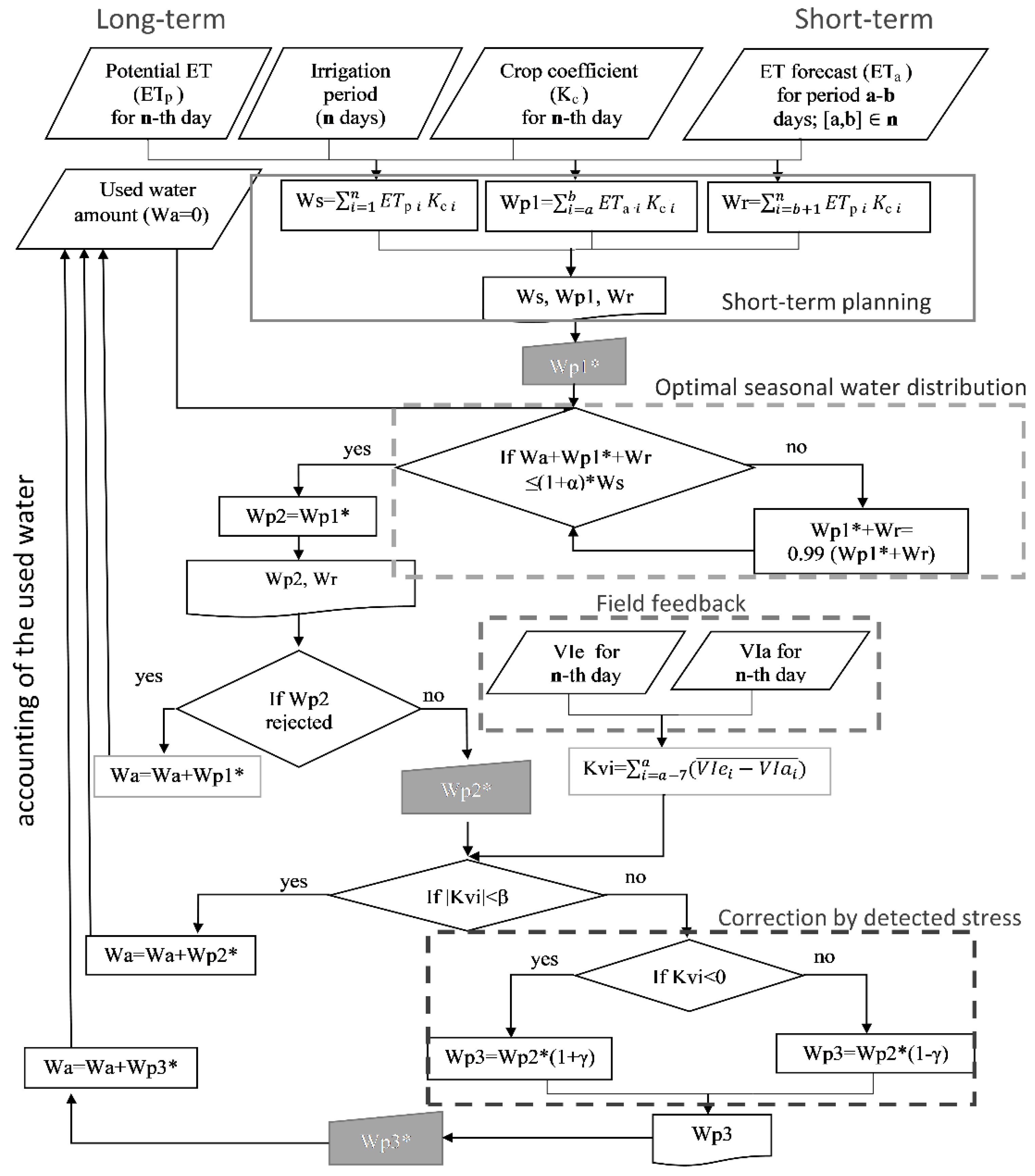
2.5. Optimization by Weather Forecast and Field Spectroscopy

A new optimization algorithm was developed to improve the existing method used on the monitored fields. In practice, amount of water was calculated based on the weekly weather forecast and then corrected by the outcome results of field agronomic inspection (correspondence of the growth rate and leaves’ parameters to crop growth guide description [41]). Practiced weekly planning without considering long-term perspectives led to water over-consumption in the first half of the season and shortage in the remaining period. The developed algorithm (Figure 1) was proposed to improve field state estimation by spectroscopy and combine a short-term planning by weather forecasts with ensuring a proportional water distribution throughout the season. The optimization consists of three parts.
The first step is long- and short-term irrigation planning using the weather forecast. For the estimation of irrigation the amount of water used the traditional water consumption method: multiplying ET0 by Kc. The seasonal irrigation amount (Ws) is defined by potential ET (ETp) for irrigation period (n days) and Kc provided for a specific crop. Input weather data can be used historical averages, data from the previous year or long-term (seasonal) forecast. This multi-variation of meteorological inputs provides an estimate of water and economic costs when a long-term forecast is not available. A calculation of the seasonal amount of water is needed to assess potential water use and plan proportional water distribution during the season. The optimization starts, when a user introduces a short-term weather forecast—actual ET (ETa). The term (a–b days) is defined by the user according to the available forecast. The algorithm calculates recommended amount of water (Wp1) for the defined term by ETa and the water residues until the end of the season based on ETp (Wr). At the end of this stage, the algorithm requests confirmation of Wp1 from the user and gives the opportunity to introduce an alternative value. Approved amount of water for the defined term (Wp1*) is introduced to the further optimization.
The second step is the optimization seasonal water distribution. Since the seasonal amount of water (Ws) is considered to be a constant, introducing Wp1* can lead to water overrun and significant reduction the amount of water for the remaining period (Wr). To avoid this, the algorithm checks that estimated total amount of water does not exceed Ws more than threshold value (α). The total amount of water is calculated as a sum of Wp1, Wr and already used water (Wa). Initially, Wa is defined as zero, and updates when irrigation amounts for the planned period (a–b days) is accepted. In case of excess, the algorithm proportionally reduces the Wp1 and Wr to fit the Ws. When the reduced values satisfy the conditions, the updated recommended amount of water (Wp2) is presented to the user with recalculated Wr. Accepted Wp2 turns to Wp2* and is used for the next optimization stage. In case of disagreement, the user can introduce Wp2 by himself or start a new process with new inputs or Wp1. If Wp2 is rejected, the algorithm considers Wp1 as accepted and adds it to the used amount of water (Wa).
The third step is intended to introduce field feedback for development optimal irrigation. In this study, VIs were used as the crops’ water-need parameter. This part could be modified according to available data: crop growth rate, plant water potential, soil moisture, etc. The algorithm requires reference values of the control parameter (VIe) and a value obtained from the field during the week before the planned period of irrigation (VIa). The difference between VIe and VIa is calculated and normalized to define the deviation of actual value from the expected. In the case of significant deviation (more than threshold β) the planned irrigation amount of water (Wp3) increases or decreases by γ depending on the actual crop water state. The results of the estimated amount of water for the planned period passes user approval like at previous step.

2.6. Agro-Hydrological Simulation Model

For the propose of this study the agro-hydrological model SWAP version 4.0.1 [24] was chosen. SWAP is an integrated physically-based simulation model of water, solute and heat transport in the saturated–unsaturated zone in relation to crop growth. In this study, only the water flow module was used; it assumes 1-D vertical flow processes and calculates soil water flow through the Richards’ equation. Soil water retention is described by the unimodal θ (h) relationship proposed by Van Genuchten [49] and expressed in terms of effective saturation, Se. Mualem’s expression [50] is applied to calculate relative hydraulic conductivity, Kr. Assuming m = 1 − 1 n−1, Van Genuchten [49] obtained a closed-form analytical solution to predict Kr at a specified volumetric water content. The condition at the bottom boundary can be set in several ways (pressure head, water table height, fluxes, impermeable layer, unit gradient, etc.).
The upper boundary conditions of SWAP in agricultural crops are generally described by the potential evapotranspiration ET0, irrigation and daily precipitation. Therefore, the potential evapotranspiration is partitioned into potential soil evaporation, Ep, and potential transpiration, Tp, according to the LAI evolution, following the Ritchie approach [51].
SWAP simulates water uptake and actual transpiration according to the model proposed by Feddes et al. [52], where root water uptake S is described as a function of the pressure head, h (Equation (2)):
S ( h ) = α ( h ) · S m a x = α ( h ) · T p | Z r |
where Zr (cm) is the thickness of the root zone and α(h) a semi-empirical function of pressure head h, varying between 0 and 1. The shape of the function α(h) depends on four critical values of h, which are related to crop type and to potential transpiration rates. The actual transpiration rate Tp (cm d−1) is computed by the integration of S over the root layer. The root depth is specified by the user as a function of development stage.
Crop growth is simulated in SWAP by the code of WOFOST [53] as a function of the radiation energy absorbed by the canopy and photosynthetic leaf characteristics energy or using a simplified approach based on a simple crop growth model in which the user specifies the leaf area index (m2 m−2, LAI), the crop coefficient (Kc) and rooting depth as function of development stage (DVS).
The ability of model to simulate the cotton growth in the analyzed case study has been evaluated, comparing the LAI measurements realized over the cropping season and yield at harvest with the simulated ones, in the years 2015 and 2016. In particular, a trial and error calibration procedure was applied on default cotton crop parameterization, and adjustments were made on phenological thermal thresholds and dry matter partitions between the plant organs.
The model performances were evaluated by means of the agreement between measured and estimated values of leaf area index (LAI), expressed by using the indexes proposed by Loague and Green [54]: the root mean squared error (RMSE, minimum and optimum = 0), coefficient of residual mass (CRM, 0–1, optimum = 0; if positive, it indicates model underestimation), modeling efficiency (EF, positive or negative values, 1 being the upper limit, while negative infinity is the theoretical lower bound; EF values lower than 0 result from a worse fit that the average of measurements) [55] and the parameters of the linear regression equation between observed and predicted values [56].

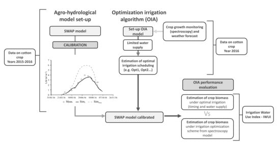
2.7. Evaluation of Different Irrigation Scheduling Approaches through the Simulation Model Application

Once the reliability of the SWAP model had been verified on cotton growth description, the model was applied in the 2016 to evaluate the effect of different irrigation scheduling on crop yield response. In particular, two parameters as efficiency meters for irrigation schedules were used: yield and irrigation water use index (IWUI), which is the ratio between yield and irrigation water supplied during the growing season [57,58]. The latter does not include rainfall, and therefore, is only useful for comparing between nearby fields or farms in the same season.
The applied irrigation scheduling was determined by means (i) SWAP model irrigation scheduling criteria, and (ii) from the weather forecast and field spectroscopy approach.
In the first case, the irrigation water supply was defined by the amount of water to reach field capacity in the root-zone, while the irrigation timing was measured through two different approaches:
(1)
Critical soil pressure head: a combination of two depths (−30 and −40 cm) and two thresholds of soil pressure head (−600 and −800 cm) were applied.
(2)
Allowable daily stress: which is defined by the ratio between the daily actual and potential crop transpiration (Ta Tp−1). In this study, values of ratio were applied from 0.95 to 0.85.
In the second case, the simulation run was performed by applying, as fixed irrigation, the irrigation timing and amount defined by the irrigation optimization approach based on weather forecast and field spectroscopy.

3. Results and Discussion

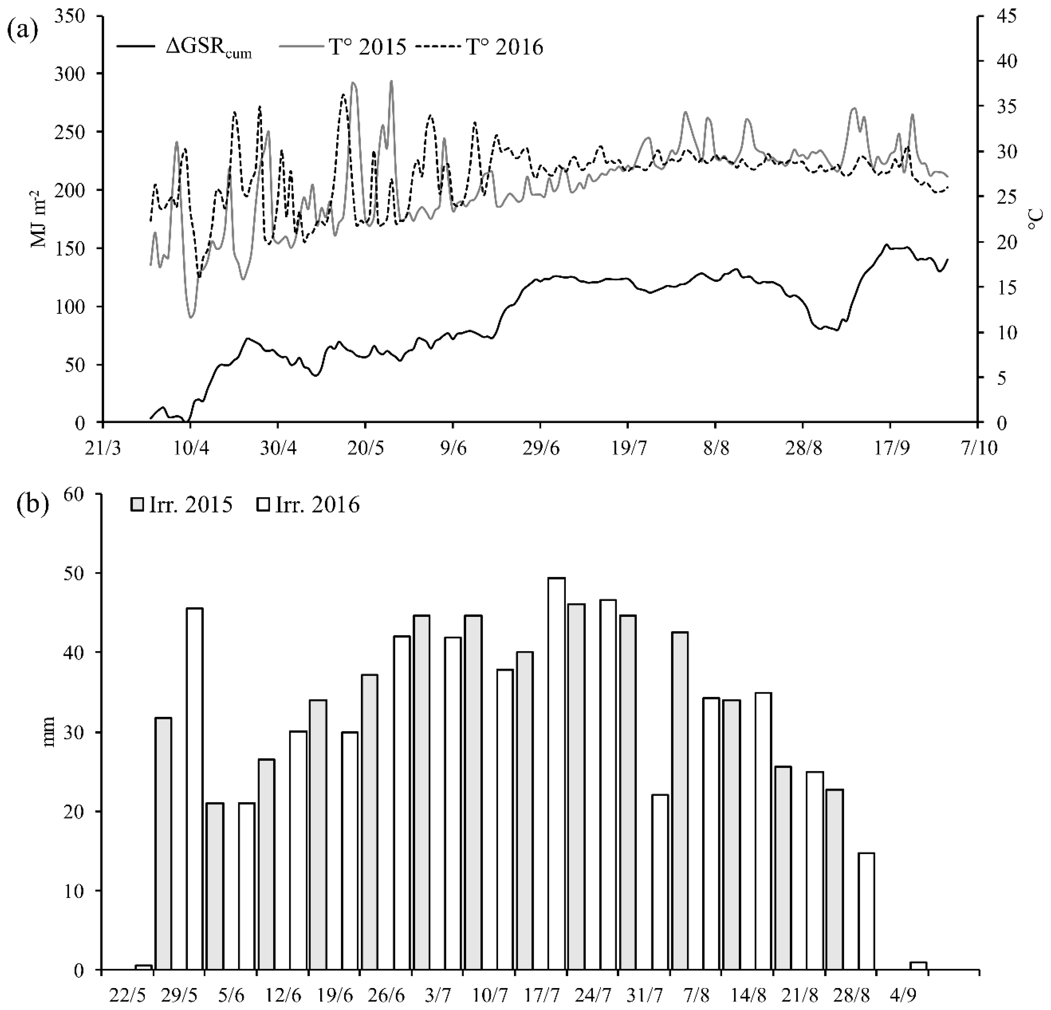
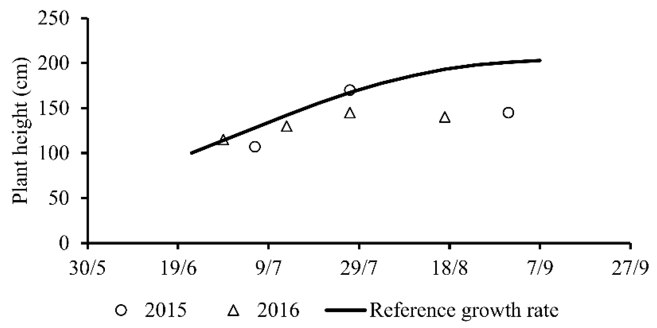
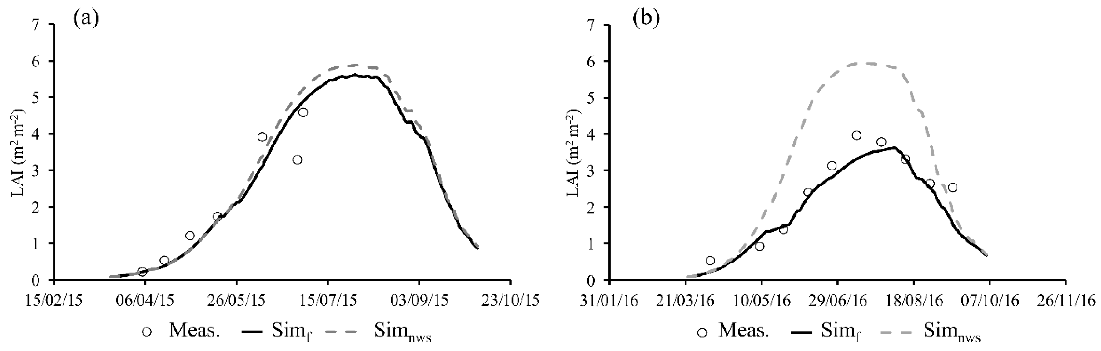
3.1. Cotton Field Results

During both cropping seasons, the cumulative actual ET0 was approximately the same. The summer growing season (March-October) in 2016 was hotter and slightly sunnier than 2015, which is confirmed by differences in cumulative global solar radiation and maximum daily temperatures during cotton growth period (Figure 2a) (Israel Meteorological Service). The seasonal irrigation amount of waters was 4956 m3 ha−1 and 4765 m ha−1 in 2015 and 2016 respectively. The irrigation distribution was different between the years (Figure 2b). Due to lower precipitation in spring 2016, the first watering was more intensive, which caused redistribution of the remaining water during the season.
The irrigation schedule was corrected during the season based on agronomic inspections. The main parameter for correction weekly irrigation water supply was the cotton growth rate (measured crop height was compared with reference values from growth guide [39], Figure 3). The obtained yield was 5.2 t ha−1 in 2015 and 5.1 t ha−1 in 2016, in agreement with a farmer’s expectations (5.5 t ha−1).

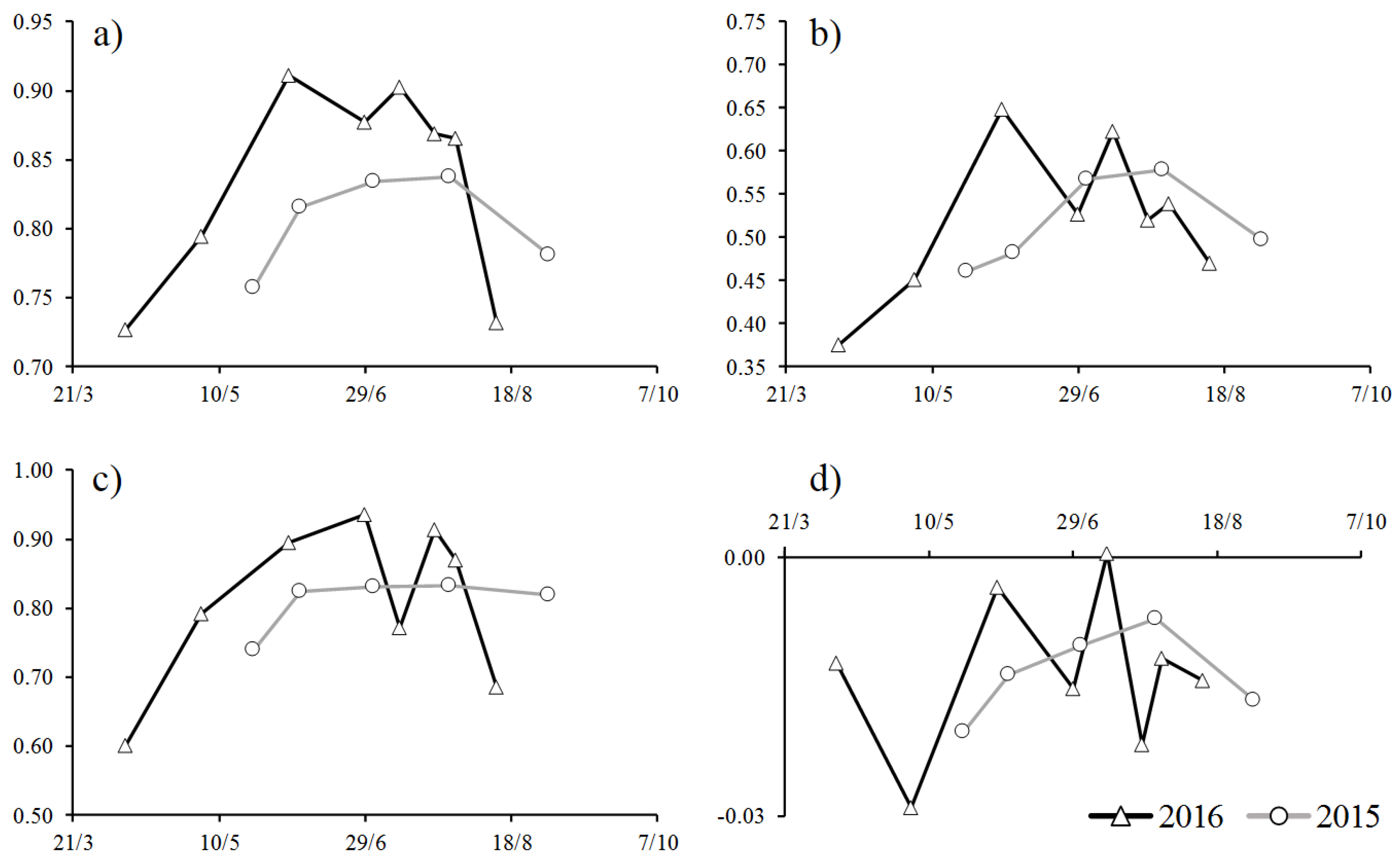
3.2. Cotton State Assessment by Spectroscopy

The agronomic inspections in both growing seasons declare the cotton health state throughout the life cycles. The field spectral observations confirm the results of agronomic inspections. The Vis’ values deviate in the upper bounds; that means high: levels of chlorophyll, green biomass, LAI and photosynthesis rate, according to the original studies (Table 1). However, the temporal graphs (Figure 4) of VIs indicate differences in the two years. In 2015, a stable cotton state was observed during the irrigation period. The minor temporal changes are associated with crop development stages: active growth until the flowering at the end of June leads to an increment in Vis’ values, and slight decreases in VIs since August are associated with fruit formation and ripening. Significantly different from this situation is the VI’s temporal behavior in 2016. The values of the indices were higher at the beginning of the 2016 irrigation period than in 2015. And by the end of June, the values of the indices were significantly reduced and became lower than the corresponding period in 2015 (RENDVI, MCARI2 and PRI). After the regression in NDVI, RENDVI and PRI, in mid-July, there was a restoration of the crop state and an increase in the indices’ values, which again become higher than in 2015. However, at the end of July the decline of those indices repeated, after which cotton health was practically not restored. Such changes in the cotton state resonate with the irrigation schedules. In 2015, there was almost gradual increase in the weekly amount of water until the beginning of July (flowering stage) and then an even more gradual decline until the end of August. It can be assumed that the decrease in the amount of water by June 26, 2015, served as the reason why the values of the indices in early July were slightly lower than at the end of the month. The irrigation schedule in 2016 did not has such gradual behavior. A huge jump can be observed at the beginning of the season, after which the amount of weekly irrigation had low values relative to 2015. In the 2016 irrigation schedule three conspicuous declines could be found: June 5–19, July 10, and July 31. Simultaneously, the decline in the VIs was observed on: June 19, July 23, and August 13. In all three cases, the decline in the values of NDVI, RENDVI and PRI occurred approximately 2 weeks after irrigation decreased. The response of chosen VIs to water state highlights the specificity of cotton growth under limited irrigation. The lower VIs’ results in 2015, exactly identify these conditions, while a large watering level in the beginning of irrigation in 2016 significantly increased the cotton’s health and greenness. Since MCARI2 was related to LAI, it was less sensitive to watering than other indices associated with greenness and health. Similarly, a delayed reaction to changes in the water regime was detected in NDVI, RENDVI and PRI; the decline in MCARI2 on July 11, could mean a reveal of water stress in LAI observed on June 29, by other indices. The more pronounced reaction to irrigation treatments was observed in RENDVI and PRI. RENDVI is a more suitable parameter because all values have a range of 0 to 1, which do not require normalization.

3.3. Definition of Irrigation Scheduling through the Optimization by Weather Forecast and Field Spectroscopy Approach

Developed optimization algorithm was applied to provide an alternative irrigation schedule for a cotton field in 2016. Lower cotton yield and fluctuations in VIs values in the middle of the season highlight imperfections of the irrigation schedule in this year. Effectiveness of the proposed algorithm was assessed by SWAP simulation. Three types of optimized irrigation schedule were introduced to SWAP simulation: by short-term forecast only (Wp1), by matching to the proposed seasonal amount of water (Wp2) and corrected by the field feedback (Wp3). The term (a–b days) for irrigation planning was a week. The excess limit for total amount of water (α) was set at 10%. RENDVI values were used as the field feedback parameter: RENDVI values from cotton spectral measurements in 2015 were used as reference values (Ve) and RENDVI values obtained in 2016 as actual field data (Va). The threshold for index deviation (β) was defined at 15%. In case of significant differences in the values of the reference and actual index values, the irrigation was corrected by γ = 5%. The developed irrigation schedule based on the proposed algorithm is presented on Figure 5.

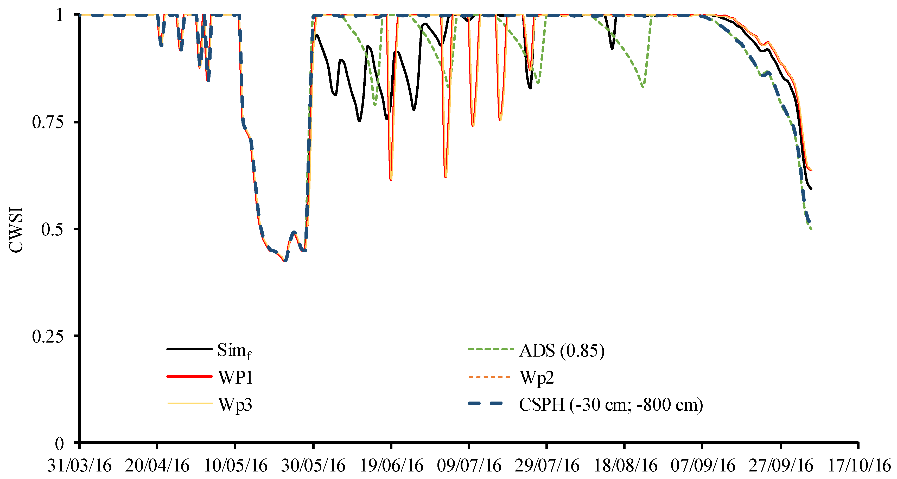
3.4. Cotton Responses to Different Irrigation Schedules

Before, to evaluate the cotton responses under different irrigation scenarios, the simulation model’s performance evaluation was done in both analyzed years (2015 and 2016). The comparison between measured and simulated LAIs showed a good agreement between the data, with the average value of RMSE being 0.53 (±0.17), an EF of 0.68 (±0.01), CRM of 0.03(±0.08) and R of 0.9 (±0.02) (Table 2, Figure 6). Moreover, the yield comparison between measured and simulated LAIs showed an average difference of −0.03% (±0.004) (Table 3).
The efficiency of irrigation schedules considered in this study was assessed by cotton yield and IWUI provided by the simulation model (Table 4). The highest seasonal amount of water was proposed by the first configuration of the proposed algorithm (Wp1), which was performed with no limits for seasonal amount of water and was based on ET0 and Kc only. This configuration leads to lowest IWUI (0.0008 t m−3). It confirms the statement that irrigation planning without an optimization approach leads to low water use efficiency. Application of the irrigation schedule provided by SWAP shows high productivity (IWUI= 0.0011–0.0012 0008 t m−3). The SWAP schedule was designed to meet a soil pressure proposed to be higher, with more water (4761–5285 m3 ha−1), and to provide a higher yield (5.508–5.513 t ha−1). The irrigation developed, taking into account crop water needs through transpiration (allowable daily stress), shows that the same IWUI could be reached with less water (4321–4963 m3 ha−1), which is very important in the regions with limited water supply. The minimal amount of water estimated by SWAP as appropriate for cotton growth (4321 m3 ha−1, when Ta Tp−1 = 0.85) was used for the definition of the seasonal water limit in the proposed optimization algorithm.
The agro-hydrological model allows one to predict water distribution through the soil profile; evaporation; estimated crop water use based on leaf transpiration; and simulate the effect of a lack of water on the cotton growth rate reduction. However, SWAP could not take onto account the non-linear dependency of the cotton productivity from crop water stress at a specific phenological stage (mentioned in Introduction section), since it is not yet described numerically. Therefore, in addition to the absolute values of the cotton yield, the efficiency of seasonal water distribution was evaluated by the occurrence and duration of water shortage through the crop water stress index (CWSI)—ration between Ta Tp−1 (Figure 7).
The first significant water stress was observed in the May, before the irrigation started. In contrast to the SWAP approach and the developed algorithm, the irrigation in practice did not take into account the absence of precipitation in May and did not compensate it. It led to continuous crop stress until the beginning of July, which confirms the LAI rate differences in 2015 and 2016 (Figure 5). Thus, despite the fact that solar radiation in 2016 was higher, which provided a higher potential yield, in fact, the yield was lower than in 2015.
Necessity, permissible limits of stress and their timeliness are factors that are not provided by WOFOST and not considered in the SWAP simulation. Thus, the CSHP approach proposes the highest water consumption, provides conditions without water stress during the irrigation period and consequently provides the highest simulated yield. However, in practice such an approach leads to high plant height and a high number of balls, but low lint yield [36]. The ADS approach allows one to introduce water stress with a defined threshold into irrigation management. It reduces water consumption with minimum yield loss. Nevertheless, this method considers the power of the relationship of yield from water as a constant parameter during the whole growing season as constant, which is not valid in practice [32].
Application the developed optimization algorithm with a limited seasonal amount of water (Wp2 and Wp3) leads to significant (Ta Tp−1 = 0.6) short-term water stresses during cotton development. It ensures that growth restraint subsequently reduces water consumption through transpiration and save more resources for fruit formation. Since SWAP does not simulate this process, it could be assumed that applying this irrigation schedule can provide a higher yield than estimated by the model; i.e., higher IWUI. CWSI doesn’t show differences between Wp2 and Wp3, which confirms once more that SWAP model could not consider completely, crop water stress in the simulation, which was observed on the field by spectrometer.
The results of different optimization scenarios (by SWAP and by the proposed algorithm) shows that strength of each approach depends on the accuracy and completeness of the inputs. In practice the farmers are limited to obtain all required data. Thus, building a model on interchangeable and complementary modules allow to make the it sufficient with limited data and highly-accurate with full input dataset. The main advantage of the optimization by weather forecast and field spectroscopy is introducing accurate field feedback that ensures compliance of the developed schedule with agronomic management principles and prevent critical stresses. The strength part of the SWAP was accurate (simulation of water uptake according to crop development rate and soil characteristics). Integration of the proposed algorithm allows one to take advantage of both methods and vary the configuration of combination both methods according to available inputs and priority tasks (multi-term planning, reducing water costs, maximizing yield etc.).

4. Conclusions

To date, irrigation optimization could be conducted using knowledge from different fields: agronomy, physical modeling and spectral analysis. This study was devoted to highlight benefits and identify gaps of these approaches. Irrigation planning based on agronomic experience considers the specificity of crops’ phenological developments and their effects on yield. Extensive practice allows one to define the optimal time for watering reduction with minimal yield losses. However, this approach does not support quantitative estimation of optimal amount of water and not suited to long-term planning. The simulation models have a number of advantages for agricultural management in general and for irrigation planning in particular. The simulation of crop development under real field conditions, calculation of water balance, long-term planning, and prediction of crop-water needs by short-term and mid-term weather forecasts, can be of significant assistance in making decisions about the amounts of water and the irrigation schedule. Despite that, to the agronomic approach, crop responses to a lack of water at specific phenological stages is not described in agro-hydrological models. Thus, physical modeling allows one to estimate the minimal amount of water for optimal crop growth but is limited by time distribution of water stress. The designed algorithm distributes amount of water, taking into account admissibility of the lack of water at specific phenological stages and the intensity of crop water stress estimated by field spectroscopy. Thus, irrigation scheduling and optimization will be more effective with the use of combined methods: the principles of growth, allowable stresses and crop coefficients provided by crop guides, the estimation of water consumption by a simulation model in common with the weather forecast and feedback from the field such as vegetation indices.

Author Contributions

A.B. (Antonello Bonfante), A.B. (Anna Brook) and M.P. proposed the method, and designed, and performed the experiments; A.B. (Antonello Bonfante), A.B. (Anna Brook), K.S. and M.P. analyzed the data and provided constructive suggestions; M.P. and A.B. (Antonello Bonfante) wrote the paper.

Funding

This work was supported by Israel Water Authority (grant number 41683); and the Israel Innovation Authority, Israel-Italy Joint Innovation Program for Industrial, Scientific and Technological Cooperation (grant number 60283).

Conflicts of Interest

The authors declare no conflict of interest

References

  1. EU Commission. Hard Surfaces Hidden Costs—Searching for Alternatives to Land Take and Soil Sealing; Publications Office of the European Union: Luxembourg, 2013; 31p, ISBN 978-92-79-30550-4. [Google Scholar] [CrossRef]
  2. Nelson, G.C.; Rosegrant, M.W.; Koo, J.; Robertson, R.; Sulser, T.; Zhu, T.; Ringler, C.; Msangi, S.; Palazzo, A.; Batka, M. Climate Change: Impact on Agriculture and Costs of Adaptation; International Food Policy Research Institute: Washington, DC, USA, 2009; Volume 21. [Google Scholar]
  3. Olesen, J.E.; Bindi, M. Consequences of climate change for European agricultural productivity, land use and policy. Eur. J. Agron. 2002, 16, 239–262. [Google Scholar] [CrossRef]
  4. Gornall, J.; Betts, R.; Burke, E.; Clark, R.; Camp, J.; Willett, K.; Wiltshire, A. Implications of climate change for agricultural productivity in the early twenty-first century. Philos. Trans. R. Soc. B-Biol. Sci. 2002, 365, 2973–2989. [Google Scholar] [CrossRef] [PubMed]
  5. Prasad, P.V.V.; Staggenborg, S.A.; Ristic, Z. Impacts of drought and/or heat stress on physiological, developmental, growth, and yield processes of crop plants. In Response of Crops to Limited Water: Understanding and Modeling Water Stress Effects on Plant Growth Processes; Agricultural System Model Series; American Society of Agronomy, Crop Science Society of America, Soil Science Society of America: Madison, WI, USA, 2008; Volume 1, pp. 301–356. [Google Scholar]
  6. Porter, J.R.; Xie, L.; Challinor, A.J.; Cochrane, K.; Howden, S.M.; Iqbal, M.M.; Lobell, D.B.; Travasso, M.I.; Chhetr, N.; Garrett, K.; et al. Climate Change: Impacts, Adaptation, and Vulnerability. In Part A: Global and Sectoral Aspects; IPCC Working Group II; Cambridge Univ. Press: Cambridge, UK, 2014; pp. 485–533. [Google Scholar]
  7. Wilks, D.S.; Wolfe, D.W. Optimal use and economic value of weather forecasts for lettuce irrigation in a humid climate. Agric. For. Meteorol. 1998, 89, 115–129. [Google Scholar] [CrossRef]
  8. Wang, D.; Cai, X. Irrigation scheduling—Role of weather forecasting and farmers’ behavior. J. Water Resour. Plan. Manag. 2009, 135, 364–372. [Google Scholar] [CrossRef]
  9. Allen, R.G.; Pereira, L.S.; Raes, D.; Smith, M. Crop Evapotranspiration-Guidelines for Computing Crop Water Requirements-FAO Irrigation and Drainage Paper 56; FAO: Rome, Italy, 1998; Volume 300, p. D05109. [Google Scholar]
  10. Droogers, P.; Kite, G.; Murray-Rust, H. Use of simulation models to evaluate irrigation performance including water productivity, risk and system analyses. Irrig. Sci. 2000, 19, 139–145. [Google Scholar] [CrossRef]
  11. Geerts, S.; Raes, D. Deficit irrigation as an on-farm strategy to maximize crop water productivity in dry areas. Agric. Water Manag. 2009, 96, 1275–1284. [Google Scholar] [CrossRef] [Green Version]
  12. Smith, M.; Allen, R.; Pereira, L. Revised FAO Methodology for Crop-Water Requirements; 1998 (No. IAEA-TECDOC—1026); International Atomic Energy Agency (IAEA): Vienna, Austria, 1998. [Google Scholar]
  13. O’Toole, J.C.; Cruz, R.T. Response of leaf water potential, stomatal resistance, and leaf rolling to water stress. Plant Physiol. 1980, 65, 428–432. [Google Scholar] [CrossRef] [PubMed]
  14. Thompson, R.B.; Gallardo, M.; Valdez, L.C.; Fernández, M.D. Using plant water status to define threshold values for irrigation management of vegetable crops using soil moisture sensors. Agric. Water Manag. 2007, 88, 147–158. [Google Scholar] [CrossRef]
  15. Basso, B.; Cammarano, D.; De Vita, P. Remotely sensed vegetation indices: Theory and applications for crop management. Ital. J. Agrometeorol. 2004, 53, 36–53. [Google Scholar]
  16. Gamon, J.A.; Penuelas, J.; Field, C.B. A narrow-waveband spectral index that tracks diurnal changes in photosynthetic efficiency. Remote Sens. Environ. 1992, 41, 35–44. [Google Scholar] [CrossRef]
  17. Hernández, E.I.; Melendez-Pastor, I.; Navarro-Pedreño, J.; Gómez, I. Spectral indices for the detection of salinity effects in melon plants. Sci. Agric. 2014, 71, 324–330. [Google Scholar] [CrossRef] [Green Version]
  18. Sims, D.A.; Gamon, J.A. Relationships between leaf pigment content and spectral reflectance across a wide range of species, leaf structures and developmental stages. Remote Sens. Environ. 2002, 81, 337–354. [Google Scholar] [CrossRef]
  19. Priesack, E.; Gayler, S. Agricultural crop models: Concepts of resource acquisition and assimilate partitioning. In Progress in Botany; Springer: Berlin/Heidelberg, Germany, 2009; pp. 195–222. [Google Scholar]
  20. Yin, X.; van Laar, H.H. Crop System Dynamics. An Ecophysiological Simulation Model for Genotype-by-Environment Interactions; Wageningen Academic Publishers: Wageningen, The Neatherlands, 2005; p. 155. ISBN 487063966. [Google Scholar]
  21. Bonfante, A.; Monaco, E.; Manna, P.; De Mascellis, R.; Basile, A.; Buonanno, M.; Cantilena, G.; Esposito, A.; Tedeschi, A.; De Michele, C.; et al. LCIS DSS—An irrigation supporting system for water use efficiency improvement in precision agriculture: A maize case study. Agric. Syst. 2019, 176, 102646. [Google Scholar] [CrossRef]
  22. Hunink, J.; Vila, M.; Baille, A. REDSIM: Approach to Soil WATER modelling. Tools and Data Considerations to Provide Relevant Soil Water Information for Deficit Irrigation; Unpublished Report; FutureWater: Wageningen, The Netherlands, 2011; Volume 32. [Google Scholar]
  23. Terribile, F.; Agrillo, A.; Bonfante, A.; Buscemi, G.; Colandrea, M.; D’Antonio, A.; De Mascellis, R.; De Michele, C.; Langella, G.; Manna, P.; et al. A Web-based spatial decision supporting system for land management and soil conservation. Solid Earth 2015, 6, 903. [Google Scholar] [CrossRef]
  24. Kroes, J.G.; Van Dam, J.C.; Huygen, J.; Vervoort, R.W. User’s Guide of SWAP Version 2.0; Simulation of Water Flow, Solute Transport and Plant Growth in the Soil-Water-Atmosphere-Plant Environment; Wageningen Environmental Research: Wageningen, The Netherlands, 2002; Volume 610, p. 137. [Google Scholar]
  25. Boogaard, H.L.; Van Diepen, C.A.; Rotter, R.P.; Cabrera, J.M.C.A.; Van Laar, H.H. WOFOST 7.1; User’s Guide for the WOFOST 7.1 Crop Growth Simulation Model and WOFOST Control Center 1.5; Wageningen, Winand Staring Centre for Integrated Land, Soil and Water Research: Wageningen, The Netherlands, 1998; Volume 52. [Google Scholar]
  26. Steduto, P.; Hsiao, T.C.; Raes, D.; Fereres, E. AquaCrop—The FAO crop model to simulate yield response to water: I. Concepts and underlying principles. Agron. J. 2009, 101, 426–437. [Google Scholar] [CrossRef]
  27. Todorovic, M.; Albrizio, R.; Zivotic, L.; Saab, M.T.A.; Stöckle, C.; Steduto, P. Assessment of AquaCrop, CropSyst, and WOFOST models in the simulation of sunflower growth under different water regimes. Agron. J. 2009, 101, 509–521. [Google Scholar] [CrossRef]
  28. Eitzinger, J.; Trnka, M.; Hösch, J.; Žalud, Z.; Dubrovský, M. Comparison of CERES, WOFOST and SWAP models in simulating soil water content during growing season under different soil conditions. Ecol. Model. 2004, 171, 223–246. [Google Scholar] [CrossRef]
  29. Dorji, M. Integration of SWAP Model and SEBAL for Evaluation of On-Farm Irrigation Scheduling with Minimum Field Data; ITC: Kolkata, India, 2003. [Google Scholar]
  30. Uran, O.; Janssen, R. Why are spatial decision support systems not used? Some experiences from the Netherlands. Comput. Environ. Urban Syst. 2003, 27, 511–526. [Google Scholar] [CrossRef]
  31. Wenkel, K.O.; Berg, M.; Mirschel, W.; Wieland, R.; Nendel, C.; Köstner, B. LandCaRe DSS–An interactive decision support system for climate change impact assessment and the analysis of potential agricultural land use adaptation strategies. J. Environ. Manag. 2013, 127, S168–S183. [Google Scholar] [CrossRef]
  32. Kirda, C. Deficit Irrigation Scheduling Based on Plant Growth Stages Showing Water Stress Tolerance; Deficit Irrigation Practices, Water Reports; Food and Agricultural Organization of the United Nations: Rome, Italy, 2002; Volume 22. [Google Scholar]
  33. Bauer, P.; Faircloth, W.; Rowland, D.; Ritchie, G.; Perry, C.; Barnes, E. Water-sensitivity of cotton growth stages. In Cotton Irrigation Management of Humid Regions, Cotton Incorporated; University of Georgia: Athens, Greece, 2012; pp. 17–20. [Google Scholar]
  34. Cakir, R. Effect of water stress at different development stages on vegetative and reproductive growth of corn. Field Crops Res. 2004, 89, 1–16. [Google Scholar] [CrossRef]
  35. Ghobadi, M.; Bakhshandeh, M.; Fathi, G.; Gharineh, M.H.; Alami-Said, K.; Naderi, A.; Ghobadi, M.E. Short and long periods of water stress during different growth stages of canola (Brassica napus L.): Effect on yield, yield components, seed oil and protein contents. J. Agron. 2006, 5, 336–341. [Google Scholar]
  36. Karam, F.; Lahoud, R.; Masaad, R.; Daccache, A.; Mounzer, O.; Rouphael, Y. Water use and lint yield response of drip irrigated cotton to the length of irrigation season. Agric. Water Manag. 2006, 85, 287–295. [Google Scholar] [CrossRef]
  37. USDA-Natural Resources Conservation Service. Soil Survey Staff. Keys to Soil Taxonomy, 12th ed.; USDA-Natural Resources Conservation Service: Washington, DC, USA, 2014. [Google Scholar]
  38. Eswaran, H.; Cook, T. Classification and Management-related Properties of Vertisols. In Management of Vertisols in Sub Saharan Africa, Proceeding of the Conference Held at ILCA, Addis Ababa, Ethiopia, 31 August–4 September 1987; ILCA: Addis Ababa, Ethiopia, 1988; pp. 64–85. [Google Scholar]
  39. ADAMA Agan Ltd. Cotton Growth Management 2014–2015; ADAMA Agan, Ltd.: Ashdod, Israel, 2014. [Google Scholar]
  40. Jackson, R.D.; Clarke, T.R.; Moran, M.S. Bidirectional calibration results for 11 Spectralon and 16 BaSO4 reference reflectance panels. Remote Sens. Environ. 1992, 40, 231–239. [Google Scholar] [CrossRef]
  41. Jones, H.G. Irrigation scheduling: Advantages and pitfalls of plant-based methods. J. Exp. Bot. 2004, 55, 2427–2436. [Google Scholar] [CrossRef] [PubMed]
  42. Basso, B.; Cammarano, D.; Carfagna, E. Review of crop yield forecasting methods and early warning systems. In Proceedings of the First Meeting of the Scientific Advisory Committee of the Global Strategy to Improve Agricultural and Rural Statistics, FAO Headquarters, Rome, Italy, 18–19 July 2013. [Google Scholar]
  43. Li, H.; Zheng, L.; Lei, Y.; Li, C.; Liu, Z.; Zhang, S. Estimation of water consumption and crop water productivity of winter wheat in North China Plain using remote sensing technology. Agric. Water Manag. 2008, 95, 1271–1278. [Google Scholar] [CrossRef]
  44. Ranjan, R. Identification and Differentiation of Water and Nitrogen Stresses Using Hyperspectral Remote Sensing. Ph.D. Thesis, Iari, Division of Agricultural Physics, New Delhi, India, 2012. [Google Scholar]
  45. Van Beek, J.; Tits, L.; Somers, B.; Coppin, P. Stem water potential monitoring in pear orchards through WorldView-2 multispectral imagery. Remote Sens. 2013, 5, 6647–6666. [Google Scholar] [CrossRef]
  46. Rouse, J., Jr.; Haas, R.H.; Schell, J.A.; Deering, D.W. Monitoring Vegetation Systems in the Great Plains with ERTS. In Goddard Space Flight Center 3d ERTS-1 Symp. Vol. 1, Sect. A; NASA Goddard Space Flight Center: College Station, TX, USA, January 1974; pp. 309–317. [Google Scholar]
  47. Haboudane, D.; Miller, J.R.; Pattey, E.; Zarco-Tejada, P.J.; Strachan, I.B. Hyperspectral vegetation indices and novel algorithms for predicting green LAI of crop canopies: Modeling and validation in the context of precision agriculture. Remote Sens. Environ. 2004, 90, 337–352. [Google Scholar] [CrossRef]
  48. Penuelas, J.; Filella, I.; Gamon, J.A. Assessment of photosynthetic radiation-use efficiency with spectral reflectance. New Phytol. 1995, 131, 291–296. [Google Scholar] [CrossRef]
  49. Van Genuchten, M.T. A closed-form equation for predicting the hydraulic conductivity of unsaturated soils. Soil Sci. Soc. Am. J. 1980, 44, 892–898. [Google Scholar] [CrossRef]
  50. Mualem, Y. A new model for predicting the hydraulic conductivity of unsaturated porous media. Water Resour. Res. 1976, 12, 513–522. [Google Scholar] [CrossRef] [Green Version]
  51. Ritchie, J.T. Model for predicting evaporation from a row crop with incomplete cover. Water Resour. Res. 1972, 8, 1204–1213. [Google Scholar] [CrossRef] [Green Version]
  52. Feddes, R.A.; Kowalik, P.J.; Zaradny, H. Simulation of Field Water Use and Crop Yield; Wageningen Centre for Agricultural Publishing and Documentation: Wageningen, The Netherlands, 1978. [Google Scholar]
  53. Hijmans, R.J.; Guiking-Lens, I.M.; Van Diepen, C.A. WOFOST 6.0: User’s Guide for the WOFOST 6.0 Crop Growth Simulation Model; Winand Staring Centre for Integrated Land, Soil and Water Research: Wageningen, The Netherlands, 1994; Volume 12. [Google Scholar]
  54. Loague, K.; Green, R.E. Statistical and graphical methods for evaluating solute transport models: Overview and application. J. Contam. Hydrol. 1991, 7, 51–73. [Google Scholar] [CrossRef]
  55. Greenwood, D.J.; Neeteson, J.J.; Draycott, A. Response of potatoes to N fertilizer: Dynamic model. Plant Soil 1985, 85, 185–203. [Google Scholar] [CrossRef]
  56. Addiscott, T.M.; Whitmore, A.P. Computer simulation of changes in soil mineral nitrogen and crop nitrogen during autumn, winter and spring. J. Agric. Sci. UK 1987, 109, 141–157. [Google Scholar] [CrossRef]
  57. Skewes, M. Irrigation Benchmarks and Best Management Practices for Winegrapes; Primary Industries and Resources SA: Adelaide, Australia, 1997. [Google Scholar]
  58. Purcell, B.; Associates Pty Ltd. Determining a Framework, Terms and Definitions for Water Use Efficiency in Irrigation [R/OL]; Report to Land and Water Resources Research and Development Corporation; Consulting Water Resources and Irrigation Engineers: Narrabri, Australia, 1999. [Google Scholar]
Figure 1. Algorithm for the irrigation optimization schedule by weather forecast and field spectroscopy.
Remotesensing 11 02127 g001
Figure 2. In the above panels are reported: (a) the difference between cumulative global solar radiation in 2016 and 2015 (ΔGRScum); daily maximal temperature in 2015 (T° 2015) and 2016 (T° 2016); (b) weekly irrigation amount during both crop growing seasons (Irr.2015 and Irr.2016).
Remotesensing 11 02127 g002
Figure 3. Cotton height after the flowering stages in 2015 and 2016 (dots and triangles) compared to the reference growth rate [38].
Remotesensing 11 02127 g003
Figure 4. Temporal behavior of vegetation indices obtained in 2015 and 2016 from the cotton field: (a) NDVI; (b) RENDVI; (c) MCARI2; (d) PRI.
Remotesensing 11 02127 g004
Figure 5. Irrigation schedule developed based on the proposed optimization algorithm in comparison with actual irrigation on cotton field in 2016.
Remotesensing 11 02127 g005
Figure 6. Measured (Meas.) and simulated leaf area index (LAI) of cotton (under field conditions—Simf, and without water stress—Simnws) during the years: (a) 2015 and (b) 2016.
Remotesensing 11 02127 g006
Figure 7. Crop water stress index response to the irrigation schedules developed by different approaches: Simf—agronomic management; CSPH—critical soil pressure head (−800 cm at soil depth −30 cm); Wp1, Wp2 and Wp3—optimization by weather forecast and field spectroscopy.
Remotesensing 11 02127 g007
Table 1. Vegetation indexes applied in this study.
VIType of SensitivityFormula for Spectrometer DataRange of ValuesReference
NDVIGreen biomass ( w 800 w 670 ) ( w 800 + w 670 ) 0 to 1[46]
RENDVIChlorophyll level ( w 750 w 705 ) ( w 750 + w 705 ) 0.2 to 0.9[18]
MCARI2Leaf Area Index 1.5 ( 2.5 ( w 800 w 670 ) 1.3 ( w 800 w 550 ) ) ( 2 w 800 + 1 ) 2 ( 6 w 800 5 w 670 ) 0.5 ) 0 to 1[47]
PRIPhotosynthetic Radiation Use Efficiency ( w 531 w 570 ) ( w 531 + w 570 ) −1 to 1[48]
Table 2. Evaluation of simulation of crop growth performance.
Statistical IndexesLAI (m2 m−2)
20152016
RMSE0.650.41
EF0.690.67
CRM−0.030.09
r0.880.91
Table 3. Measured (Meas.) and simulated cotton yield under field condition (Simf) and without water stress (Simnws) in the years 2015 and 2016.
YearMeas.SimfSimnws
(kg ha−1)
2015520051835445
2016510051145517
Table 4. Crop responses to different irrigation criteria in 2016 obtained from simulation runs.
Irrigation CriteriaIrrigation (m3 ha−1)Yield (t ha−1) IWUI (t m−3)
Critical Pressure head
Soil depthSoil Pressure head
−30 cm−600 cm52855.5130.0010
−30 cm−800 cm47615.5080.0012
−40 cm−600 cm52185.5120.0011
−40 cm−800 cm49055.5070.0011
Allowable Daily stress
Ta Tp−10.9549635.3910.0011
0.9047465.2590.0011
0.8543215.1220.0012
0.8044484.9680.0011
Optimization algorithm
Wp164314.8300.0008
Wp241314.9750.0012
Wp341564.9390.0012
Real field conditions47665.1140.0011
IWUI = Irrigation Water Use Index.

