Abstract
Airborne laser scanning (ALS) and digital aerial photogrammetry (DAP) have both been demonstrated as reliable sources of information on forest stand inventory attributes. The increasing availability of both datasets provides a means for improving stand dynamics information over time; however, the cost of multi-temporal ALS can be prohibitive in some circumstances. As a result, a combination of ALS at an initial time step and subsequent updates using DAP has been proposed as a cost-effective alternative for maintaining forest inventories. In this study we used low density ALS and DAP point clouds acquired in 2007 and 2015, respectively, to quantify changes in forest structure, in a highly disturbed boreal mixedwood forest in Alberta, Canada. We examined the capacity of the two technologies to model changes in top height (H), volume (V), and basal area (BA) using both direct and indirect approaches for estimation. Results indicate that the proportion of explained variance (adjusted R2) for the models derived from the ALS (Time 1; T1) and DAP (Time 2; T2) data were highest for models predicting H at T1, and lowest for BA at T1 and T2 (R2 was 0.66–0.70). The indirect estimates of change in H, BA, and V were calculated by subtracting the T1 and T2 predictions. For the direct approach, separate regression models were developed that used the differences in point cloud metrics between T1 and T2 as predictors. Results indicated that the accuracy of the estimates generated using the indirect approach were markedly lower than the estimates generated using the direct approach, with especially poor results for ∆BA and ∆V. Best results were achieved for ∆H using the direct approach with an R2 coefficient of 0.65 and an root mean square error (RMSE)% of 190.06%. We found that the error associated with change estimates of H, BA and V increased with the increase or decrease in mortality. We conclude that forest managers should act carefully when applying the multi-temporal and multi-sensor analysis of forest growth if forest growth is slow and the level of mortality is high.
1. Introduction
Canadian boreal forests and woodlands cover approximately 347 Mha [1] making up nearly 10% of forest cover globally. As a result, sustainable forest management strategies for timber production and ecosystem services including carbon sequestration, clean water production, and biodiversity conservation are critically important [2]. One key component of sustainable forest management is the timely and accurate acquisition of forest information to quantify the amount and condition of forest resources. This includes the evaluation of structural change over time, which can inform growth models critical for developing future predictions of forest inventory variables [3]. To date, forest inventory methods have focused on ground-based measurements, complemented with the manual interpretation of aerial photography for stand delineation, species identification, and structural quantification [4].
The development and implementation of three-dimensional point cloud datasets acquired with airborne platforms to measure forest stand inventory attributes have become the basis of precision forestry [5] and have been deemed promising as cost-effective and spatially extensive means of supplementing the current modes of inventory using the area-based approach (ABA) [6]. Two common methods may be used in developing the required point clouds: (1) Airborne laser scanning (ALS) technologies, which measure the time between emitted sensor pulses and received reflections [7]; and (2) digital aerial photogrammetry (DAP) which produces image-based outputs by matching points on stereo aerial photographs and calculating the parallax [8]. While the concepts of ALS are well known, the basis of DAP involves deriving the measurement of an object’s position based on images acquired from two or more locations. A digital surface model (DSM) can be created when this method is applied on multiple overlapping images [9]. Image acquisition flights are usually performed higher and faster than ALS flights. With a wider field of view, image platforms are able to cover a much larger area for a given amount of flying hours. Overall, image acquisition is estimated to cost one-half to one-third to that of ALS data [8]. However, image-matching algorithms are only successful when objects are directly visible in the images themselves. Without penetrability, image-based point clouds can solely explain upper canopy structure [10]. To normalize the returns to elevations above terrain, an external terrain model is required, preferably derived from ALS data [11], particularly beneath forest canopies. Imagery is also influenced by brightness and viewing angles, which limit optimal flying hours [7,8]. While ALS data can produce highly accurate vegetation profiles, repeated acquisitions for growth monitoring only from ALS can be costly and often involve trade-offs between the area covered and issues such as point density and scan angle [12]. As a result, a combination of the two technologies, with ALS as the initial measurement followed by updates of DAP, is seen as an optimal solution to obtain forest growth estimates over large spatial extents.
Boreal forests can have heterogeneous patterns of composition and structure and are driven by different disturbance agents, particularly wildfire [13]. Boreal forests in Canada are dominated by several genera including Abies, Betula, Larix, Picea, Pinus and Populus, with varying growth rates between regions [14,15,16]. Slow growth can be difficult to correctly quantify in the field if growth changes are small compared to instrument errors [17]. In addition, the cost of locating and measuring the required number of field plots logistically limits data collection spatially and temporally, especially in remote areas.
Several studies have investigated the use of multi-temporal point cloud datasets to monitor forest growth. St-Onge and Vepakomma [18] evaluated the height growth in hardwood and softwood stands and by three height classes. They showed that the average differences in the upper height percentiles were near to the average observed growth in deciduous and coniferous stands. The increment in height was generally close to the reference age–height table values (average deviation = 0.42 m). Næsset and Gobakken [19] measured growth at plot and stand levels in Lorey’s height (HL). Their results showed that the increment in height was often close to the root mean square error (RMSE), indicating challenges related to the use of point cloud datasets, especially in the young stands. HL growth was also analyzed by Hopkinson et al. [20], who showed that DSM-based height growth estimates were nearly parallel to the reference. Yu et al. [21] demonstrated three methods to estimate HL growth: individual tree crown differencing, DSM differencing, and an ABA. The ABA yielded the least accurate results, with the lowest R2 value and the highest RMSE. As shown by Véga and St-Onge [22], longer time intervals between data acquisitions increase the accuracy of height growth despite errors in in height estimates at individual times. Estimates of stand growth can also be calculated by integrating exisitng growth simulators with ALS or DAP-based predictions of forest attributes [23,24]. Cell-level yield curves can be computed by assigning weights to the input attributes based on their prediction accuracy.
Overall, studies assessing growth with multi-temporal remotely sensed data have been more successful in forests with taller mean stand heights. Growth assessments in temperate forest zones have usually been more successful, though assessments from boreal forest zones have varied. In boreal studies, success was caused by using large growth intervals [22] and comparatively simpler stand structures [21]. No patterns of successful outcomes to growth assessments were apparent regarding scale or sensor choice. Few studies that have evaluated height growth have validated their models against independent data sources, and only two have utilized a multi-sensor method [22,24]. A multi-sensor method can reduce the expense of obtaining multi-temporal point cloud data for stand-level growth evaluations. It does so by leveraging the ALS-derived digital terrain model (DTM) from an initial acquisition of ALS data for the subsequent processing of DAP data acquisitions [8].
In this study, we examined the capacity of ALS and DAP technologies to assess the change in top height (∆H), change in basal area per ha (∆BA), and change in total volume per ha (∆V) over roughly eight years in managed yet highly disturbed boreal forest stands near Slave Lake in central Alberta, Canada. Through this analysis, we asked the following specific questions.
What is the predictive capability of integrated ALS and DAP technologies to quantify ∆H, ∆BA, and ∆V?
The majority of existing studies that used a bi-temporal point cloud to characterize stand growth have used ALS data [18,19,20,21] or relied on dense DAP point clouds [25]. Because of the differences between ALS and DAP point clouds, additional research is required to analyze the specific aspects of combining these datasets for quantifying change in stand conditions.
Which modeling approach (direct or indirect) provides more accurate estimates of ∆H, ∆BA, and ∆V, when ALS- and DAP-based predictors are used?
The change in forest attributes can be estimated either directly (i.e., a single model is developed to predict change) or indirectly (i.e., based on a difference between two separate models developed to predict values at Time 1 (T1) and Time 2 (T2)) [26,27]. It is unclear which of these two approaches is better suited for characterizing change in forest attributes when low density ALS and DAP point clouds are used and when the forest growth is slow.
How is the predictive capability for ∆H, ∆BA, and ∆V impacted by increasing plot-level mortality?
Stand-level mortality has been shown to alter forest structure [28]. Existing approaches to quantify mortality using point cloud datasets utilize return intensity-based metrics as predictors [29,30]. However, intensity metrics from ALS data are often not calibrated and vary due to differences in acquisition parameters. In the absence of a method to enumerate mortality directly from the point cloud data, there is a need to measure the impacts of plot-level mortality on the accuracy of area-based estimates of forest attributes. To assess the impacts of plot-level mortality on ∆H, ∆BA, and ∆V estimates in Slave Lake, we iteratively measured the accuracy of optimized height models while incrementing the number of plots with mortality in the dataset.
2. Materials and Methods
2.1. Study Area
The Slave Lake Forest Management Area covers approximately 700,000 ha and is located near the township of Slave Lake, Alberta (Figure 1). The study area is situated in the Central Mixedwood, Lower Foothills, and Upper Foothills natural subregions. The annual precipitation is 600 mm, while the mean summer and winter temperatures are 20 and −21 °C, respectively [31]. The elevation ranges from 546 to 1375 m a.s.l. The Slave Lake forest is a mixedwood boreal stand including aspen (Populus tremuloides), white spruce (Picea glauca), balsam poplar (Populus balsamifera), Lodgepole pine (Pinus contorta) and black spruce (Picea mariana) as some of the most common species [31].
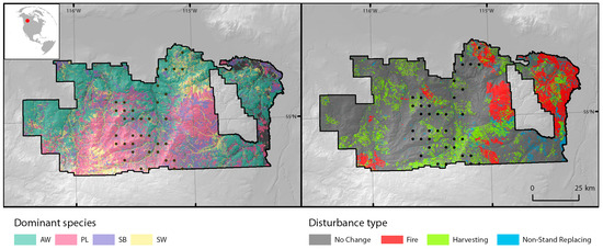
Figure 1.
Location and outline of the study area. Black dots indicate sample plot locations. Dominant species codes: AW: Trembling aspen; PL: Lodgepole pine; SB: Black spruce; SW: White spruce.
Forest dynamics in the region are characterized by natural and anthropogenic disturbances including wildfires, harvesting activities, oil and gas exploration, and non-stand replacing disturbances such as wind damage (Figure 1). A large fire occurred in 2011 that burned 40% of the township.
2.2. Ground Plot Measurements
Thirty-eight plots were established and monitored between 2004 and 2006, and they were re-measured in 2012, 2016 or 2018. The circular plots each had a radius of 11.28 m (400 m2). For every tree in the plot, we measured the location, species, diameter at breast height (DBH), height, height-to-live-crown, and crown class (dominant, codominant, intermediate or suppressed). Plot-level summaries of individual tree measurements included top height (H), basal area (BA), total volume (V). Only trees with a DBH over 7 cm were measured. Plots were omitted if they had mortality rates of 100% or if there was evidence of harvesting, fire or significant blowdown within the plot during the measurement period. Standing dead trees were measured and included in the analysis of mortality. Plot-level summaries were projected from the year they were collected to the year of the ALS or DAP data acquisition. Projections were performed with GYPSY (Growth and Yield Projection System), which is a forest stand-based growth simulator developed by the Alberta Agriculture and Forestry Ministry of the Government of Alberta, Canada [32]. ∆H, ∆BA, and ∆V were calculated as the difference between the projected T1 and T2 values for a plot. The projected plot-level data are summarized in Table 1.

Table 1.
Summary of the ground plot data.
2.3. ALS Data
ALS data were acquired for the study area between 2006 and 2008. The point clouds were collected with an Optech ALTM 3100 sensor. Very similar flight and acquisition parameters were used in all cases, with a scan angle of 50°, a flight speed of 160 kts, and a flying height between 1250 and 1400 m. The average point density was 1.5 pts/m2.
2.4. DAP Data
A total of 1527 aerial images were acquired on 26 April, 9 May and 13 May 2015 using a Z/I DMC II230 at nadir including blue, green, red and near-infrared spectral bands. The ground sample distance was 0.3 m, and the along-track and across-track overlaps were 60% and 30%, respectively. One hundred and thirty-four ground control points were used to register the data.
The DAP data were processed using the Agisoft PhotoScan software. The software first detected points in the source photos that were stable under viewpoint and lighting variations and generated a descriptor for each point based on its local neighborhood. It then used a greedy algorithm to find approximate camera locations and refined them later using a bundle-adjustment algorithm similar to Bundler [33]. A surface was then constructed using the pair-wise depth map computation [34] and blended with the source images to form a texture atlas. This resulted in a point cloud with an average point density of 0.82 points/m2.
As DAP point clouds are known to exhibit systematic distortions relative to absolute coordinate systems, especially in the vertical direction, largely due to radial distortion [35], an additional point cloud post-processing procedure was used for DAP processing. This procedure aimed to correct offsets between an imprecise DAP point cloud known to contain distortion and a precisely georeferenced reference ALS point cloud. We used the iterative closest point (ICP) algorithm, well-known to be effective in point cloud registration [36,37,38], to generate a series of estimated vertical shifts across the study area. To gather the shift observations, the ICP algorithm was applied to raw ALS and DAP point clouds at each increment of a moving window operation with widths of 50 and 150 m between windows. Values produced by the ICP estimation, stored as points at each window centre, include X, Y and Z translation vectors, a rotation matrix, and the root-mean-square error (RMSE) between the resulting aligned point clouds. These results were filtered for noise based on manually adjusted quantile thresholds. Additionally, the point estimates were masked by roads and recently harvested stands to ensure ground-to-ground matching. A polynomial model was developed to estimate vertical shifts (Zshiftxy) in two-dimensional space such that:
where is the x-coordinate, is the y-coordinate, and β0, …, βn are coefficients of the polynomial model. Polynomial orders of up to 20 were tested for both and to acquire the model with the best fit, which was then used to adjust the raw DAP point cloud elevation values based on the predicted vertical shifts.
2.5. Point Cloud Data Processing
The point clouds were processed following standard processing routines, which included tiling, ground classification (ALS data only), and height normalization. A DTM was developed using ground-classified returns from the ALS dataset at a 2 m spatial resolution. The DTM was then used to normalize both the ALS and DAP point heights. Studies have shown that ALS can accurately and precisely be used to normalize DAP point clouds, assuming the ground is stationary between fly-overs [9].
Statistical metrics describing forest stand structure were extracted from the ALS and DAP point clouds within the sample plots. Metrics were generated using returns above 2 m [39] and using only first returns in case of the ALS. Metrics included measures of central tendency (mean, median, mode), measures of dispersion (variance, standard deviation, interquartile range), percentiles, proportions, and densities of point heights above ground. All metrics were calculated using the lidR package for R [40,41].
2.6. Predictive Models
Ordinary least squares (OLS) regression was used to estimate H, BA, and V from ALS data at T1 and DAP data at T2. A stepwise variable selection approach was used to develop a total of six regression models. Models for H were based on a single ALS- or DAP-based predictor describing canopy height. Models of BA, and V used a maximum of four variables following the approach of Bouvier et al. [42]. Predictor variables were selected to characterize stand height, heterogeneity of stand height, canopy cover, and stand vertical complexity. We tested different combinations of variables from each of these groups, as well as different variable transformations, selecting a final model based on the AIC coefficient. We calculated the bias and RMSE (absolute and relative) and used an equivalence test to assess the predictions. Specifically, we used the equiv.boot function available in the equivalence package for R [43] to validate the models. In this regression-based test of equivalence, a linear regression model is established between the observations and predictions, and predetermined regions of equivalence are established for the intercept and slope. The tests for intercept and slope are performed independently and are based on determining if the confidence intervals are contained inside the regions of equivalence [44]. As described by Fekety et al. [45], the test for intercept informs on the bias and determines if the means of the two compared variables are equal. The test for slope, which determines if the slope is equal to 1, informs on the proportionality of the observed and predicted variables. We used the default region of equivalence of ±25%, as per previous studies [45,46,47].
Two methods are commonly applied to evaluate forest growth using three-dimensional point cloud datasets: Direct and indirect methods [26,27]. Direct methods estimate growth from differences in common metrics acquired from two datasets from two different points in time. Indirect methods calculate growth by differencing two independent estimates, at T1 and T2, with the two models not requiring the same predictor variables [48]. We applied both methods to test their feasibility for estimating stand growth. In the indirect approach, the predicted values for ∆HI, ∆BAI, and ∆VI were derived by differencing the predicted values from models at T1 and T2. To apply the direct approach, we first calculated differences between point cloud metrics derived for T1 and T2. These difference metrics were then used as candidate predictors in OLS models to estimate ∆HD, ∆BAD, and ∆VD.
Relative bias, absolute bias and RMSE were calculated as follows:
where N is the number of plots, yi is the observed value at plot i, ŷi is the predicted value at plot i, and ȳ is the mean of the observed variable over all plots.
The RMSE values for ∆HI, ∆BAI, and ∆VI (indirect approach) were calculated from the RMSEs for the models at times T1 and T2 as per Equation (6) adapted from [49]:
where RMSEG is the root mean square error of the growth model and RMSET1 and RMSET2 are the errors of the T1 and T2 models. The predictions of growth were also assessed using the equivalence test as described above.
2.7. Sensitivity of Model Outcomes to Plot-Level Mortality
To observe the impact of tree mortality on the model predictions, we analyzed how the RMSE% changes with different levels of stand-level mortality. To do that, we developed indirect and direct models for ∆H, ∆BA, and ∆V iteratively, using a subset of plots for each iteration. The number of plots increased at each iteration, and by ordering the plots by the level of mortality, the accuracy of each model could be related to the level of plot mortality. At each iteration, predictions and RMSEs were generated from the separate T1 and T2 models (indirect approach) and from a single model for the direct approach.
Mortality was defined as the change in percentage of dead trees basal area in a plot between T1 and T2, and it was calculated as follows:
where BAall is the total basal area of a plot and BAdead is basal area of dead trees.
3. Results
3.1. Plot-Level Estimates of Forest Attributes
The proportion of explained variance (adjusted R2) for the models derived from the ALS (T1) and DAP (T2) data were highest for models predicting HT1 and lowest for BAT1, BAT2, and BAT1, for which the R2 was 0.66–0.70 (Figure 2, Table 2). A power regression approach was used for modeling BA and V, and a bias correction factor was used when back-transforming the predicted values. The highest RMSE% was for VT1 (40.1%). The correlation coefficients between independent variables were always lower than 0.7 for models with more than one independent variable. All independent variables remaining in each of the models were significant (α = 0.05). The results of the equivalence test (Figure 3) showed that the predictions of all attributes were statistically equivalent in terms of bias and that predictions of HT1, HT2 and BAT1 were statistically equivalent in terms of proportionality.
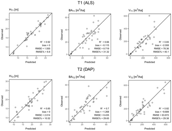
Figure 2.
Observed vs predicted values for the three modeled stand attributes: Top height (H), basal area (BA), and total volume (V). Stand attributes modeled using airborne laser scanning (ALS) data at Time 1 (T1) and digital aerial photogrammetry (DAP) data at Time 2 (T2).
Table 2.
Predictive models for top height (H), basal area (BA), total plot volume (V). Dependent variables denoted with T1 were modeled using ALS data acquired at T1 (2006–2008), while T2 variables were modeled using DAP data from T2 (2015). Predictor variables used in these models included the 20th percentile of point heights (P20), the 95th percentile of point heights (P95), the proportion of points above 5 m (PERC_ABOVE_5), the standard deviation of point heights (SD), and the kurtosis of point heights (KURT).
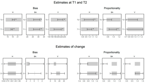
Figure 3.
Results of bootstrapped equivalence tests for stand attributes modeled at T1 and T2 (top) and change estimated with the indirect (I) and direct (D) approach (bottom). In each case, the equivalence test is performed for bias and for proportionality. The grey rectangle indicates the region of equivalence, while the black crossbar depicts the 95% confidence interval. An asterisk indicates cases when the test is satisfied (i.e., confidence interval within the region of equivalence).
3.2. Indirect and Direct Estimates of Change in Forest Attributes
Results for both the direct and indirect approaches to estimating growth are presented in Figure 4 while model forms for ∆HD, ∆BAD, and ∆VD are presented in Table 3. Results showed that the accuracy of the change models was markedly lower when compared to the accuracy of individual models of H, BA, or V using T1 or T2 data. Results also showed that the indirect approach was less accurate than the direct approach in all of the cases, with especially poor results for ∆BAI and ∆VI. Results were best for ∆H when the direct approach was used (∆HD). Under this approach, the R2 coefficient was 0.65 and the RMSE% of 190.06% was lowest across all modeled variables and approaches. The accuracy of ∆HI was lower, with an R2 of 0.42 and an RMSE% of 251.59%. ∆BAD and ∆VD had R2 values of 0.35 and 0.39, respectively; however, extreme values of RMSE% were observed for ∆BAD. The results of the equivalence test (Figure 3) showed that the predictions of change were not statistically equivalent in any of the variables or approaches.
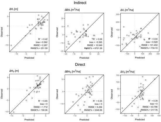
Figure 4.
Scatterplots of the observed versus predicted values for change in top height (H), basal area (BA), and volume (V) using the indirect and direct approaches.
Table 3.
Predictive models for change in top height (∆HD), change in basal area (∆BAD), and change in total volume (∆VD) under the direct approach. Predictor variables used in these models included the change in 99th percentile of point heights (∆P99), the change in proportion of points above 2 m (∆PERC_ABOVE_2), and the change in standard deviation of point heights (∆SD).
3.3. Influence of Stand Mortality on Change Prediction Accuracy
We found that the error associated with estimates of ∆H, ∆BA, and ∆V increased with increasing absolute plot-level mortality. For all three attributes, the RMSE% increased markedly when the mortality increased or decreased (Figure 5). The positive values of mortality indicate the increase in proportion of dead trees basal area between T1 and T2, while a mortality value below 0 indicates ingrowth—new trees growing into the minimum measurable size during the measurement period or that the dead trees were no longer present in the stand. As the direct approach showed to be more accurate in predicting change in stand attributes (Figure 4), for similar values of mortality, the RMSE% values were also lower for the direct approach. Results show that for ∆HD a mortality of about 18% corresponded to a 100% RMSE% value and that value doubled when mortality is close to 30%. For ∆V, results were similar, although a mortality level at 20% corresponded to a higher RMSE% of about 200%. Though the pattern on the relationship between mortality and RMSE% was similar for ∆BA, RMSE% reached extreme values that resulted from the poor accuracy, especially of the indirect model.
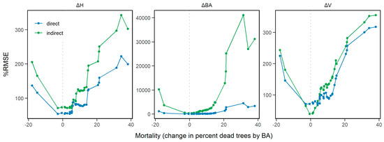
Figure 5.
Relationship between model accuracy (root mean square error (RMSE)%) and plot-level mortality defined as change in percent dead tree by basal area.
4. Discussion
This study had three main objectives. The first was to assess the predictive capability of ALS and DAP data for estimating plot-level growth in H, BA, and V; the second was to determine which approach (direct or indirect) is more suitable for estimating growth; and the last was to determine how the accuracy of growth predictions depend on the level of mortality. Predictive models were developed for H, BA, and V at T1 and T2 using ALS-based metrics for T1 models and DAP-based metrics for T2 models. Indirect estimates of growth were calculated as a difference between T1 and T2 model predictions, whereas separate models were developed to directly estimate the growth of H, BA, and V. Ground-plot measures indicated two confounding factors for growth assessment in this mixedwood boreal forest environment: Slow growth rates for H, BA, and V, as well as relatively high levels of mortality (Table 1).
We found that the direct approach resulted in more accurate estimates of growth for all three of the selected stand attributes. Results showed that the direct predictions of ∆H were by far the most accurate, while indirect models of ∆BA and ∆V were not suitable for predicting growth. When the change in forest attribute was calculated based on the difference between T1 and T2 models, estimation errors from the T1 and T2 models were compounded. This effect increased with the decrease of accuracy of the T1 and T2 models, which was especially pronounced for the indirectly derived ∆BA and ∆V. Though the accuracy of the individual models for BA and V at T1 and T2 was on par with accuracies reported in the literature for similar forest stand conditions [24,50], the analyses show that this level of accuracy was insufficient for determining growth in these stand conditions.
Our results are similar to those of Cao et al. [26] and Bollandsås et al. [51], who also found the direct approach to provide superior results when modeling forest growth. In their study, Cao et al. [26] used to two ALS datasets acquired over six year period to estimate forest biomass dynamics. The authors reported that the direct model had an R2 value of 0.63 and an RMSE% of 25.64%. Bollandsås et al. [51] used two ALS datasets to estimate change in above ground biomass. Authors found that the direct method gave best results, with an RMSE between 1.9 and 21.7 Mg ha−1. In our case, the lower accuracy of the growth predictions may have resulted from much slower tree growth—with a seven-to-nine year difference between ALS and DAP data acquisitions, the increase in tree size was very often lower than the error of the developed models. Given a mean H growth rate of 0.12 m yr−1 in this set of plots (Table 1), approximately 14 years (an additional, approximately, seven years) would be required for the growth to exceed the modeling error reported herein. Moreover, as a result of the lower accuracy of ∆VD, approximately 22 years would be required for the growth to exceed the error associated with the volume estimates.
We found that stand mortality affects the prediction accuracy of the change models and that the impact of mortality on model outcomes is similar for both the indirect and direct approach. The reference data used to calibrate the models did not include dead trees (i.e., plot-level summaries of H, BA, and V were calculated using living trees only); however, the presence of dead standing trees in a plot will contribute to the point cloud metrics and impact the developed models. ALS returns from snags in or above the canopy may have affected the point cloud metrics used in modeling by either obscuring live trees or by modifying the plot’s canopy surface.
This paper demonstrates a number of challenges related to assessing forest growth using bi-temporal point cloud datasets acquired with two different technologies. These challenges originate not only from the type of data used (ALS vs. DAP) but also from the time interval between data acquisitions, the growth rate of the forests, and the level of stand mortality. Our results showed that even for forest stand attributes like H, which is among the most accurately predicted with point cloud data, estimates of growth are not accurate (RMSE% exceeding 150% for the most accurate estimates of growth). Considering that the typical accuracy of stand attributes like BA or V is lower, estimating change in these attributes using the direct or indirect approach was even more challenging in the stand conditions present in this study. Though extending the time between the data acquisitions may result in more accurate predictions of stand growth, it may not be desirable from a forest management perspective if more frequent data are required to update for disturbances.
Alternative methods for estimating forest growth that may be used in highly disturbed, slow growing forest stands like the ones analyzed in this study involve linking the point cloud-based estimates of stand attributes to growth simulators. For example, Lamb et al. [23] demonstrated how ALS-predicted stand attributes can be matched with a library of plot-level measurements and used as inputs for a locally calibrate tree-list growth model. Forest stand attributes predicted with point cloud data can also be integrated with stand-level growth models by generating a database of growth curves and using cell-level predictions to identify the most suitable growth curve [24,52]. Though such approaches benefit from a bi-temporal dataset, they can be used with a single ALS acquisition. They are also less prone to errors originating from the time difference between data acquisitions (when two or more datasets are used) or growth rate—the growth is determined by the existing growth model, rather than calculated using the predictions derived from the data.
Despite recent technological advancements, ALS data collection currently remains a relatively expensive option for monitoring forest growth over large forest areas. However, ALS, in a forestry context, contributes to a full suite of applications including forest operations, inventory, planning, and management for a broad suite of ecosystem goods and services. ALS acquisitions are also necessary for the production of a high-quality and detailed DTM and high-quality attribute estimates, which, together, can largely balance the costs from the data’s collection and processing [53]. The province of Alberta, in which this study took place, has invested in near wall-to-wall acquisition of ALS data between 2003 and 2014 and is interested in maximizing the utility of the existing data set [54]. By supplementing ALS data acquisitions with DAP, the forest industry can save on operational costs [8] and provide other predictive statistics including spectral tone, texture, and pattern [55]. These metrics have been valuable in quantifying other forest attributes that are challenging to resolve using ALS, such as species composition and health status [56]. They also serve well for other forest applications including the monitoring of the mountain pine beetle [57], monitoring forest fires [58], or tree species identification [59]. However, the capacity of these data to support growth assessments in the highly disturbed and slow growing forests of the mixedwood boreal was not demonstrated in this study. What is clear from the results presented herein is that empirical estimates of growth derived from point cloud data in this forest environment require sufficient time between data acquisitions, rigorous ground plot measurements and plot-level estimates of mortality.
5. Conclusions
This study exemplifies the challenges of growth monitoring in a structurally complex mixedwood forest environment using a bi-temporal and multi-sensor approach. Focusing on three stand attributes including H, BA, and V, we demonstrated the accuracy of estimating growth in forest attributes using low density ALS and DAP point cloud datasets, direct and indirect modeling approaches, and the impact of mortality on the accuracy of growth estimates. We conclude that the accuracy of the stand attributes derived with ALS- and DAP-based predictors was similar. Estimates of growth were inaccurate for BA and V, and we recommend the direct approach when modeling ∆H. The accuracy of the predictive models decreased with increasing plot-level mortality, and minimizing plot-level mortality effectively maximized the accuracy of predictions. Regardless, the low accuracy of the optimized models demonstrates that a multi-sensor approach to growth monitoring using ALS and DAP is better suited to forest environments with lower mortality and/or faster growth rates.
Future studies in multi-sensor growth should concentrate on attribute estimation and modeling approach optimization. More research is required to assess the combination of ALS and DAP data to estimate forest growth in unmanaged boreal forests, particularly with respect to basal area and gross total volume.
Author Contributions
Conceptualization, P.T., J.R., N.C.C., J.C.W., A.N.V.G., and K.R.; methodology, P.T., J.R., A.N.V.G., N.C.C., and J.C.W.; software, P.T., J.R., A.N.V.G.; formal analysis, P.T., J.R.; investigation, P.T., J.R.; writing—original draft preparation, P.T., J.R.; writing—review and editing, N.C.C., J.C.W., A.N.V.G., K.R.
Funding
This research was funded by the AWARE (Assessment of Wood Attributes using Remote Sensing) Natural Sciences and Engineering Research Council of Canada Collaborative Research and Development grant to a team led by Nicholas Coops with support in this study from West Fraser.
Acknowledgments
We thank the staff at West Fraser, Alberta Agriculture and Forestry (Chris Bater, Barry White) for their input and assistance with the project.
Conflicts of Interest
The authors declare no conflict of interest. The funders had no role in the design of the study; in the collection, analyses, or interpretation of data; in the writing of the manuscript, or in the decision to publish the results.
References
- Canada’s National Forest Inventory. Available online: https://nfi.nfis.org/en/ (accessed on 1 July 2019).
- Meyer, V.; Saatchi, S.S.; Chave, J.; Dalling, J.W.; Bohlman, S.; Fricker, G.A.; Robinson, C.; Neumann, M.; Hubbell, S. Detecting tropical forest biomass dynamics from repeated airborne lidar measurements. Biogeosciences 2013, 10, 5421–5438. [Google Scholar] [CrossRef]
- Vanclay, J.K. Modelling Forest Growth and Yield: Applications to Mixed Tropical Forests; CAB International: Wallingford, UK, 1994; ISBN 0-85198-913-6. [Google Scholar]
- Woods, M.; Pitt, D.; Penner, M.; Lim, K.; Nesbitt, D.; Etheridge, D.; Treitz, P. Operational implementation of a LiDAR inventory in Boreal Ontario. For. Chron. 2011, 87, 512–528. [Google Scholar] [CrossRef]
- Fardusi, M.J.; Chianucci, F.; Barbati, A. Concept to practices of geospatial information tools to assist forest management & planning under precision forestry framework: A review. Ann. Silvic. Res. 2017, 41, 3–14. [Google Scholar] [CrossRef]
- White, J.C.; Wulder, M.A.; Varhola, A.; Vastaranta, M.; Coops, N.C.; Cook, B.D.; Pitt, D.; Woods, M. A best practices guide for generating forest inventory attributes from airborne laser scanning data using an area-based approach. For. Chron. 2013, 89, 722–723. [Google Scholar] [CrossRef]
- Van Leeuwen, M.; Nieuwenhuis, M. Retrieval of forest structural parameters using LiDAR remote sensing. Eur. J. For. Res. 2010, 129, 749–770. [Google Scholar] [CrossRef]
- White, J.C.; Wulder, M.A.; Vastaranta, M.; Coops, N.C.; Pitt, D.; Woods, M. The Utility of Image-Based Point Clouds for Forest Inventory: A Comparison with Airborne Laser Scanning. Forest 2013, 4, 518–536. [Google Scholar] [CrossRef]
- St-Onge, B.; Vega, C.; Fournier, R.A.; Hu, Y. Mapping canopy height using a combination of digital stereo-photogrammetry and lidar. Int. J. Remote Sens. 2008, 29, 3343–3364. [Google Scholar] [CrossRef]
- Zimble, D.A.; Evans, D.L.; Carlson, G.C.; Parker, R.C.; Grado, S.C.; Gerard, P.D. Characterizing vertical forest structure using small-footprint airborne LiDAR. Remote Sens. Environ. 2003, 87, 171–182. [Google Scholar] [CrossRef]
- Reutebuch, S.E.; McGaughey, R.J.; Andersen, H.-E.; Carson, W.W. Accuracy of a high-resolution lidar terrain model under a conifer forest canopy. Can. J. Remote Sens. 2003, 29, 527–535. [Google Scholar] [CrossRef]
- Jakubowski, M.K.; Guo, Q.; Kelly, M. Tradeoffs between lidar pulse density and forest measurement accuracy. Remote Sens. Environ. 2013, 130, 245–253. [Google Scholar] [CrossRef]
- Gauthier, S.; Bernier, P.; Kuuluvainen, T.; Shvidenko, A.; Schepaschenko, D. Boreal forest health and global change. Science 2015, 349, 819–822. [Google Scholar] [CrossRef]
- Gutsell, S.L.; Johnson, E.A. Accurately ageing trees and examining their height-growth rates: Implications for interpreting forest dynamics. J. Ecol. 2002, 90, 153–166. [Google Scholar] [CrossRef]
- Stadt, K.J.; Navratil, S.; Lieffers, V.J. Age structure and growth of understory white spruce under aspen. Can. J. For. Res. 1996, 26, 1002–1007. [Google Scholar]
- Gower, S.T.; Martin, J.L. Boreal mixedwood tree growth on contrasting soils and disturbance types. Can. J. For. Res. 2006, 36, 986–995. [Google Scholar]
- St-Onge, B. Estimating individual tree heights of the boreal forest using airborne laser altimetry and digital videography. Int. Arch. Photogramm. Remote Sens. 1999, 32, W14. [Google Scholar]
- St-Onge, B.; Vepakomma, U. Assessing forest gap dynamics and growth using multi-temporal laser-scanner data. Int. Arch. Photogramm. Remote Sens. Spat. Inf. Sci. 2004, 140, 173–178. [Google Scholar]
- Nasset, E.; Gobakken, T. Estimating forest growth using canopy metrics derived from airborne laser scanner data. Remote Sens. Environ. 2005, 96, 453–465. [Google Scholar] [CrossRef]
- Hopkinson, C.; Chasmer, L.; Hall, R. The uncertainty in conifer plantation growth prediction from multi-temporal lidar datasets. Remote Sens. Environ. 2008, 112, 1168–1180. [Google Scholar] [CrossRef]
- Yu, X.; Hyyppä, J.; Kaartinen, H.; Maltamo, M.; Hyyppä, H. Obtaining plotwise mean height and volume growth in boreal forests using multi-temporal laser surveys and various change detection techniques. Int. J. Remote Sens. 2008, 29, 1367–1386. [Google Scholar] [CrossRef]
- Vega, C.; Stonge, B. Height growth reconstruction of a boreal forest canopy over a period of 58 years using a combination of photogrammetric and lidar models. Remote Sens. Environ. 2008, 112, 1784–1794. [Google Scholar] [CrossRef]
- Lamb, S.M.; MacLean, D.A.; Hennigar, C.R.; Pitt, D.G. Forecasting Forest Inventory Using Imputed Tree Lists for LiDAR Grid Cells and a Tree-List Growth Model. Forest 2018, 9, 167. [Google Scholar] [CrossRef]
- Tompalski, P.; Coops, N.C.; Marshall, P.L.; White, J.C.; Wulder, M.A.; Bailey, T. Combining Multi-Date Airborne Laser Scanning and Digital Aerial Photogrammetric Data for Forest Growth and Yield Modelling. Remote Sens. 2018, 10, 347. [Google Scholar] [CrossRef]
- Stepper, C.; Straub, C.; Pretzsch, H. Using semi-global matching point clouds to estimate growing stock at the plot and stand levels: Application for a broadleaf-dominated forest in central Europe. Can. J. For. Res. 2015, 45, 111–123. [Google Scholar] [CrossRef]
- Cao, L.; Coops, N.C.; Innes, J.L.; Sheppard, S.R.; Fu, L.; Ruan, H.; She, G. Estimation of forest biomass dynamics in subtropical forests using multi-temporal airborne LiDAR data. Remote Sens. Environ. 2016, 178, 158–171. [Google Scholar] [CrossRef]
- Goodbody, T.R.H.; Coops, N.C.; Tompalski, P.; Crawford, P.; Day, K.J.K. Updating residual stem volume estimates using ALS- and UAV-acquired stereo-photogrammetric point clouds. Int. J. Remote Sens. 2016, 38, 2938–2953. [Google Scholar] [CrossRef]
- Coops, N.C.; Varhola, A.; Bater, C.W.; Teti, P.; Boon, S.; Goodwin, N.; Weiler, M. Assessing differences in tree and stand structure following beetle infestation using lidar data. Can. J. Remote Sens. 2009, 35, 497–508. [Google Scholar] [CrossRef]
- Kim, Y.; Yang, Z.; Cohen, W.B.; Pflugmacher, D.; Lauver, C.L.; Vankat, J.L. Distinguishing between live and dead standing tree biomass on the North Rim of Grand Canyon National Park, USA using small-footprint lidar data. Remote Sens. Environ. 2009, 113, 2499–2510. [Google Scholar] [CrossRef]
- Bright, B.C.; Hudak, A.T.; McGaughey, R.; Andersen, H.-E.; Negrón, J. Predicting live and dead tree basal area of bark beetle affected forests from discrete-return lidar. Can. J. Remote Sens. 2013, 39, S99–S111. [Google Scholar] [CrossRef]
- Natural Regions Committee. Natural Regions and Subregions of Alberta; Compiled by D.J. Downing and W.W. Pettapiece; Pub. No. T/852; Government of Alberta: Edmonton, AB, Canada, 2006; ISBN 0778545725.
- Huang, S.; Meng, S.X.; Yang, Y. A Growth and Yield Projection System (GYPSY) for Natural and Post-harvest Stands in Alberta. Tech. Rep. 2009, T/216, 1–22. [Google Scholar]
- Snavely, N.; Seitz, S.; Szeliski, R. Photo Tourism: Exploring Photo Collections in 3D. In ACM Transactions on Graphics; ACM: New York, NY, USA, 2006; pp. 835–846. [Google Scholar]
- Kamencay, P.; Breznan, M.; Jarina, R.; Lukac, P.; Zachariasova, M. Improved depth map estimation from stereo images based on hybrid method. Radioengineering 2012, 21, 79–85. [Google Scholar]
- Zhang, X.; Glennie, C.; Kusari, A. Change Detection From Differential Airborne LiDAR Using a Weighted Anisotropic Iterative Closest Point Algorithm. IEEE J. Sel. Top. Appl. Earth Obs. Remote Sens. 2015, 8, 1–9. [Google Scholar] [CrossRef]
- Gressin, A.; Mallet, C.; Demantké, J.Ô.; David, N. Towards 3D lidar point cloud registration improvement using optimal neighborhood knowledge. ISPRS J. Photogramm. Remote Sens. 2013, 79, 240–251. [Google Scholar] [CrossRef]
- Rusu, R.; Blodow, N.; Marton, Z.; Beetz, M. Aligning Point Cloud Views Using Persistent Feature Histograms. In Proceedings of the IEEE/RSJ International Conference on Intelligent Robots and Systems, Nice, France, 22–26 September 2008; pp. 3384–3391. [Google Scholar]
- Men, H.; Gebre, B.; Pochiraju, K. Color Point Cloud Registration with 4D ICP Algorithm. In Proceedings of the 2011 IEEE International Conference on Robotics and Automation, Shanghai, China, 9–13 May 2011; pp. 1511–1516. [Google Scholar]
- Nilsson, M. Estimation of tree heights and stand volume using an airborne lidar system. Remote Sens. Environ. 1996, 56, 1–7. [Google Scholar] [CrossRef]
- Roussel, J.R.; Auty, D. lidR: Airborne LiDAR Data Manipulation and Visualization for Forestry Applications; R package Version 2.1.1. Available online: https://github.com/Jean-Romain/lidR (accessed on 1 July 2019).
- R Core Team. R: A Language and Environment for Statistical Computing; R Foundation for Statistical Computing: Vienna, Austria, 2019. [Google Scholar]
- Bouvier, M.; Durrieu, S.; Fournier, R.A.; Renaud, J.-P. Generalizing predictive models of forest inventory attributes using an area-based approach with airborne LiDAR data. Remote Sens. Environ. 2015, 156, 322–334. [Google Scholar] [CrossRef]
- Robinson, A. Equivalence: Provides Tests and Graphics for Assessing Tests of Equivalence, R package version 0.7.2. 2016.
- Robinson, A.P.; Duursma, R.A.; Marshall, J.D. A regression-based equivalence test for model validation: Shifting the burden of proof. Tree Physiol. 2005, 25, 903–913. [Google Scholar] [CrossRef] [PubMed]
- Fekety, P.A.; Falkowski, M.J.; Hudak, A.T.; Jain, T.B.; Evans, J.S. Transferability of Lidar-derived Basal Area and Stem Density Models within a Northern Idaho Ecoregion. Can. J. Remote Sens. 2018, 44, 131–143. [Google Scholar] [CrossRef]
- Fekety, P.A.; Falkowski, M.J.; Hudak, A.T. Temporal transferability of LiDAR-based imputation of forest inventory attributes. Can. J. For. Res. 2015, 45, 422–435. [Google Scholar] [CrossRef]
- Penner, M.; Pitt, D.G.; Woods, M.E. Parametric vs. nonparametric LiDAR models for operational forest inventory in boreal Ontario. Can. J. Remote Sens. 2013, 39, 426–443. [Google Scholar] [CrossRef]
- McRoberts, R.E.; Bollandsås, O.M.; Næsset, E. Modeling and Estimating Change. In Forestry Applications of Airborne Laser Scanning Concepts and Case Studies; Springer: Dordrecht, The Netherlands, 2014; pp. 293–313. [Google Scholar]
- Hughes, I.G.; Hase, T.P.A. Measurements and their Uncertainties: A Practical Guide to Modern Error Analysis; Oxford University Press: New York, NY, USA, 2010; ISBN 978-0199566334. [Google Scholar]
- White, J.C.; Arnett, J.T.; Wulder, M.A.; Tompalski, P.; Coops, N.C. Evaluating the impact of leaf-on and leaf-off airborne laser scanning data on the estimation of forest inventory attributes with the area-based approach. Can. J. For. Res. 2015, 45, 1498–1513. [Google Scholar] [CrossRef]
- Bollandsås, O.M.; Gregoire, T.G.; Næsset, E.; Øyen, B.H. Detection of biomass change in a Norwegian mountain forest area using small footprint airborne laser scanner data. Stat. Methods Appl. 2013, 22, 113–129. [Google Scholar] [CrossRef]
- Tompalski, P.; Coops, N.C.; White, J.C.; Wulder, M.A. Enhancing Forest Growth and Yield Predictions with Airborne Laser Scanning Data: Increasing Spatial Detail and Optimizing Yield Curve Selection through Template Matching. Forest 2016, 7, 255. [Google Scholar] [CrossRef]
- White, J.C.; Tompalski, P.; Vastaranta, M.; Wulder, M.A.; Saarinen, S.; Stepper, C.; Coops, N.C. A Model Development and Application Guide for Generating an Enhanced Forest Inventory Using Airborne Laser Scanning Data and an Area-Based Approach; CWFC Information Report FI-X-018; Canadian Forest Service, Pacific Forestry Centre: Victoria, BC, Canada, 2017; 38p. [Google Scholar]
- Coops, N.C.; Tompalski, P.; Nijland, W.; Rickbeil, G.J.; Nielsen, S.E.; Bater, C.W.; Stadt, J.J. A forest structure habitat index based on airborne laser scanning data. Ecol. Indic. 2016, 67, 346–357. [Google Scholar] [CrossRef]
- Pitt, D.G.; Woods, M.; Penner, M. A Comparison of Point Clouds Derived from Stereo Imagery and Airborne Laser Scanning for the Area-Based Estimation of Forest Inventory Attributes in Boreal Ontario. Can. J. Remote Sens. 2014, 40, 214–232. [Google Scholar] [CrossRef]
- Wulder, M.; Bater, C.; Coops, N.C.; Hilker, T.; White, J.C. The role of LiDAR in sustainable forest management The role of LiDAR in sustainable forest management. For. Chron. 2008, 84, 807–826. [Google Scholar] [CrossRef]
- White, J.C.; Wulder, M.A.; Coggins, S.; Ortlepp, S.M.; Coops, N.; Heath, J.; Mora, B. Digital high spatial resolution aerial imagery to support forest health monitoring: The mountain pine beetle context. J. Appl. Remote Sens. 2012, 6, 062527. [Google Scholar] [CrossRef]
- Rufino, G.; Moccia, A. Integrated VIS-NIR Hyperspectral/Thermal-IR Electro-Optical Payload System for a Mini-UAV; Infotech Aerospace: Guerrero, Isabela, Puerto Rico, 2005. [Google Scholar]
- Gini, R.; Passoni, D.; Pinto, L.; Sona, G. Aerial images from an uav system: 3d modeling and tree species classification in a park area. ISPRS Int. Arch. Photogramm. Remote Sens. Spat. Inf. Sci. 2012, 39, 361–366. [Google Scholar] [CrossRef]


© 2019 by the authors. Licensee MDPI, Basel, Switzerland. This article is an open access article distributed under the terms and conditions of the Creative Commons Attribution (CC BY) license (http://creativecommons.org/licenses/by/4.0/).