Development of an Operational Algorithm for Automated Deforestation Mapping via the Bayesian Integration of Long-Term Optical and Microwave Satellite Data

Abstract

The frequent fine-scale monitoring of deforestation using satellite sensors is important for the sustainable management of forests. Traditional optical satellite sensors suffer from cloud interruption, particularly in tropical regions, and recent active microwave sensors (i.e., synthetic aperture radar) demonstrate the difficulty in data interpretation owing to their inherent sensor noise and complicated backscatter features of forests. Although the sensor integration of optical and microwave sensors is of compelling research interest, particularly in the conduct of deforestation monitoring, this topic has not been widely studied. In this paper, we introduce an operational algorithm for automated deforestation mapping using long-term optical and L-band SAR data, including a simple time-series analysis of Landsat stacks and a multilayered neural network with Advanced Spaceborne Thermal Emission and Reflection Radiometer and Phased Array-type L-band Synthetic Aperture Radar-2, followed by sensor integration based on the Bayesian Updating of Land-Cover. We applied the algorithm over a deciduous tropical forest in Cambodia in 2003–2018 for validation, and the algorithm demonstrated better accuracy than existing approaches, which only depend on optical data or SAR data. Owing to the cloud penetration ability of SAR, observation gaps of optical data under cloudy conditions were filled, resulting in a prompter detection of deforestation even in the tropical rainy season. We also investigated the effect of posterior probability constraints in the Bayesian approach. The land-cover maps (forest/deforestation) created by the well-tuned Bayesian approach achieved 94.0% ± 4.5%, 80.0% ± 10.1%, and 96.4% ± 1.9% for the user’s accuracy, producer’s accuracy, and overall accuracy, respectively. In the future, small-scale commission errors in the resultant maps should be improved by using more sophisticated machine-learning approaches and considering the reforestation effects in the algorithm. The application of the algorithm to other landscapes with other sensor combinations is also desirable.

1. Introduction

Forests play important roles in the maintenance of the ecosystem, watershed control, and carbon and/or water cycle. The irreversible loss of forests (i.e., deforestation) leads to greenhouse gas emission that cause climate change [1], wildlife habitat loss [2], and vulnerable ground conditions that may cause sediment disasters [3]. According to the Global Forest Resources Assessment, global forested areas decreased by 129 million ha from 1999 to 2015 [4]. The areas experiencing the most severe deforestation are in tropical regions, including South America [5], Africa [6], and Southeast Asia [7]. This issue has led to several international conventions for forest conservation, such as Reducing Emissions from Deforestation and forest Degradation (i.e., REDD+) [8]. In such frameworks, the importance of continuous and near-real-time monitoring of forests has been repeatedly indicated.

Satellite remote sensing is an essential tool for continuous monitoring, particularly in tropical regions, where in-situ surveys are laborious and expensive. Researchers have developed monitoring methods by using moderate-resolution optical sensors [9,10,11,12] and microwave sensors [13,14,15], resulting in the development of several automated mapping systems for deforestation, such as Global Land Analysis and Discovery (GLAD) alerts [16] and JJ-FAST, the early-warning system in the tropics provided by Japan Aerospace Exploration Agency (JAXA) and Japan International Cooperation Agency (JICA) [17]. Optical sensor data are relatively easy to interpret and obtain using various open-free archives, such as the Landsat series, which is used in GLAD, and Moderate-Resolution Imaging Spectroradiometer (MODIS). However, the most problematic issue attached to these sensors is their inability to perform ground observations under cloudy or hazy conditions. This is particularly problematic in tropical regions, where cloud frequently covers the ground [18,19]. By contrast, active microwave sensors (i.e., synthetic aperture radars), which are used in JJ-FAST, can provide fine-resolution maps, regardless of the cloud conditions, with their built-in ability to penetrate through clouds. The microwave backscatter from the forest is sensitive to the biomass of the forest [20], particularly in the horizontal–vertical (HV) polarization. Therefore, it is useful to separate forest and deforested areas. Nonetheless, microwave sensors face issues, such as the interpretation difficulty caused by inherent sensor noise (i.e., speckle noise), the complicated features of the microwave backscatter, and the limited access to open-free data (Sentinel-1 is only available for long-term SAR archives so far).

Given such contrasting features, the integrated use of optical and microwave sensors has been an attractive research interest for cloud-free and accurate deforestation monitoring. Research on sensor fusion has traditionally focused mainly on optical–optical fusion (i.e., fusion between two optical sensors of different resolutions) using a reconstruction-based approach (e.g., [21,22]) and not on optical–microwave fusion [23]. The largely different observation mechanisms of optical and microwave sensors disallow application of the reconstruction-based approach, which assumes a physical similarity of the sensors to be fused. This problem motivated us to use a machine-learning-based approach instead. Mizuochi et al. The studies in [24,25] provided machine-learning- or statistic-based approaches for optical–microwave and passive microwave–active microwave fusions for seasonal wetland monitoring. Although such approaches seem promising for deforestation monitoring, the approaches of Mizuochi et al. [24,25] assume the seasonality of pixel change and use passive microwave data with coarse resolution (approximately 10 km) as their main inputs. Given that deforestation occurs in a smaller scale (around several tens of meters), the utilization of passive microwave sensors may not seem suitable. Moreover, another difference of deforestation events from the inundation of seasonal wetlands is their spatial randomness and one-time-only nature, i.e., historical deforestation training data for the same pixel are not repeatedly available. Therefore, an approach that depends on past match-ups is not suited for deforestation surveillance.

Reiche et al. [14] suggested the practicality of deforestation monitoring with an optical–SAR integration based on a statistical approach. They utilized Landsat, Sentinel-1, and the Phased Array type L-band Synthetic Aperture Radar-2 (PALSAR-2) to monitor deforestation with a mean time lag of 22 days. However, the proposed algorithm was only validated in one tropical dry forest (Bolivia) and was dependent on the window size for normalization treatment in image processing. The exploration of another operational method and evaluation in another landscape could add value to deforestation monitoring and contribute to forest conservation frameworks.

Here, (1) two different deforestation mapping approaches (a time-series analysis and a multilayered neural network) corresponding to each sensor’s feature and (2) the flexible integration of the derived maps from different sensors via Bayesian Updating of Land-Cover (BULC) are provided. The applicability of BULC, which was originally proposed by Cardille and Fortin [26] for a consistent time-series update of the land-cover map, is investigated in the current study for its extension in a sensor fusion context. We tried to make the algorithm satisfy the following:

(1)

Scalable. It can flexibly integrate with any available data, regardless of the region of interest.

(2)

Best effort. An operation can proceed even when with some input data missing.

(3)

Robust. It is not very sensitive to sensor noise, cloud/cloud-shadow contamination, or seasonal deciduous forest changes.

(4)

Near-real-time: It can provide a deforestation map soon after obtaining a new satellite image. Alternatively, a computationally expensive algorithm or an algorithm that requires the overall recalculation of historical images is undesirable.

(5)

Accessible: It substantially utilizes open–free or cost-effective data, or its program is written via open-source software (e.g., Python, Bash, GRASS GIS).

The objectives of this research are to develop an operational algorithm for deforestation mapping and show a practical example of the BULC application. The focus of this research is limited to the early and one-time detection of deforestation, but we did not evaluate reforestation. Forest degradation (subpixel-scale forest thinning) is also out of our scope. To meet the requirements of accessibility and robustness, we chose long-term, open-free optical data (Landsat, Advanced Spaceborne Thermal Emission, and Reflection Radiometer (ASTER)) and long-term microwave data (i.e., PALSAR-2). We did not use Sentinel-1 even though the data are freely available, owing to the shorter penetration depth of C-band microwaves through the forest canopy [27], resulting in a poorer ability to separate forest/deforestation (as confirmed in a preliminary test over the study site). PALSAR-2 is not open-free, but JAXA freely provides data under frequent research announcements on earth observations.

2. Materials and Methods

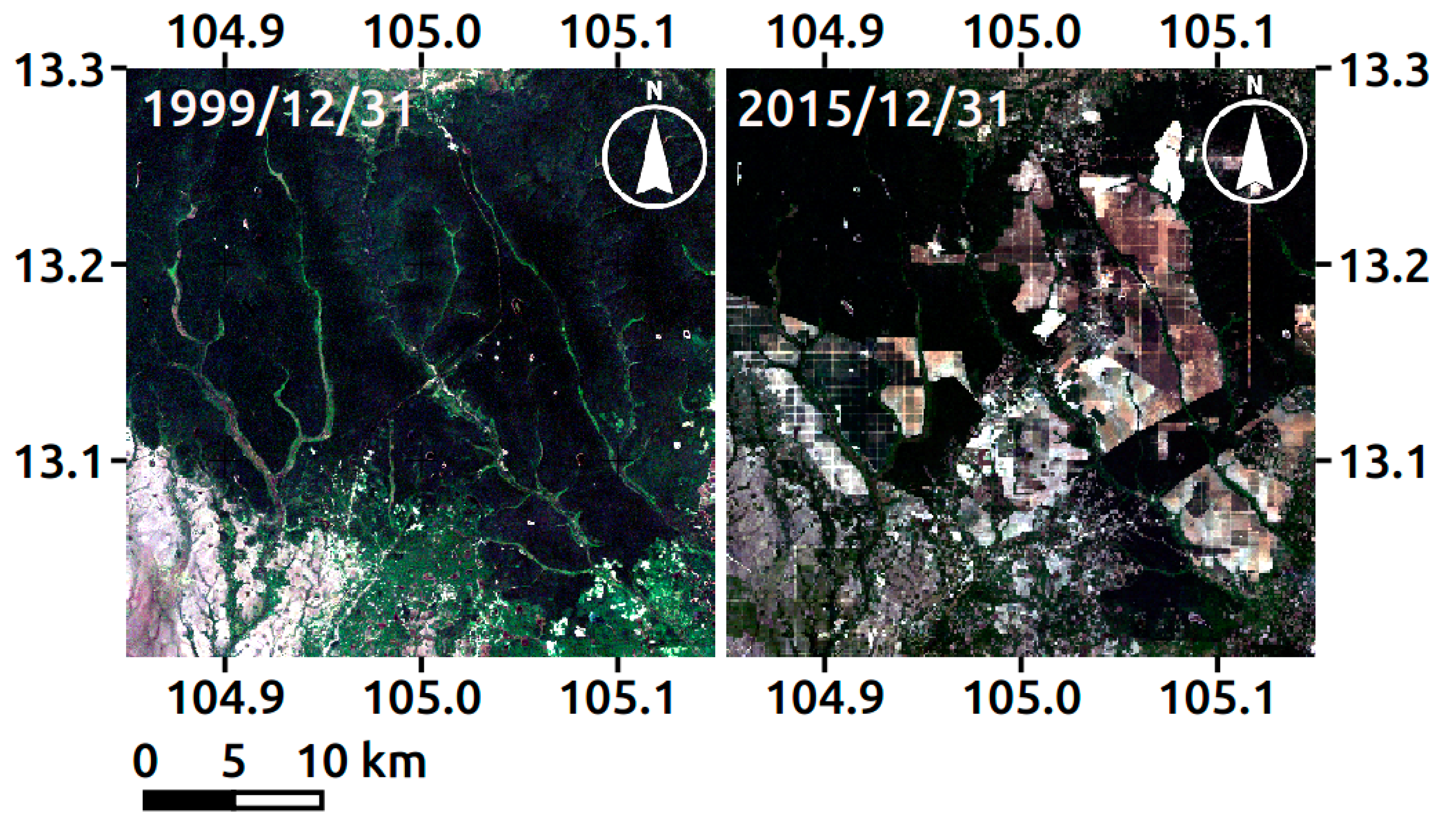
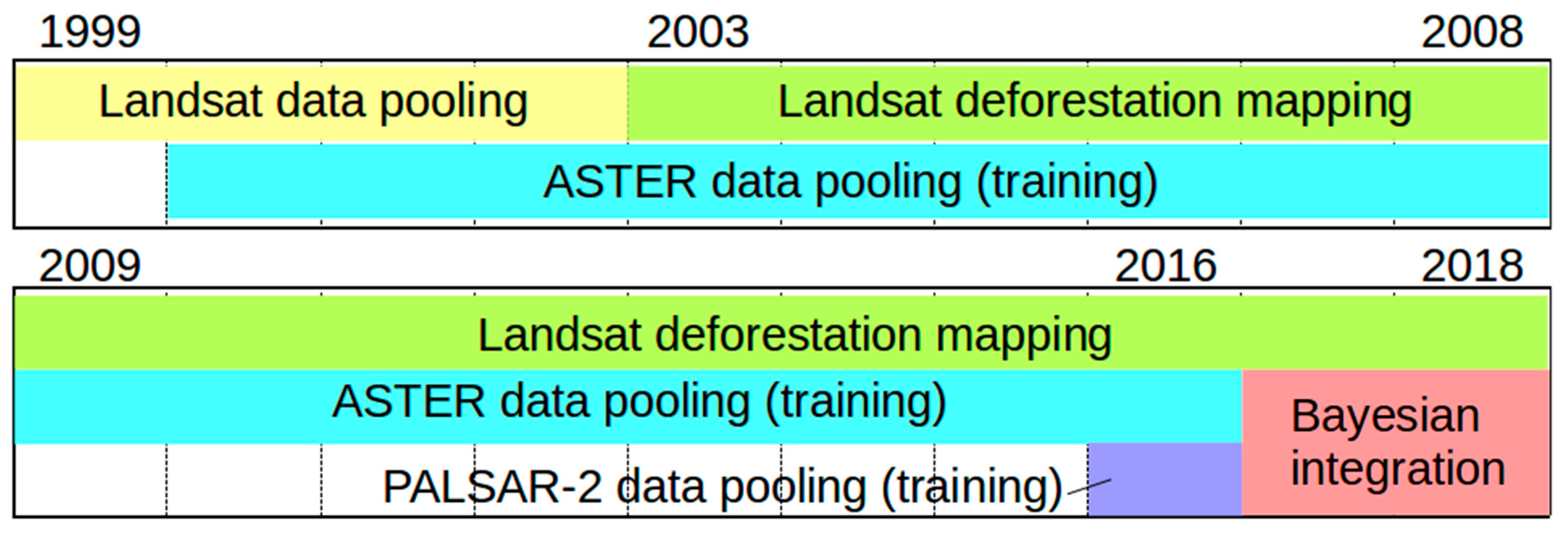
2.1. Study Site and Target Period

The study site was a forest in Cambodia (105.20E–105.50E, 12.80N–13.10N). Although the original land cover of the site is a deciduous forest, this site has been characterized by frequent and large-scale deforestation during the last decade (Figure 1), thus making it a suitable area for algorithm development and evaluation.

The study period was from 1999 to 2018, during which Landsat Thematic Mapper (TM), Enhanced Thematic Mapper Plus (ETM+), and Operational Land Imager (OLI) data were continuously usable. ASTER and PALSAR-2 data have been available since 2000 and 2016, respectively. Given the overlapping duration of each sensor and algorithm procedure (see Section 2.4), we defined (1) the data pooling (or training) period, (2) the Landsat-only deforestation mapping period, and (3) the sensor integration period (Figure 2). The data taken during the pooling period were only used to initialize the statistical parameters in the time-series analysis (see Section 2.4.1) or to train the neural network (see Section 2.4.2) and were not directly used for mapping. From 2003 to 2016, Landsat was the only sensor to map deforestation because the available ASTER and PALSAR-2 data were only used to the train the algorithm. During 2017–2018, ASTER and PALSAR-2 were also used for deforestation mapping, in addition to Landsat, and all the sensor data were integrated by BULC. To compare the BULC results with the single-sensor results, we also continued performing Landsat-only deforestation mapping (even during 2017–2018) separately from the BULC processing.

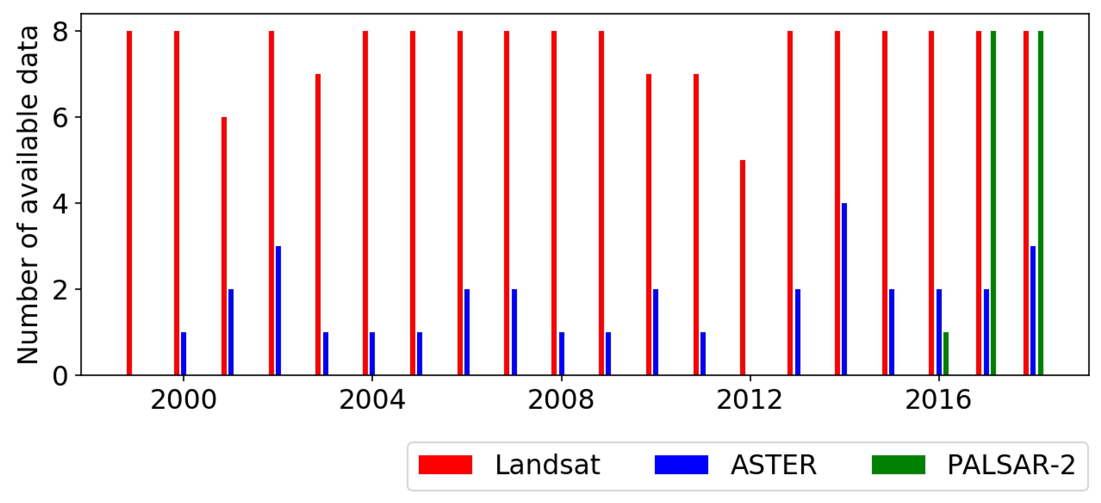
2.2. Satellite Data and Preprocessing

2.2.1. Landsat Series

Landsat is one of the most popular freely available satellite data series. Orthorectified surface reflectance images in visible to short-wave infrared (i.e., optical) bands with moderate spatial resolution (30 m) were provided by the US Geological Survey. For the study period, all available Landsat 5 (TM), 7 (ETM+), and 8 (OLI) data over the study site were downloaded via Google Earth Engine (GEE) [28]. In GEE, each pixel was preliminary cloud/cloud-shadow screened by referring to the quality assurance (QA) data provided together. The images were then temporally composited with a 1.5-month interval by taking the median of all images obtained within the period for each pixel. This treatment also helps screen out outlying pixels with cloud/cloud-shadow contamination or sensor errors. On the basis of previous reports, we assumed that all Landsat series data were interchangeable (e.g., [29,30]).

Even after the preliminary QA check and the median composite, we still found nonnegligible thin-cloud and cloud shadows on the images. We ensured their elimination by additionally creating high-quality cloud/cloud-shadow masks using machine learning (support vector machine (SVM)). We collected reference data (labeled as cloud, cloud shadow, or clear) by pixel-based visual interpretation in typical cloudy Landsat scenes over the study site. We used the reference data to train SVM and to create a high-quality cloud/cloud-shadow mask. Furthermore, we created nonforest and water masks. The nonforest mask was created by visual interpretation of the Landsat images taken from 1999 to 2002, distinguishing the urban from the barren areas (i.e., areas where no trees had existed prior to the onset of the study period) from the forested area. The water mask, which includes rivers and a seasonally flooded area, was created for each scene on the basis of the modified normalized difference water index (MNDWI) value with a threshold value of 0.3, which was determined during the preliminary tuning.

We extracted deforestation signals from the quality-controlled Landsat data. Raster calculation was conducted to obtain the normalized difference vegetation index (NDVI) [31], MNDWI [32], and normalized difference soil index (NDSI) [33], which are defined as follows:

NDVI = (NIR − R)/(NIR + R)

(1)

MNDWI = (G − SWIR)/(G + SWIR)

(2)

NDSI = (SWIR − NIR)/(SWIR + NIR)

(3)

where R, G, B, NIR, and SWIR are the surface reflectance of red, green, blue, near-infrared, and short-wave infrared bands, respectively. Each index is sensitive to vegetation, surface wetness, and soil. In the deforestation pixel, we confirmed a decrease in NDVI and MNDWI, whereas NDSI increased significantly beyond the range of seasonal change, and this change corresponds to the land cover change from the vegetated area to the barren one. We also utilized hue information from the hue, saturation and value (HSV) transformation [34] from the original true color (red, green, and blue) images. With the color of the deforestation pixel changing from green (hue = 120°) to red (hue = 0°), the cosine and sine of the hue increased and decreased from these values, respectively.

2.2.2. ASTER

ASTER is an optical satellite sensor with a higher spatial resolution (15 m) than Landsat. Although it has a lower observation frequency than Landsat, ASTER can complement Landsat because of the former’s long operation duration. Orthorectified optical band images were provided by the National Institute of Advanced Industrial Science and Technology [35]. The original digital numbers (DN) were radiometrically and atmospherically corrected using 6S radiative transfer code and were transformed into surface reflectance. We created cloud/cloud-shadow and water masks by using the same procedure as that of Landsat. For simplicity of the analysis, we converted the original acquisition dates of ASTER to the nearest Landsat time step (i.e., a 1.5-month composite).

Moreover, unlike in Landsat, we applied a multilayered neural network to ASTER for mapping deforestation (a detailed description of this procedure is provided in Section 2.4). To increase the dimension of feature vectors, we included texture information in addition to the original bands and spectral indices. We used the original red, green, and NIR bands, HSV from the false-color images, three calculable spectral indices (NDVI, normalized difference water index (NDWI), and green-red ratio vegetation index (GRVI)), and four textures (entropy, correlation, angular second moment, and contrast) of NDVI. NDWI [36] and GRVI [37] are defined as follows:

NDWI = (G − NIR)/(G + NIR)

(4)

GRVI = (G − R)/(G + R)

(5)

We did not calculate MNDWI (Equation (2)) and NDSI (Equation (3)) for ASTER because ASTER was not equipped with a blue band and was not SWIR-data accessible after 2008. A total of 14 feature images were created for each observation day and were used as input data for the neural network.

2.2.3. PALSAR-2

PALSAR-2 is an L-band synthetic aperture radar managed by JAXA. Orthorectified HH and HV polarization data in the broad-scale observation mode (ScanSAR) for 2016 to 2018 with an approximately 1.5-month observation frequency and 50 m spatial resolution were provided by JAXA. The original DN (intensity) was converted into a backscatter coefficient (γ⁰) by using the following:

γ⁰ = 10 log <DN²> + CF

(6)

where the bracket indicates the spatial average to mitigate speckle noise (a 3 × 3 moving window was applied for this case), and CF is a calibration factor constant of −83.0 [38]. Similar to ASTER, we converted the original acquisition date into the time step of Landsat. Thus, given such an occurrence, we averaged multiple PALSAR-2 data obtained within the 1.5-month duration.

Pseudo RGB composite images using the backscatter intensity of HH, HV, and HH/HV are often used for forest visualization [39]. To use this pseudo color information, we applied HSV transformation from the pseudo RGB. Furthermore, similar to the case of ASTER, we tried using the four-texture information of γ⁰ for the HV polarization. Texture values are sensitive to the forest biomass [40] and seem to be useful for establishing a distinction between forest and deforestation areas. A total of 10 feature images were created for each observation day and were used as input data for the neural network.

Moreover, image coregistration is important in sensor fusion. Thus, we visually checked for location errors for all images and found a nonnegligible location difference between the images of PALSAR-2 and those of other sensors. We fixed this location error by precisely applying the phase-only correlation method [41] and coregistered images.

Table 1. Sensor characteristics. Section 2.2 describes the details of the calculated features.

	Landsat	ASTER	PALSAR-2
Duration	1999–2018	2000–2018	2016–2018
Original resolution	30 m	15 m	50 m
Band used	optical	Optical	microwave
Calculated features	NDVI, MNDWI, NDSI, sin(hue), cos(hue)	red, green, blue, sin(hue), cos(hue), saturation, value, NDVI, NDWI, GRVI, NDVI-Entropy, NDVI-Correlation, NDVI-ASM, NDVI-Contrast	γ0HH, γ0HV, sin(hue), cos(hue), saturation, value, γ0HV-Entropy, γ0HV-Correlation, γ0HV-ASM, γ0HV-Contrast

summarizes all sensor characteristics and preprocessing, and Figure 3 illustrates the annual data availability for 1.5-month intervals (i.e., the largest amount corresponds to eight data points per year). Landsat was a main data source throughout the entire period while ASTER and PALSAR-2 provided complementary information to fill the gaps of Landsat.

2.3. Reference Data

In general, frequent in-situ reference data for deforestation are difficult to obtain. Therefore, for the purpose of training and validation, researchers often use visual interpretation of the long-term satellite data themselves [14]. On the contrary, reference (or validation) data should have higher quality than the data to be validated [42]. Therefore, we used Sentinel-2 images via GEE and high-resolution images of Google Earth, in addition to Landsat, ASTER, and PALSAR-2 images, for visual interpretation. Every 1.5-month interval for a 20-year period, we displayed available composite color images (true, false, or pseudocolor images depending on the used data) and looked for deforestation areas in the GIS software (QGIS 2.18), constructing deforestation polygons on the images. Past deforestation polygons were overlaid on the composite color images to reveal new deforestation areas. The created polygons were rasterized with the same spatial resolution as Sentinel-2 (10 m), and deduplicated between different time steps. The deduplication process ensured that only new deforestation areas were delineated in the reference map for each time step. Therefore, they are comparable to change-detection deforestation maps. The reference maps were used for the training of the neural network (Section 2.4) and for spatiotemporal validation.

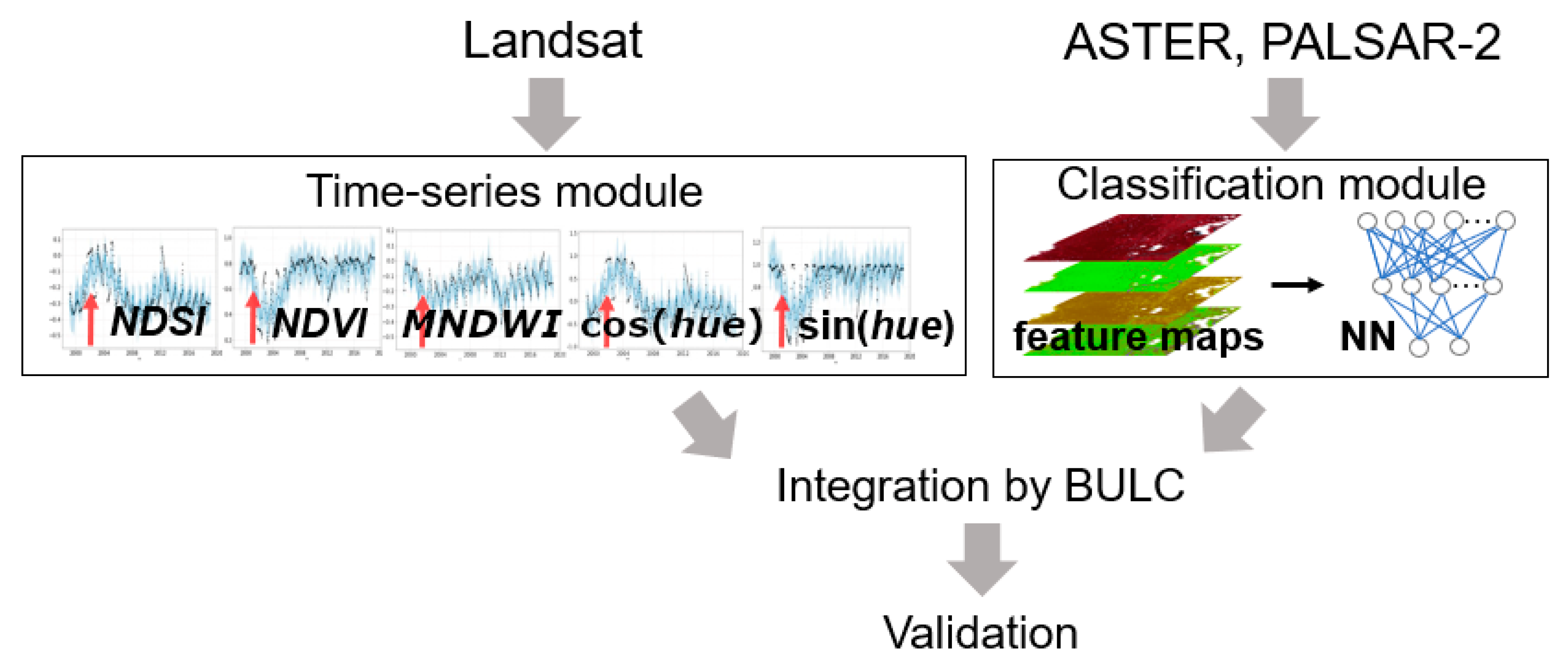
2.4. Algorithm

Figure 4 shows the overall flowchart of the algorithm. We first created deforestation maps from each sensor. Considering the data availability, we selected different approaches for Landsat (i.e., time-series analysis) and ASTER/PALSAR-2 (i.e., classification by the neural network). We resampled the constructed deforestation maps into the same spatial resolution of reference as that for Sentinel-2 (10 m) and then integrated the time-series deforestation maps by BULC. Finally, we validated the integrated map using the reference and compared the accuracy to that of other existing deforestation maps, such as those created by Hansen et al. [12] and JAXA [17].

2.4.1. Time-series module

We could apply a simple time-series analysis for the large and dense data archive provided by Landsat to detect changes. By making use of the significant and irreversible change of the five indices (NDVI, MNDWI, NDSI, cosine, and sine of hue), we applied the procedure described in the following. For an index f at pixel (i, j) on day t,

• Calculate the mean μ_f and standard deviation σ_f of f during day 1, 2, …, t − 1.
• Flag the pixel where f(t, i, j) satisfies the following:
  f (t, i, j) < μ_f–2 σ_f (f: NDVI, MNDWI, sin(hue)), or
  f (t, i, j) > μ_f + 2 σ_f (f: NDSI, cos(hue)).
• Determine the pixel as deforestation if more than four indices are flagged.

To appropriately consider the seasonal change and sensor noise as a “natural” statistical fluctuation, we pooled four-year data and started the procedure from 2003.

2.4.2. Classification Module

Since ASTER and PALSAR-2 provide a limited amount of data compared to Landsat, we could not implement a time-series analysis, which requires a sufficient number of data. Instead, we decided to use image classification via a multilayered NN consisting of a 14-node or 10-node input layer with an 8-node first hidden layer followed by a 2-node second hidden layer and an output layer, which judges forest or deforestation by using the softmax function. The softmax function, also known as the normalized exponential, is a multiclass generalization of the logistic sigmoid [43] and is often used as an activation function of the NN output layer. The other parameters (shown in

Table 2. Parameter setting for the multilayered neural network.

Activation function	ReLu
Cost function	Cross entropy
Regularization rate (L1 regularization)	0.0005
Dropout rate	0.15
Minibatch size	512

) were tuned on the basis of the preliminary test. The NN was trained by the reference data during the data pooling period (i.e., 2000–2016 for ASTER and 2016 for PALSAR-2) and was used to map deforestation for 2017–2018. For each sensor, we sampled a total of 10 million pixels, which were used as the training data.

2.4.3. Postintegration of Multiple Deforestation Maps

We integrated the deforestation maps created from each sensor by BULC, which utilized an extended Bayes’ theorem. Theoretically, the integration enabled the reconstruction of a consistent land-cover transition from multiple land-cover data sources, which originally contained errors and inconsistency between sensors and between observations. When a new observation E of a land cover c2 was obtained in a day (or order) i + 1, the posterior probability of the true class L of land cover c1 was expressed as follows:

$$P\left(L_{c1,i+1}|E_{c2,i+1}\right)=\frac{P\left(E_{c2,i+1}|E_{c1,i}\right)\ast P\left(L_{c1,i}\right)}{{{\displaystyle \sum }}_{k=1,\dots ,n}P\left(E_{c2,i+1}|E_{ck,i}\right)\ast P\left(L_{ck,i}\right)}$$

(7)

where n is the number of total classes (in this case, n = 2; i.e., forest or deforestation). P(E_{c2, i+1}|E_c1,i) is the likelihood estimated by the following:

$$P\left(E_{c2,i+1}|E_{c1,i}\right)=\frac{P\left(E_{c2,i+1}\cap E_{c1,i}\right)}{P\left(E_{c1,i}\right)}$$

(8)

where P(L_c1,i) is the prior probability and can be replaced by the posterior probability in the previous time step i − 1. For i = 0, we assumed the prior (initial) probability by using the forest/nonforest map of the first day, as exemplified by Cardille and Fortin [26]. Specifically, we assign the initial probability of 0.6 and 0.4 for the forest and deforestation, respectively, should the pixel be classified as a forest in the nonforest mask that we created from the visual interpretation (Section 2.2), and vice versa. Moreover, Equation (8) can be calculated by comparing the land-cover maps on day i and day i + 1 to create a confusion matrix as if the day i map were the reference map, and the likelihood were the producer’s accuracy (PA). After the calculation of the posterior probability for both classes (forest and deforestation), we classified the class as a class with a higher posterior probability. Although the sensor integration period was in 2017–2018, we started running BULC from 2003 to stably estimate the prior probability for each time step before the integration period.

In the practical use of the Bayesian approach, we need to be careful that the likelihood and prior probability of a class are not zero. These are well-known issues called the zero frequency problem [44] and zero priors paradox [45]. The former can be mitigated by Laplace smoothing [44], i.e., by adding one to all the cells in the confusion matrix. The latter is often treated by replacing zero with a small but nonzero value (known as Cromwell’s rule [46]), although there is no consensus on which value should be replaced. Fortin et al. (2019) have also pointed out that BULC can get stuck when encountering zero probability [47]. Since we only had two classes for this study, there was a need to simultaneously replace the other class value (i.e., one) with a slightly smaller value when replacing zero with a slightly larger value for a class. Practically, the posterior probability (that will be used as prior probability at the next time step) must not vary in the full range [0,1] but in a narrower range. To investigate the effect of this constraint of the posterior probability, we attempted three scenarios and compared the results: (1) no constraint (i.e., accept zero), (2) a constraint within 0.05–0.95 (i.e., replace zero by 0.05 and one by 0.95), and (3) a constraint within 0.4–0.6.

Note that BULC does not integrate the change-detection maps but the land cover maps. In our case, the deforestation maps derived from ASTER and PALSAR-2 were land-cover maps, while those from Landsat were change-detection maps. Therefore, we accumulated the Landsat maps, beginning from the first day to the day of interest. The accumulated maps were assumed to be equivalent to the land-cover maps of forest/deforestation and were positioned together with the maps derived from ASTER and PALSAR-2 in the integration stage. In this sense, once a deforestation event was detected by Landsat, the pixel was assumed to be a permanent deforestation class in the succeeding period. This assumption corresponded to our research scope, where the focus was not on reforestation.

Lastly, we dealt with the order of sensor integration. During the Landsat-only period, we only needed to use BULC in a chronological order. However, during the sensor integration period, data from multiple sensors were often obtained at the same time step (i.e., 1.5-month interval). The last data became the most important because it determined the “conclusion” at the time step. We adopted these rules for setting the priority:

• Cloud-free data should come last.
• High-resolution data should come last.

For example, if the cloud fractional coverage values over the scenes were 80% and 40% for ASTER and Landsat, respectively, the integration order was ASTER, Landsat, and PALSAR-2. If all data were cloud free, the integration order was PALSAR-2, Landsat, and ASTER. The purpose of these rules is to avoid putting uncertain data in the last position. A cloudy image may cause classification errors due to the cloud or its shadow that remains even after quality control. Low-resolution images are also likely to lead to uncertain classification by missing subpixel-scale deforestation.

2.5. Validation and Evaluation

We converted the deforestation maps (land-cover maps) created by BULC into change-detection maps by subtraction during the period of interest. Subsequently, stratified random sampling [42,48] from the reference map was applied using the created map itself as a base map. This validation was performed both for the sensor integration period (2017–2018) and for the Landsat-only period (2003–2016). The sample size for both classes (i.e., forest and deforestation) was chosen as one twenty-fifth of the total amount of pixels of the class with the smallest area (forest or deforestation) in the base map, for each time step. This is because the coarsest source data in the analysis was PALSAR-2, whose spatial resolution (50 m) was five times that of the validation resolution (10 m). If we sampled over this threshold, multiple samples were likely to be taken from a narrow area (i.e., within one PALSAR-2 pixel), which were not independent of each other. The overall accuracy (OA), user’s accuracy (UA), PA, and their uncertainties, were estimated based on the guideline of Olofsson et al. (2014) [42]. To compare the accuracies with the products of Hansen et al. [12] and JAXA [17], we aggregated the original maps into a yearly time interval, which is the interval of Hansen et al. [12]. Furthermore, we created Landsat-only deforestation maps for 2017–2018. By comparing these maps with the BULC result, we were able to determine the effect of the sensor integration.

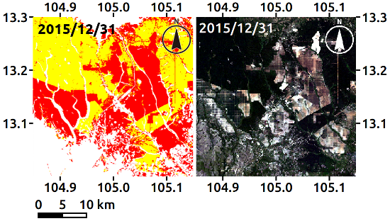
3. Results

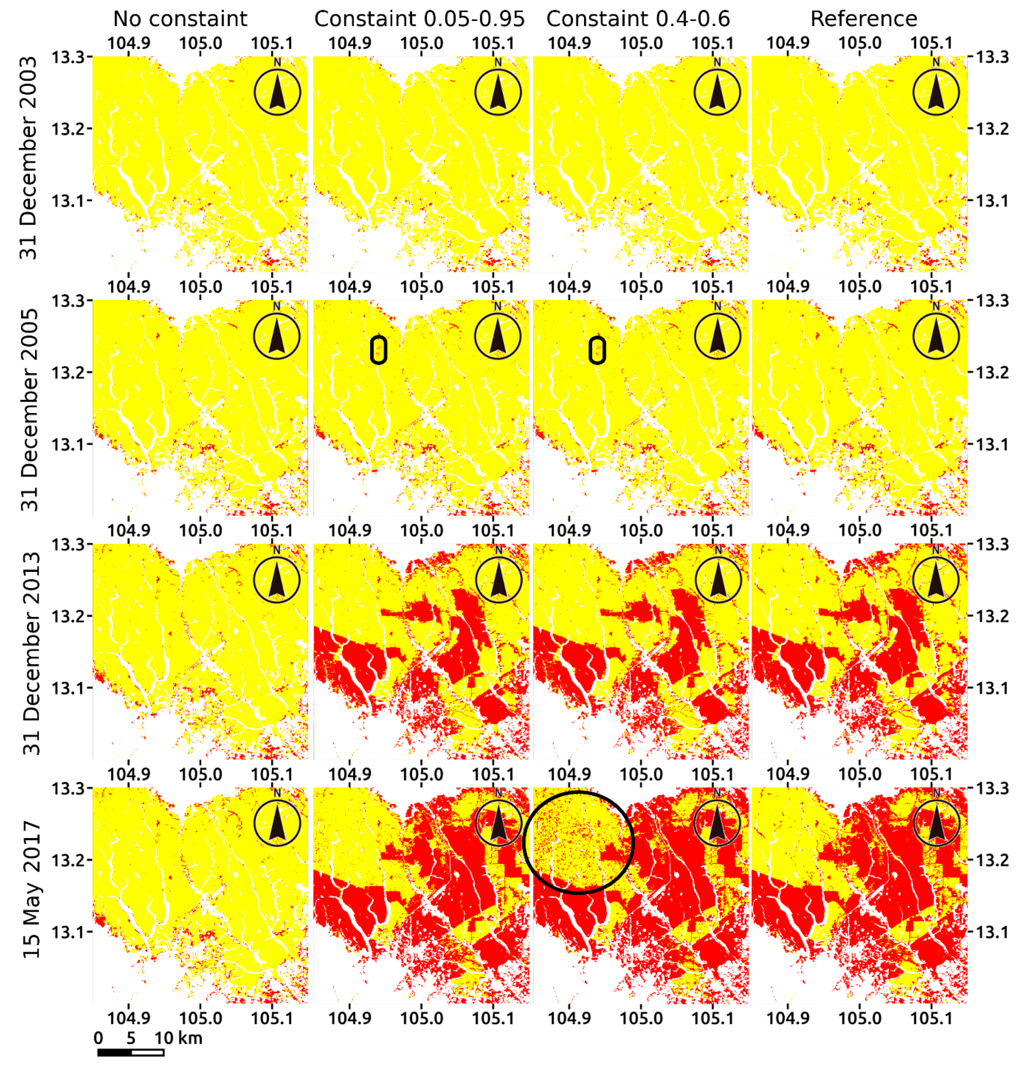
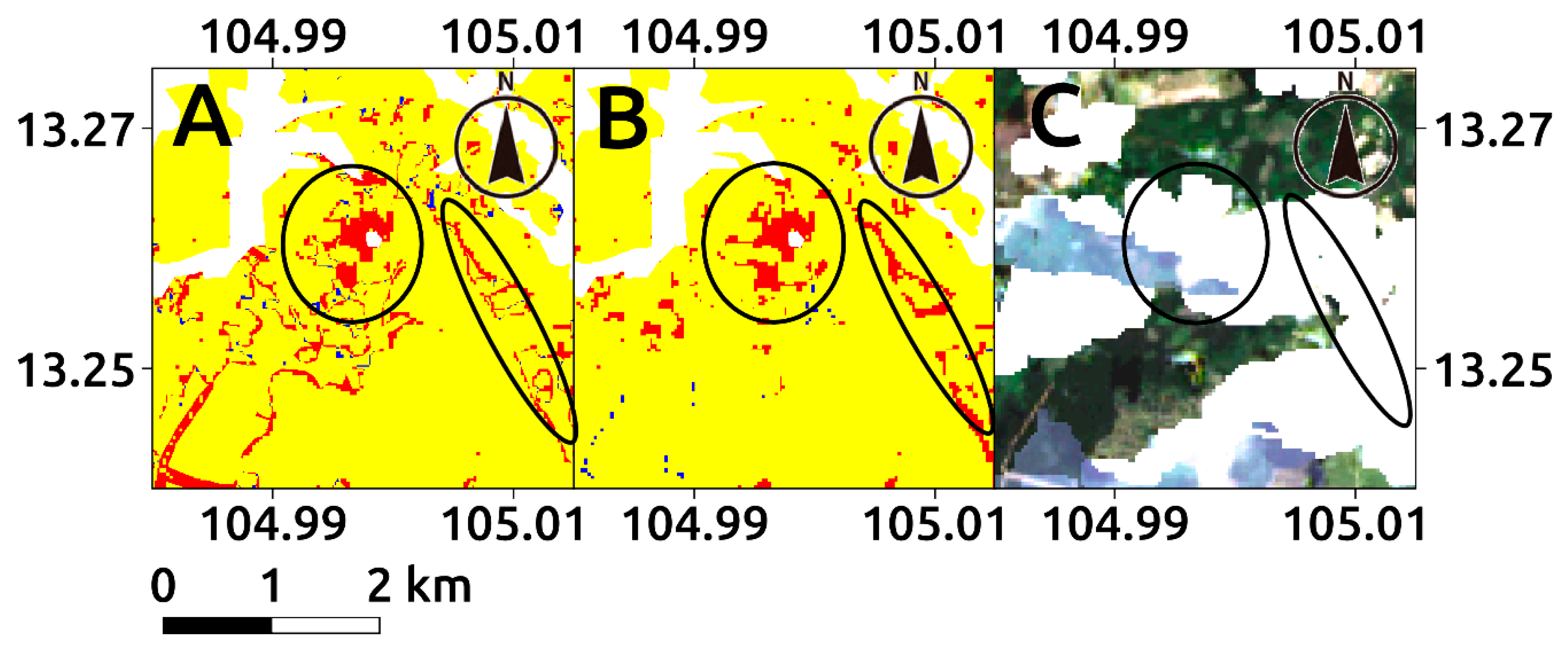
3.1. Effect of the Constraint of Posterior Probability

Figure 5 shows the deforestation maps created by BULC with different constraints for the posterior probability. Each map demonstrated a similar initial result regardless of the constraint. After a while (31 December 2005), a difference between the constraint and no-constraint maps appeared. We observed the error detections of deforestation in several areas of the constraint maps (e.g., the circled area in black). On the contrary, the no-constraint map initially showed robustness against noise. However, with the passing of time (31 December 2013), it displayed an apparent omission of deforestation. This “conservatism shift” of BULC was the very issue of the zero priors paradox; i.e., if we did not apply any constraint of the posterior probability, an area that has been a forest for a long time was likely to assume a forest classification forever, even with the occurrence of a new suspicious event, such as deforestation. The other two constraint maps did not show noticeable differences until the end of Landsat-only period but almost identically followed the original Landsat deforestation maps created by time-series analysis. However, in the sensor integration period (31 March, 2017), the constraint with a range of 0.4–0.6 showed less robustness against the errors of the other input data (mainly PALSAR-2). Consequently, the constraint with the 0.05–0.95 range showed the most consistent spatial pattern compared to the ground reference. Therefore, we adopted this constraint (0.05–0.95) for the next analysis. Moreover, in the land-cover maps (not the change-detection maps) for deforestation with the constraint, the averaged UA, PA, and OA were 94.0% ± 4.5%, 80.0% ± 10.1%, and 96.4% ± 1.9% during the study period, respectively.

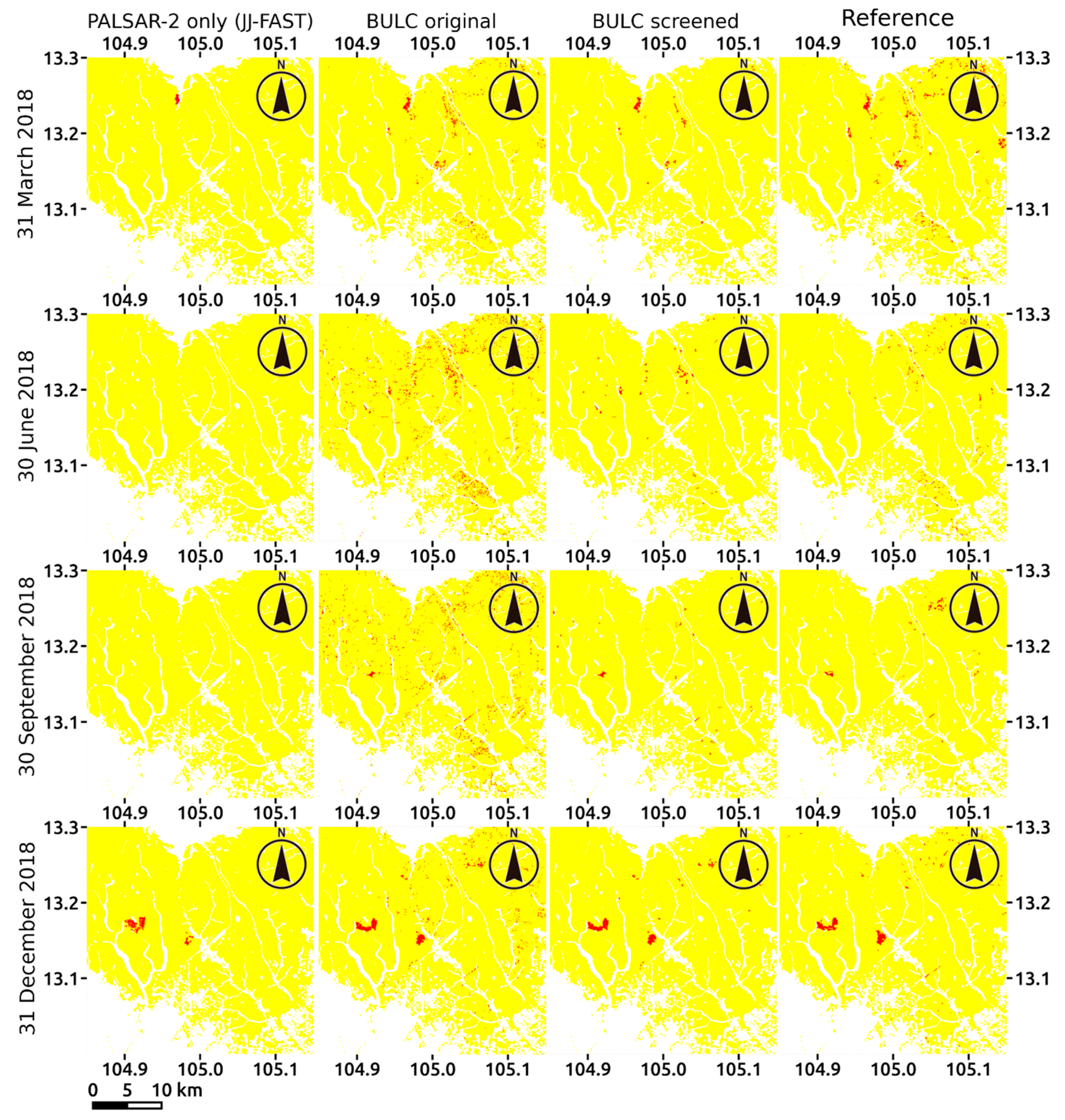
3.2. Effect of Sensor Integration

The most important effect of the sensor integration was improvement in the near-real-time properties of the algorithm. Figure 6 shows an example of the complementation of a cloud-covered area in Landsat by the other sensors. The omitted deforestation in Landsat (red area in Figure 6A) was successfully complemented mainly by PALSAR-2 (red area in Figure 6B), which is not affected by cloud cover. If we used only Landsat, then the deforestation area would not have been observed before the next time step, where a cloud-free observation was available.

From another point of view, the sensor integration significantly improved the PA most of the time compared with the Landsat-only detection (Figure 7). By contrast, the UA decreased when integrating PALSAR-2 and ASTER data (i.e., the commission error of deforestation was increased).

4. Discussion

4.1. Accuracy of the Integration Map

By using combined multiple satellite sensors (Landsat, ASTER and PALSAR-2), we created deforestation maps with better near-real-time properties. Indeed, the integration of the microwave sensor (PALSAR-2) complemented the observation gap of the optical sensors caused by cloud cover (Figure 6), which often occurs in tropical regions [18,19]. This feature is particularly important to provide an early warning of deforestation. This algorithm may also contribute to the prompt monitoring of sediment disasters in mountainous forests [49].

However, we sometimes detected small-scale fake deforestation with our algorithm, and this fake deforestation leads to the observation of less UA (i.e., more commission errors) after sensor integration, relative to the Landsat-only algorithm (Figure 7). These small commission errors can be attributed to (1) remnant cloud/cloud-shadow noise, even after double (i.e., preliminary QA check and SVM cloud mask) cloud screening of the optical sensors; (2) remnant speckle noise, even after the spatiotemporal smoothing of PALSAR-2; and (3) misclassification in the NN (also related to the previous two error sources). The NN suffered not only from (1) and (2) but also from a limited number of feature images and reforestation or greening effects in the areas where deforestation occurred. Unlike the simple one-time land-cover classification of the forest/barren areas, the classification of the never-deforested areas/ever-deforested areas is more challenging. The use of more sophisticated machine-learning approaches, such as convolutional NN [50], object-based classification [51], and algorithm improvement to describe reforestation, can mitigate the commission errors. Altered indices to be input into the NN may also change the classification accuracy. Due to the lack of SWIR bands (after 2008), we could not use MNDWI and NDSI for the ASTER data, which seems to be useful in distinguishing bare soil from forests [52]. The integration order of the multiple sensors also affects the BULC accuracy. We tested five cases in which the multiple sensors were randomly ordered at the same time step. The average OA values obtained during the integration period (2017–2018) for each case were: (94.48 ± 0.19)%, (94.50 ± 0.22)%, (94.40 ± 0.17)%, (94.46 ± 0.15)%, and (94.49 ± 0.25)%, which were all interior to the OA value achieved by our rule to determine the integration order (94.54% ± 0.16%). Thus, our proposed rule is the best one available so far, although a better method should be explored when applying our approach to another site.

Furthermore, the posterior probability derived from BULC can be used as a tunable threshold of deforestation. Original BULC (and Bayesian theorem) classifies a pixel as a class that indicates the highest posterior probability. This study uses only two (forest/deforestation) classes, where the threshold value of the posterior probability of deforestation can be interpreted as 0.5. When replaced with a higher value (e.g., 0.6) in 2017, we confirmed a suppression in deforestation detection and an improvement in the UA. Depending on user demand, more detailed flags referring to the posterior probability can be flexibly used, e.g., forest (0–0.3), suspicious region (0.3–0.7), and deforestation (0.7–1.0).

We also confirmed that applying the constraint of the posterior probability in BULC is important for avoiding the zero priors paradox [45,47]. With no constraints, more omissions of deforestation may occur as time passes. By contrast, excessive constraints may degrade the robustness of the algorithm against erroneous input data (Figure 5). Therefore, the range of the constraint should be carefully tuned in advance. An appropriately tuned constraint enabled us to mitigate errors (Figure 5), thereby contributing to the robustness of the overall algorithm. The BULC-based sensor fusion also overcame the limitation of the approach by Mizuochi et al. [24,25] because it is not dependent on any past match-ups but is the best-effort update of land cover using the Bayesian framework.

With the tuned constraint (0.95%–0.05%), the UA, PA, and OA of the deforestation (land-cover) map for the study period were 94.0% ± 4.5%, 80.0% ± 10.1%, and 96.4% ± 1.9%, respectively. Note that the estimated accuracy may contain uncertainties arising from errors in the reference maps: (1) uncertainties in the interpretation of different source images having different spatial resolutions and sensor mechanisms; (2) overlooking deforestation due to cloud contamination in the optical images, and (3) overlooking or commissioning deforestation due to human error, resulting in inevitable uncertainties in the reference maps that may lead to an underestimation of their accuracy. Efforts to create more accurate reference data based on more data sources (and if possible, based on in-situ surveys) should be continued.

4.2. Comparison with Other Algorithms

The map of Hansen et al. [12] was based on a simple machine-learning (bagged decision tree) algorithm solely using Landsat, whereas the map of JAXA was based on a time-series analysis that is similar to our time-series module solely using PALSAR-2. The comparison of our map with those single-sensor-based maps seemed beneficial in revealing the advantage of our algorithm and the effect of sensor integration.

Our algorithm showed accuracies comparable with (or even higher in the past) those of Hansen et al. [12] in the yearly time step (Figure 8). Moreover, although the algorithm only depended on a Landsat time-series analysis in the past period, it showed better PA, particularly for 2003–2014. This suggests that even only with Landsat, our time-series analysis could make fewer omissions than Hansen’s algorithm, which is also Landsat-dependent. In recent years, particularly in 2017 when the sensor integration was conducted, slightly less UA and PA were observed in our algorithm. Unfortunately, the algorithm of Hansen et al. [12] was not available for 2018 and later. Therefore, it was difficult to investigate whether this was a significant tendency. Overall, the UA, PA, and OA of the annual change-detection maps derived by our algorithm were (74.4 ± 12.3)%, (68.5 ± 9.8)%, and (97.8 ± 1.8)%, which seemed comparable or even superior to the product of Hansen et al. [12] (i.e., 70.3% ± 9.7%, 49.4% ± 21.5%, and 97.3% ± 2.2%, respectively).

Given that the product of JAXA adopted segment-base deforestation mapping, pixel-base accuracy assessment was not suitable. Instead, we compared the spatial pattern of the change detection between our maps and those of JAXA (Figure 9). In the JAXA algorithm, small (under 3 ha) deforestation patches were screened to eliminate the errors caused by sensor noise. For consistency, we also attempted to screen out deforestation patches under the specified area. Furthermore, the time step of JAXA’s product was not uniform, thus making it difficult to conduct a match-up every 1.5 months. Consequently, the comparison was performed with a longer time step (3 months).

Apparently, our maps were more consistent to the reference maps than the JAXA maps, which were only based on PALSAR-2. JAXA maps mostly had small (but over 3 ha) deforestation omissions and occasionally large omissions (e.g., in 30 September, 2018 in Figure 9), thereby suggesting that the integration of optical sensors with PALSAR-2 compensated for the relatively coarser spatial resolution and speckle-noise effect of PALSAR-2. This resulted in a more realistic detection of deforestation. On the contrary, erroneous small patches were detected in the original (i.e., not screened) BULC maps, particularly on 30 June and 30 September in 2018. The noise seemed to be treated by a screening method by the JAXA products. This suggests that post-processing, such as the screening of small deforestation patches, and expansion/contraction treatments may also be effective in improving the accuracy of the end result.

Another important aspect of our achieved product is the time step of detection. We created the maps every 1.5 months, which is more frequent than Hansen’s maps (i.e., yearly [12]) and comparably frequent to the maps of Reiche et al. [14] (with a mean time lag of 22 days). A similar detection frequency was also provided by the JAXA maps (every observation of PALSAR-2), although it featured a large portion of omitted deforestations (Figure 9). Fortunately, with the integrated use of optical images, such an omission was compensated in our algorithm. This flexibility of integrating different sensors is the advantage of the Bayesian approach. The sensor integration of Sentinel-1 and Sentinel-2 may help to further improve their accuracy and near-real-time properties but may not be straightforward, particularly for Sentinel-1, owing to their shorter penetration depths into the forest [27]. Future investigations on the applicability of our algorithm in other landscapes and on a global scale may also improve the current findings.

5. Conclusions

In this research, we demonstrated the flexibility of a sensor integration approach for automated deforestation mapping. The developed algorithm includes a time-series analysis with Landsat stacks and a multilayered NN with ASTER and PALSAR-2, followed by BULC. By using the algorithm, we were able to create deforestation maps with better accuracy than existing deforestation maps (products of Hansen et al. and JAXA) for every 1.5 months. This approach may contribute to the development of early-warning deforestation systems and prompt monitoring of sediment disasters in mountainous forests. We also investigated the effects of the constraint of posterior probability in the Bayesian approach. Our algorithm with the best-tuned constraint achieved 94.0% ± 4.5% for UA, 80.0% ± 10.1% for PA, and 96.4% ± 1.9% for OA in the deforestation maps, on average. Given the flexibility of the Bayesian approach, the integration of other long-term Earth observation data (including small satellites, airborne, and drone data) seems promising. Further investigations are needed on the application of our approach to such other sensor combinations and other landscapes.

References

- IPCC. Climate Change 2014: Mitigation of Climate Change; Contribution of Working Group III to the Fifth Assessment Report of the Intergovernmental Panel on Climate Change; Cambridge University Press: Cambridge, UK; New York, NY, USA, 2014. [Google Scholar]
- Giam, X. Global biodiversity loss from tropical deforestation. Proc. Natl. Acad. Sci. USA 2017, 114, 5775–5777. [Google Scholar] [CrossRef] [PubMed]
- Adikari, Y.; Noro, T. A Global Outlook of Sediment-Related Disasters in the Context of Water-Related Disasters. Int. J. Eros. Control Eng. 2010, 3, 110–116. [Google Scholar] [CrossRef][Green Version]
- Tranter, V. Food and Agriculture Organization of the United Nations; Cambridge University Press (CUP): Cambridge, UK, 2015; pp. 388–398. [Google Scholar]
- Espejo, J.C.; Messinger, M.; Román-Dañobeytia, F.; Ascorra, C.; Fernandez, L.E.; Silman, M. Deforestation and Forest Degradation Due to Gold Mining in the Peruvian Amazon: A 34-Year Perspective. Remote Sens. 2018, 10, 1903. [Google Scholar] [CrossRef]
- Potapov, P.; Turubanova, S.A.; Hansen, M.C.; Adusei, B.; Broich, M.; Altstatt, A.; Mane, L.; Justice, C.O. Quantifying forest cover loss in Democratic Republic of the Congo, 2000–2010. Remote Sens. Environ. 2012, 122, 106–116. [Google Scholar] [CrossRef]
- Stibig, H.J.; Achard, F.; Carboni, S.; Rasi, R.; Miettinen, J. Change in tropical forest cover of Southeast Asia from 1999 to 2010. Biogeoscience 2014, 11, 247–258. [Google Scholar] [CrossRef]
- Houghton, R.; Greenglass, N.; Baccini, A.; Cattaneo, A.; Goetz, S.; Kellndorfer, J.; Laporte, N.; Walker, W. The role of science in Reducing Emissions from Deforestation and Forest Degradation (REDD). Carbon Manag. 2010, 1, 253–259. [Google Scholar] [CrossRef]
- Hansen, M.; DeFries, R. Detecting long-term global forest change using continuous fields of tree-cover maps from 8-km Advanced Very High Resolution Radiometer (AVHRR) data for the years 1982–1999. Ecosystems 2004, 7, 695–716. [Google Scholar] [CrossRef]
- Potapov, P.; Hansen, M.C.; Stehman, S.V.; Loveland, T.R.; Pittman, K. Combining MODIS and Landsat imagery to estimate and map boreal forest cover loss. Remote Sens. Environ. 2008, 112, 3708–3719. [Google Scholar] [CrossRef]
- Huang, C.; Goward, S.N.; Masek, J.G.; Thomas, N.; Zhu, Z.; Vogelmann, J.E. An automated approach for reconstructing recent forest disturbance history using dense Landsat time series stacks. Remote Sens. Environ. 2010, 114, 183–198. [Google Scholar] [CrossRef]
- Hansen, M.C.; Potapov, P.V.; Moore, R.; Hancher, M.; Turubanova, S.A.; Tyukavina, A.; Thau, D.; Stehman, S.V.; Goetz, S.J.; Loveland, T.R.; et al. High-Resolution Global Maps of 21st-Century Forest Cover Change. Science 2013, 342, 850–853. [Google Scholar] [CrossRef]
- Mermoz, S.; Le Toan, T. Forest Disturbances and Regrowth Assessment Using ALOS PALSAR Data from 2007 to 2010 in Vietnam, Cambodia and Lao PDR. Remote Sens. 2016, 8, 217. [Google Scholar] [CrossRef]
- Reiche, J.; Hamunyela, E.; Verbesselt, J.; Hoekman, D.; Herold, M. Improving near-real time deforestation monitoring in tropical dry forests by combining dense Sentinel-1 time series with Landsat and ALOS-2 PALSAR-2. Remote Sens. Environ. 2018, 204, 147–161. [Google Scholar] [CrossRef]
- Marshak, C.; Simard, M.; Denbina, M. Monitoring Forest Loss in ALOS/PALSAR Time-Series with Superpixels. Remote Sens. 2019, 11, 556. [Google Scholar] [CrossRef]
- Hansen, M.C.; Krylov, A.; Tyukavina, A.; Potapov, P.V.; Turubanova, S.; Zutta, B.; Ifo, S.; Margono, B.; Stolle, F.; Moore, R. Humid tropical forest disturbance alerts using Landsat data. Environ. Res. Lett. 2016, 11, 34008. [Google Scholar] [CrossRef]
- JICA-JAXA Forest Early Warning System in the Tropics (JJ-FAST). Available online: https://www.eorc.jaxa.jp/jjfast/ (accessed on 8 May 2019).
- Ju, J.; Roy, D.P. The availability of cloud-free Landsat ETM+ data over the conterminous United States and globally. Remote Sens. Environ. 2008, 112, 1196–1211. [Google Scholar] [CrossRef]
- Olander, L.P.; Gibbs, H.K.; Steininger, M.; Swenson, J.J.; Murray, B.C. Reference scenarios for deforestation and forest degradation in support of REDD: A review of data and methods. Environ. Res. Lett. 2008, 3, 025011. [Google Scholar] [CrossRef]
- Omar, H.; Misman, M.A.; Kassim, A.R. Synergetic of PALSAR-2 and Sentinel-1A SAR polarimetry for retrieving aboveground biomass in dipterocarp forest in Malaysia. Appl. Sci. 2017, 7, 675. [Google Scholar] [CrossRef]
- Schwaller, M.; Hall, F.; Gao, F.; Masek, J. On the blending of the Landsat and MODIS surface reflectance: Predicting daily Landsat surface reflectance. IEEE Trans. Geosci. Remote Sens. 2006, 44, 2207–2218. [Google Scholar]
- Zhu, X.; Chen, J.; Gao, F.; Chen, X.; Masek, J.G. An enhanced spatial and temporal adaptive reflectance fusion model for complex heterogeneous regions. Remote Sens. Environ. 2010, 114, 2610–2623. [Google Scholar] [CrossRef]
- Belgiu, M.; Stein, A. Spatiotemporal Image Fusion in Remote Sensing. Remote Sens. 2019, 11, 818. [Google Scholar] [CrossRef]
- Mizuochi, H.; Hiyama, T.; Ohta, T.; Fujioka, Y.; Kambatuku, J.R.; Iijima, M.; Nasahara, K.N. Development and evaluation of a lookup-table-based approach to data fusion for seasonal wetlands monitoring: An integrated use of AMSR series, MODIS, and Landsat. Remote Sens. Environ. 2017, 199, 370–388. [Google Scholar] [CrossRef]
- Mizuochi, H.; Nishiyama, C.; Ridwansyah, I.; Nasahara, K.N. Monitoring of an Indonesian Tropical Wetland by Machine Learning-Based Data Fusion of Passive and Active Microwave Sensors. Remote Sens. 2018, 10, 1235. [Google Scholar] [CrossRef]
- Cardille, J.A.; Fortin, J.A. Bayesian updating of land-cover estimates in a data-rich environment. Remote Sens. Environ. 2016, 186, 234–249. [Google Scholar] [CrossRef]
- White, L.; Brisco, B.; Dabboor, M.; Schmitt, A.; Pratt, A. A Collection of SAR Methodologies for Monitoring Wetlands. Remote Sens. 2015, 7, 7615–7645. [Google Scholar] [CrossRef]
- Gorelick, N.; Hancher, M.; Dixon, M.; Ilyushchenko, S.; Thau, D.; Moore, R. Google Earth Engine: Planetary-scale geospatial analysis for everyone. Remote Sens. Environ. 2017, 202, 18–27. [Google Scholar] [CrossRef]
- Vogelmann, E.J.; Helder, D.; Morfitt, R.; Choate, M.J.; Merchant, J.W.; Bulley, H. Effects of Landsat 5 Thematic Mapper and Landsat 7 Enhanced Thematic Mapper Plus radiometric and geometric calibrations and corrections on landscape characterization. Remote Sens. Environ. 2001, 78, 55–70. [Google Scholar] [CrossRef]
- Li, P.; Jiang, L.; Feng, Z. Cross-comparison of vegetation indices derived from landsat-7 enhanced thematic mapper plus (ETM+) and landsat-8 operational land imager (OLI) sensors. Remote Sens. 2013, 6, 310–329. [Google Scholar] [CrossRef]
- Rouse, J.W.; Haas, R.H.; Schell, J.A.; Deering, D.W. Monitoring Vegetation Systems in the Great Plains with ERTS. In Proceedings of the 3rd ERTS Symposium, Washington, DC, USA, 10–14 December 1973; pp. 309–317. [Google Scholar]
- Xu, H. Modification of normalized difference water index (NDWI) to enhance open water features in remotely sensed imagery. Int. J. Remote Sens. 2006, 27, 3025–3033. [Google Scholar] [CrossRef]
- Faraklioti, M.; Petrou, M. Illumination invariant unmixing of sets of mixed pixels. IEEE Trans. Geosci. Remote Sens. 2001, 39, 2227–2234. [Google Scholar] [CrossRef]
- Koutsias, N.; Karteris, M.; Chuvieco, E. The use of intensity-hue-saturation transformation of landsat5 thematic mapper data for burned land mapping. Photogramm. Eng. Remote Sensing. 2000, 66, 829–839. [Google Scholar]
- METI AIST Satellite Data Archive System (MADAS). Available online: https://gbank.gsj.jp/madas/ (accessed on 8 May 2019).
- McFeeters, S.K. The use of the Normalized Difference Water Index (NDWI) in the delineation of open water features. Int. J. Remote Sens. 1996, 17, 1425–1432. [Google Scholar] [CrossRef]
- Falkowski, M.J.; Gessler, P.E.; Morgan, P.; Hudak, A.T.; Smith, A.M. Characterizing and mapping forest fire fuels using ASTER imagery and gradient modeling. For. Ecol. Manag. 2005, 217, 129–146. [Google Scholar] [CrossRef]
- Motohka, T.; Isoguchi, O.; Sakashita, M.; Shimada, M. Results of ALOS-2 PALSAR-2 Calibration and Validation after 3 Years of Operation. In Proceedings of the International Geoscience and Remote Sensing Symposium, Valencia, Spain, 25 July 2018. [Google Scholar]
- Pour, A.B.; Hashim, M. Application of Landsat-8 and ALOS-2 data for structural and landslide hazard mapping in Kalimantan, Malaysia. Nat. Hazards Earth Syst. Sci. 2017, 17, 1285–1303. [Google Scholar] [CrossRef]
- Thapa, R.B.; Watanabe, M.; Motohka, T.; Shimada, M. Potential of high-resolution ALOS–PALSAR mosaic texture for aboveground forest carbon tracking in tropical region. Remote Sens. Environ. 2015, 160, 122–133. [Google Scholar] [CrossRef]
- Foroosh, H.; Zerubia, J.; Berthod, M. Extension of phase correlation to subpixel registration. IEEE Trans. Image Process. 2002, 11, 188–200. [Google Scholar] [CrossRef]
- Olofsson, P.; Foody, G.M.; Herold, M.; Stehman, S.V.; Woodcock, C.E.; Wulder, M.A. Good practices for estimating area and assessing accuracy of land change. Remote Sens. Environ. 2014, 148, 42–57. [Google Scholar] [CrossRef]
- Bishop, C.M. Pattern Recognition and Machine Learning; Springer: New York, NY, USA, 2006. [Google Scholar]
- Kikuchi, M.; Yoshida, M.; Okabe, M.; Umemura, K. Confidence Interval of Probability Estimator of Laplace Smoothing. In Proceedings of the 2015 2nd International Conference on Advanced Informatics: Concepts, Theory and Applications (ICAICTA), Chonburi, Thailand, 19–22 August 2015; pp. 1–6. [Google Scholar]
- Basieva, I.; Pothos, E.; Trueblood, J.; Khrennikov, A.; Busemeyer, J. Quantum probability updating from zero priors (by-passing Cromwell’s rule). J. Math. Psychol. 2017, 77, 58–69. [Google Scholar] [CrossRef]
- Jackman, S. Bayesian Analysis for the Social Sciences; John Wiley & Sons: Hoboken, NJ, USA, 2009; pp. 18–19. [Google Scholar]
- Fortin, J.A.; Cardille, J.A.; Perez, E. Multi-sensor detection of forest-cover change across 45 years in Mato Grosso, Brazil. Remote Sens. Environ. 2019, 111266. [Google Scholar] [CrossRef]
- Stehman, S.V. Estimating area and map accuracy for stratified random sampling when the strata are different from the map classes. Int. J. Remote Sens. 2014, 35, 4923–4939. [Google Scholar] [CrossRef]
- Nakano, Y.; Yamakoshi, T.; Shimizu, T.; Tamura, K.; Doshida, S. The Evaluation of Eruption Induced Sediment Related Disasters using Satellite Remote Sensing-Applications for Emergency Response. Int. J. Eros. Control Eng. 2010, 3, 34–42. [Google Scholar] [CrossRef][Green Version]
- Holloway, J.; Mengersen, K. Statistical Machine Learning Methods and Remote Sensing for Sustainable Development Goals: A Review. Remote Sens. 2018, 10, 1365. [Google Scholar] [CrossRef]
- Xie, Z.; Roberts, C.; Johnson, B. Object-based target search using remotely sensed data: A case study in detecting invasive exotic Australian Pine in south Florida. ISPRS J. Photogramm. Remote Sens. 2008, 63, 647–660. [Google Scholar] [CrossRef]
- Jin, Y.; Sung, S.; Lee, D.K.; Biging, G.S.; Jeong, S. Mapping Deforestation in North Korea Using Phenology-Based Multi-Index and Random Forest. Remote Sens. 2016, 8, 997. [Google Scholar] [CrossRef]