Article

Retrieval of Cloud Optical Thickness from Sky-View Camera Images using a Deep Convolutional Neural Network based on Three-Dimensional Radiative Transfer

1
Graduate School of Science, Tohoku University, Sendai, Miyagi 980-8578, Japan
2
Department of Atmospheric and Oceanic Sciences, University of Colorado, Boulder, CO 80309-0311, USA
3
Laboratory for Atmospheric and Space Physics, University of Colorado, Boulder, CO 80303-7814, USA
4
Center for Environmental Remote Sensing, Chiba University, Chiba 263-8522, Japan
5
Meteorological Research Institute, Japan Meteorological Agency, Tsukuba 305-0052, Japan
*
Author to whom correspondence should be addressed.
Remote Sens. 2019, 11(17), 1962; https://doi.org/10.3390/rs11171962
Submission received: 2 July 2019 / Revised: 13 August 2019 / Accepted: 17 August 2019 / Published: 21 August 2019

Abstract

:
Observation of the spatial distribution of cloud optical thickness (COT) is useful for the prediction and diagnosis of photovoltaic power generation. However, there is not a one-to-one relationship between transmitted radiance and COT (so-called COT ambiguity), and it is difficult to estimate COT because of three-dimensional (3D) radiative transfer effects. We propose a method to train a convolutional neural network (CNN) based on a 3D radiative transfer model, which enables the quick estimation of the slant-column COT (SCOT) distribution from the image of a ground-mounted radiometrically calibrated digital camera. The CNN retrieves the SCOT spatial distribution using spectral features and spatial contexts. An evaluation of the method using synthetic data shows a high accuracy with a mean absolute percentage error of 18% in the SCOT range of 1–100, greatly reducing the influence of the 3D radiative effect. As an initial analysis result, COT is estimated from a sky image taken by a digital camera, and a high correlation is shown with the effective COT estimated using a pyranometer. The discrepancy between the two is reasonable, considering the difference in the size of the field of view, the space–time averaging method, and the 3D radiative effect.

Graphical Abstract

1. Introduction

Clouds primarily modulate the Earth's energy balance and climate. The observation of the spatial distribution of cloud physical properties, in particular, cloud optical thickness (COT), is useful for the evaluation of clouds’ radiative effects and the diagnosis of photovoltaics, which is a promising form of renewable energy [1]. Many methods for the estimation of COT by optical measurement from satellites and the ground have been developed. Satellite remote sensing often relies on the reflection of solar radiation, while ground-based remote sensing usually relies on transmission. A one-to-one relationship between transmitted radiance and COT does not hold (COT ambiguity), and it is difficult to estimate COT from transmitted radiance measured at a single wavelength. Therefore, many ground-based remote sensing methods combining multiple wavelengths have been proposed. For example, Marshak et al. [2] and Chiu et al. [3] estimated COT using differences in the transmitted radiances between two wavelengths over a vegetated surface. Kikuchi et al. [4] estimated COT using the difference between the transmission at water-absorbing and non-absorbing bands. McBride et al. [5] estimated COT using the spectral gradient of transmitted radiance in the near-infrared and shortwave infrared. Niple et al. [6] estimated COT using the equivalent width of the oxygen absorption band. In these methods, the COT in the zenith direction is estimated using the transmitted radiance in the zenith direction. However, for the evaluation of the amount of photovoltaic power generation, it is desirable to estimate the COT distribution in the whole sky. Therefore, the use of digital cameras is attractive. Mejia et al. [7] developed the radiance red-to-blue ratio (RRBR) method, which combines the ratio of the transmitted radiance of the red and blue channels (red-to-blue ratio; RBR) and the transmitted radiance of the red channel. They estimated the COT of each pixel from a camera image.
Conventional cloud remote sensing methods, including all of the above-mentioned methods, perform the estimation based on a one-dimensional (1D) radiative transfer model that assumes plane-parallel clouds. In the case of satellite observation, information on the spatial arrangement of cloud water is usually recorded as a two-dimensional (2D) image. The estimation method based on a 1D radiative transfer model implicitly assumes the independent pixel approximation (IPA) [8], which requires each pixel to be independent of its spatial context. However, in the presence of broken clouds, the effects of the horizontal transport of radiation—in other words, the three-dimensional (3D) radiative effect—are very large. Many studies have revealed that 3D radiative effects cause large errors in the estimation of cloud physical quantity if the IPA is assumed [9,10,11,12,13]. The observed radiance is influenced not only by the characteristics of the cloud elements along the line of sight, but also by the 3D arrangement of the cloud water around the line of sight. Thus, to accurately estimate the characteristics of the clouds, a cloud estimation method should take the 3D arrangement of the clouds into account. The multi-pixel method is expected to be effective in estimating cloud properties using multiple pixels, including the neighboring pixels of the target pixel [14]. Therefore, the use of a neural network (NN) that is trained based on 3D radiative transfer calculation is promising in practical applications. Such NN cloud retrieval methods started with the feasibility studies of the multi-spectral multi-pixel method by Faure et al. [15,16], and have been extended to practical applications to analyze Moderate-resolution Imaging Spectroradiometer (MODIS) observational data by Cornet et al. [17,18]. In the method of Cornet et al. [17,18], the input data were radiances from a small image area of about 1 × 1 km2. They estimated bulk properties such as the average and degree of heterogeneity of COT and cloud droplet effective radius (CDER), and the cloud fraction. Evans et al. [19] tested an NN to estimate COT, using spatial features of multi-directional observation images at visible wavelengths. In recent years, deep learning techniques to train deep NNs have emerged, which enables applications involving large, complicated problems of estimation, detection, classification, and prediction. As a result of its very high modeling ability, deep learning has rapidly grown in popularity for various remote sensing applications. Okamura et al. [20] trained a deep convolutional neural network (CNN) based on 3D radiative transfer, and estimated COT and CDER simultaneously at multiple pixels of a multi-spectral image used as input. They showed that the CNN achieved a high accuracy and efficient estimation.
On the other hand, the 3D radiative effects on the transmitted radiance observed on the ground are not well understood, and their influence on the retrieval of the cloud physical properties from ground-based observation is not clear. For transmitted radiance, radiation enhancement frequently occurs [21]. Several algorithms have been proposed to estimate the 3D cloud field by iterative 3D radiative transfer calculations, using the variational and ensemble Kalman filter methods [22,23,24,25,26,27]. However, their computational cost is high, as they perform multiple computationally heavy calculations of 3D radiative transfer, and gradients are needed in the variational methods. The purpose of this study is to develop a practical, efficient (fast and accurate) method that can be applied for the estimation of the spatial distribution of COT from images actually taken by a ground-based digital camera. Following the previous work by Okamura et al. [20], we have trained deep CNNs based on a 3D radiative transfer model. Although the prior work [20] showed the feasibility of deep learning-based cloud retrieval, the conditions of cloud, atmosphere, and surface were idealized and limited. In this study, synthetic data are generated with more variety of cloud, atmosphere, and surface conditions. In addition, we have explored several kinds of new DNN architecture and techniques recently available in the literature, in order to achieve accuracy and computational efficiency.
This paper is organized as follows. Section 2 describes the cloud data and radiative transfer model calculations. Section 3 presents an investigation of the 3D radiative effects on transmitted zenith radiance, and tests how NN and CNN help to overcome the COT ambiguity and 3D radiative effects. Section 4 presents a deep CNN model that estimates COT from sky-view camera images, with accuracy evaluation by synthetic data. In Section 5, the CNN is applied to actual observations from a digital camera, and the CNN retrieval is compared with COT estimated using a pyranometer. A summary and conclusions are given in Section 6.

2. Data and Methods

A large amount of synthetic data were generated by simulations using a high-resolution cloud model and a 3D radiative transfer model, and the synthetic data were used for training and testing the NN and CNN models.

2.1. SCALE-LES Cloud-Field Data

In this study, we used high-resolution cloud data reproduced by the Scalable Computing for Advanced Library and Environment-Large Eddy Simulation (SCALE-LES) model [28,29,30]. Three kinds of simulation datasets were used, namely, an open-cell case with a low concentration of cloud condensation nuclei (clean), a closed-cell case with a high concentration (polluted), and a Barbados Oceanographic and Meteorological Experiment (BOMEX) case reproducing convective clouds in the tropics. Each case has 60 time-steps with 10-minute intervals. Spatially-coarsened grid data were used in this study. The open- and closed-cell cases cover a horizontal area of 28 × 28 km2 with a horizontal resolution (∆x and ∆y) of 0.14 km. The vertical resolution is higher for the lower atmosphere (∆z = 0.04 km at the lower end) and decreases with increasing height, and ∆z = 0.2 km at the top of the model domain. The BOMEX case covers a horizontal area of 7.2 × 6.4 km2, with a horizontal resolution (∆x and ∆y) of 0.05 km and a vertical resolution of ∆z = 0.04 km. In all cases, the lateral boundary conditions are periodic.
SCALE-LES uses a double-moment bulk microphysics scheme to obtain the liquid water content (LWC) and cloud particle number density (N). The two quantities are converted to optical properties for radiative transfer calculations. COT at 550 nm is defined as follows:
τ c = 0 β e x t ( z ) d z
where z is the height and β e x t is the volume extinction coefficient of the cloud particles, as follows:
β e x t = Q e x t 3 w 4 π ρ w r e
where Q e x t is the extinction efficiency factor, w is the LWC, ρ w is the droplet internal density, and r e is the CDER. In this study, we assume only water clouds. r e is determined by the following:
r e = ( 3 w 4 π ρ w N χ ) 1 / 3
where χ is a parameter determined by the particle size distribution. As the particle size distribution is assumed to be a lognormal distribution in this study, χ can be obtained from the geometrical standard deviation, s, by the following equation:
χ = exp ( 3 × ln 2 s )
Figure 1 shows examples of snapshots of cloud fields. In the closed-cell case, optically-thick clouds cover almost the whole sky, and are relatively homogeneous in the horizontal directions. In the open case, stratocumulus clouds with small gaps are distributed. In the BOMEX case, cumulus clouds are sparsely distributed. Temporal variations of cloud physical properties, including a horizontal heterogeneity index defined in Equation (A1), in the three cases are presented in Figure A1.

2.2. Simulations of Spectral Radiance

The Monte Carlo Atmospheric Radiative Transfer Simulator (MCARaTS) [31,32], a 3D atmospheric radiative transfer model, is used to generate synthetic images of a ground-based camera. This model uses the Monte Carlo method and ray-tracing to track the trajectory of the model photons, and calculates the spectral radiances for arbitrary locations and directions. The model inputs are the 3D distributions of the atmospheric optical characteristics of every wavelength and ground surface albedo. The model atmosphere up to 50 km is divided into approximately 50 layers, and the 3D distribution of the clouds obtained from SCALE-LES is incorporated into the troposphere. The cloud fields are modified from the original SCALE-LES simulations in various ways, so as to increase the variety of cases. For example, cloud optical properties can be modified by scaling and adding bias. Rayleigh scattering by air molecules, absorption by ozone, and scattering by cloud particles are considered. The single scattering albedo and the scattering phase function, depending on the wavelength and CDER, are calculated using the Lorenz–Mie theory. The visible-wavelength range of 385–715 nm is divided into 11 wavelength bands with a width of 30 nm, and the average spectral radiance of each wavelength band is calculated. Furthermore, in this study, the spectral response functions of a digital camera (described later in Section 5) are used to convert the 11-band spectral radiances to those of red/green/blue (RGB) channels. More details of the synthetic image generation are presented in Section 3 and Section 4.

3. Test of COT Retrieval from Zenith Transmittance

In this section, in order to understand the elements for COT estimation with high accuracy from transmitted visible radiation, we tested various algorithms for limited cases. Previous studies suggest that retrieval algorithms should be based on a 3D radiative transfer model, and use multiple pixels including surrounding pixels [14,15,20]. Contributions to accuracy improvement are evaluated by comparing several estimation algorithms, including the RRBR method [7].

3.1. 3D Radiative Effects in Zenith Transmittance

First, we investigated the relationship between COT and transmitted radiance in order to understand how the 3D radiative effect works. The horizontal distributions of the visible transmitted radiance in the zenith direction are calculated by 3D radiative transfer and the IPA, respectively, for the BOMEX case, as shown in Figure 2. Compared to IPA radiance, the sun-side of a cloud is bright and the opposite side is dark in the 3D radiance, which are the effects of radiation enhancement and shading, respectively. These cannot be expressed in the IPA calculation, because the radiative transfer calculation is performed for each air column independently. Interestingly, comparing the RBR of the 3D calculation with the IPA, the 3D scene is redder in parts where radiation enhancement appears, and bluer in the shadowed parts. Therefore, 3D effects change the spectral slope in the visible region, and make the scene with broken clouds more colorful.
Figure 3 shows the relationship between the red-channel radiance and the RBR, and the column COT for each pixel for the example shown in Figure 2. The IPA radiance is determined from the column COT, and has a peak at a COT of about 5. The radiance increases with the increasing COT when COT <5, and decreases with the increasing COT when COT >5. Therefore, COT has two solutions for the same IPA radiance value (COT ambiguity), and COT cannot be estimated using a single wavelength. As shown by Mejia et al. [7], it is possible to distinguish whether a cloud is optically thin or thick by using RBR. However, this solution is effective only for homogeneous clouds assuming the IPA, and is not effective for broken clouds, because the 3D radiative effect perturbs the spectral signature of thin vs. thick clouds beyond its usefulness. Even though the spectral information cannot be used to resolve the COT ambiguity in the case of strong 3D effects, the correct COT can be still be retrieved based on structural context. As 3D radiance depends on the spatial arrangement of the nearby cloud elements, this should be taken into consideration in the retrieval of COT.

3.2. Data Generation

For the tests of various NN/CNNs for COT estimation, the synthetic data of the transmitted zenith radiance are generated by radiative transfer simulations. Only the BOMEX case was used for this purpose. For simplicity, the solar zenith and azimuth angles (SZA and SAA, respectively) were fixed at 60° and 0°, respectively; the aerosol was assumed to be a rural model [33] with an optical thickness of 0.2; and the cloud base height was set at 500 m. In order to increase the variety of the cloud field, the original values of COT were modified by a randomly chosen factor between 0.2 and 5, and the cloud geometrical thickness was scaled by a factor of 0.5, 1.0, or 2.0. IPA and 3D radiative transfer calculations were performed, and the horizontal distribution of the band-mean radiances at RGB channels were calculated for the transmitted zenith radiance at ground level. The horizontal resolution is ∆x = ∆y = 0.05 km, and a radiance distribution can be obtained for 128 × 128 pixels per scene. Nine image patches with a size of 52 × 52 pixels were extracted from each scene. The green square in Figure 2 corresponds to one of these nine image patches, as an example. A total of 972 and 108 image patches were generated for the training and performance tests, respectively.

3.3. Design and Configuration of NN and CNN Models

The NNs and CNN listed in Table 1 were tested. All of the models were trained with the radiance of 3D and IPA calculations, respectively, as input data. Only 3D radiance data were used for error evaluation. RGB radiances are normalized by dividing by 800 W m−2 sr−1 µm−1 in the preprocessing, which makes it easy to train the neural network model. The model output is the non-linear transform of COT, as defined by the following:
τ c = H ( log 10 τ c + 1 ) × ( log 10 τ c + 1 ) / 3
where H is the Heaviside step function. The datasets used for training and evaluation were the same for all of the models, although the numbers of pixels in the input and output data were different among the models. NN-0 is an NN that uses the single-pixel radiance to estimate single-pixel COT, while NN-1 to NN-10 are the NNs that use multi-pixel radiances to estimate the COT at a central pixel. NN-M (M = 1–10) takes (2M + 1)2 pixels as an input, assuming that the size of one side of the peripheral area is M pixels. Each NN is a multi-layer perceptron model with a single middle layer. The number of nodes in each NN model was determined so that the degree of freedom of the model increased according to the complexity of the problem. In the training stage, the output pixels of the NN model were sampled one by one from 32 × 32 pixels centered on the image patch with a size of 52 × 52 pixels, and the corresponding input pixels included the radiance data of the surrounding pixels when M >0.
Among the models listed in Table 1, only the CNN model estimates COT at multiple pixels in a single operation. The input and output of the CNN are the radiances and COT, respectively, for the 52 × 52-pixel area, and the error evaluation is performed for the central 32 × 32 pixels, consistently with models NN-1 to NN-10. Therefore, in the CNN, the COT at the evaluated pixel is estimated using the radiances of 10 or more surrounding pixels. The structure of the CNN is shown in Figure 4. The basic structure was designed based on a pyramid scene network (PSPNet) [34]. In the forward calculation of CNN, the data are continuously processed through several layers, in which multi-channel convolution and non-linear transformation are performed. In the convolution layer, the output (uijm) of the mth output channel and pixel indices i and j is represented as follows:
u i j m = k = 0 K 1 p = 0 L 1 q = 0 L 1 z i + p , j + q , k h p q k m + b m
where zijk is the input signal of the kth input channel, h is the weight of an L × L convolution filter, and b is the bias. The convolution operation produces an output image (feature map) that responds to patterns similar to the filter patterns, combining spectral and spatial information contained in the input multi-channel image (feature map). The filter weight and bias coefficients are optimized in the training. The dashed lines in Figure 4 represent the so-called shortcuts; the detailed structure of the units with the shortcut is shown in the upper right of Figure 4. This unit with the shortcut is called a residual unit [35], which adds the input of the unit to the data obtained by the process involving multiple convolution operations. In general, the use of residual units facilitates the training of recent deeper networks. The processing order in a residual unit is based on the work of He et al. [36], and Zagoruyko and Komodakis [37]. In order to improve the regularization and generalization performance, the CNN uses batch normalization and dropout (with a fraction of 10%) [38,39]. The rectified linear function (ReLU) is also used in the residual unit. Batch normalization and ReLU are applied not only in residual units, but also after all convolution operations. PSPNet has multiple pooling layers with different scales, in which the feature maps are subsampled to coarse grids by averaging. In this study, four kinds of averaging poolings, with feature map sizes of 1 × 1, 2 × 2, 4 × 4, and 8 × 8, were used. Thus, it is expected that cloud spatial structures and 3D radiative effects at various horizontal scales can be learned. The number of output channels from each pooling layer is reduced to a quarter, and the feature map of each channel is enlarged (upsampled) by bilinear interpolation. Subsequently, the data from all of the pooling layers are concatenated along the channel dimension. Finally, multi-scale features are fused to obtain an image with the same size as the input image by the transposed convolution. The details of these deep NN techniques are summarized by Goodfellow et al. [39].
Adaptive moment estimation (Adam) [40] was used for training, that is, the optimization of the model parameters. The loss function to be minimized during training is the mean squared error of the COT transform in Equation (6). During the training, data samples are randomly rearranged and divided into mini-batches. For each mini-batch, a gradient calculation is performed and the model parameters are updated, and this process is iterated for all of the mini-batches. One epoch corresponds to the process for all of the data samples, and the optimization is continued for multiple epochs while shuffling data samples for each epoch [39]. The training of the NN models took between 3 and 5 hours for 500 epochs, while the training of the CNN took only 0.35 hours for 2000 epochs. As CNNs can obtain a result for multiple pixels simultaneously with a single operation, the calculation time required to process the same amount of data is significantly shorter than in the NN models. The NN model was implemented using the Chainer deep learning framework [41].

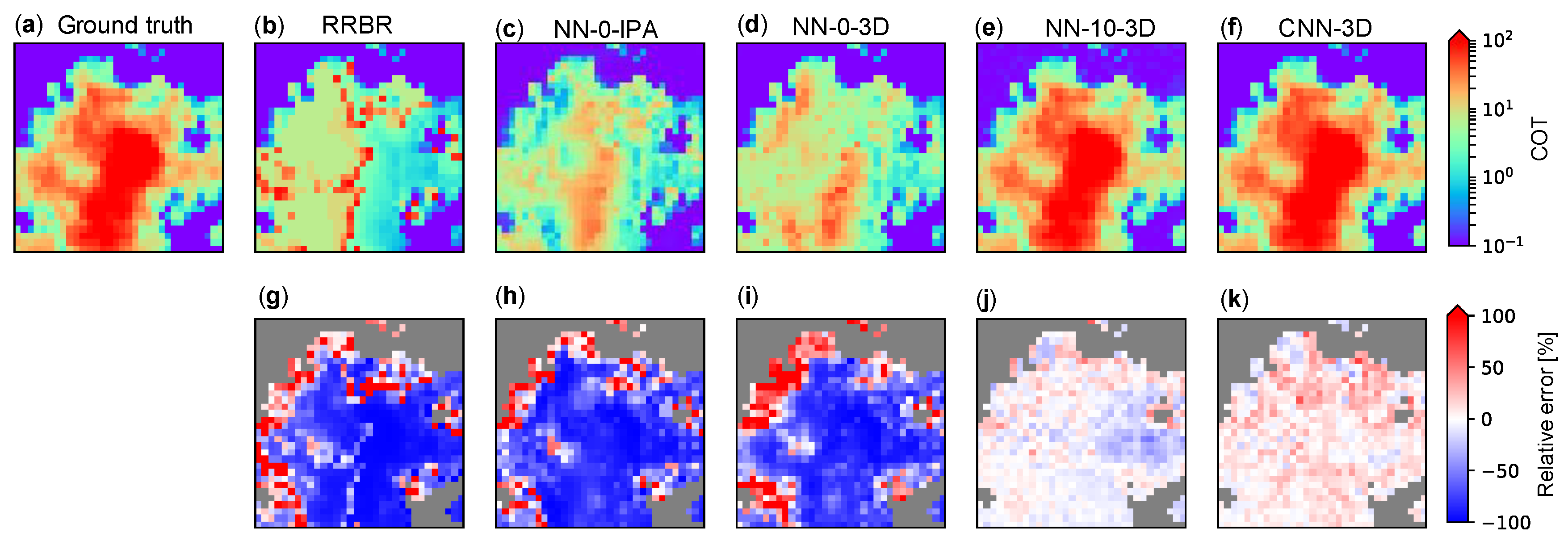
3.4. Comparison of Various NNs

Figure 5 shows an example of the estimation results using the RRBR method, NN-0-IPA, NN-0-3D, NN-10-3D, and CNN-3D. The RRBR method, NN-0-IPA, and NN-0-3D use the data of a single pixel as input. NN-0-IPA is considered to be a traditional IPA-based single-pixel estimation method implemented by NN, and NN-0-3D is a single-pixel estimation method trained by 3D radiances. As shown in Figure 3, NN-0-IPA and NN-0-3D are trained using very different radiances. The image patches shown in Figure 5 correspond to the red squares in Figure 2, and the illumination and shadowing effects work strongly on the sun side and the opposite side, respectively, of a large cumulus cloud. The estimation error is very large in the single-pixel retrieval methods (RRBR method, NN-0-IPA, and NN-0-3D). As the estimation error of NN-0-3D is as large as that of NN-0-IPA, COT cannot be accurately estimated from only the information at a single pixel, even if the NN is trained using the radiance data including 3D radiative effects. On the other hand, the estimation accuracy of NN-10-3D and CNN-3D, in which the horizontal distribution of the radiance of multiple pixels is used as the input, is dramatically improved. This can be ascribed to the fact that 3D radiative effects are well captured by considering the arrangement of the surrounding cloud elements.
The relative error of the COT estimated by each model is shown in Figure 6. The root-mean-square percentage error (RMSPE) is calculated by the following:
RMSPE = 1 n k = 1 n ϵ j 2
where ϵ j is the relative error (in %) of jth pixel sample, as follows:
ϵ = 100 × τ s c , e s t τ s c , t r u τ s c , t r u
where τ s c , e s t and τ s c , t r u represent the estimated and ground-based COTs, respectively. The single-pixel methods (RRBR and NN-0-IPA) based on the IPA tend to overestimate the COT for a COT of around 3, and underestimate COT for a COT of 10 or more. As clearly illustrated in Figure 3, the 3D radiance at a COT of ~5 or more is significantly larger than the IPA radiance by the illumination effect, and is close to the IPA radiance for a COT of 5. Thus, the IPA-estimated COT tends to be around 5, when the true COT is 5 or more. The IPA estimation is not improved by training, even when the surrounding pixels are included in the input. However, if an NN is trained based on the 3D radiance at multiple pixels, the estimation accuracy is improved. This is evident even in NN-1-3D (Figure 6c), which uses only eight adjacent pixels. Furthermore, it can be seen that the accuracy improves dramatically as the number of surrounding pixels increases (with increasing M).
Figure 7 shows the COT estimation accuracy of models NN-1 to NN-10, which verifies that the information of distant pixels is useful for COT estimation. This confirms that the estimation error decreases as the spatial scale of the input data increases. Figure 7 shows the results for only up to 10 pixels away from the center, that is, 500 m away, but it is expected that the estimation accuracy can be further improved by further expanding the spatial scale. It is known that the 3D radiative effect works mainly for a horizontal scale of up to about 5 km for clouds with a geometrical thickness of 500 m [14,42]. Figure 7 also shows the estimation error of CNN for comparison. The CNN model has the same estimation error as NN-6 or NN-7. However, as mentioned above, the operation of the CNN model is overwhelmingly fast, because it estimates the cloud properties of many pixels simultaneously. It can be seen from Table 1 that the CNN-3D model takes significantly less time to be trained (about 7% of the training time of NN-10-3D). This numerical advantage of the CNN-3D model becomes more important as the number of input and output pixels increase.

4. COT Retrieval from Synthetic Sky-View Camera Images

Based on the results in the previous section, a new CNN model was developed for COT retrieval from a sky-view camera image. The training was based on a large number of synthetic camera images that were simulated by 3D radiative transfer calculations.

4.1. Data Generation

In order to develop a practical estimation model, it is necessary to include various cloud fields, and various aerosol and underlying surface conditions in the training data. Therefore, the clouds, aerosols, and surface albedo were varied regularly or randomly in the simulations. By changing the LWC and cloud particle number density, the cloud extinction coefficient and CDER were modified from the original states. The cloud extinction coefficient was randomly modified by a factor within the range of 0.2–5. The cloud base height was set as 500, 1500, 2500, 3500, or 4500 m. The geometrical characteristics of the 3D clouds were modified by stretching or shrinking in the horizontal and vertical directions. The cloud geometrical thickness was changed by a factor of 0.5, 1, or 2, and the entire domain was stretched horizontally by a random factor within the range of 0.5–2 in the x and y directions of the Cartesian coordinate system. The rural type of aerosol was assumed as in the previous section, and the aerosol optical thickness was chosen randomly within the range of 0.04–1. The surface albedo was randomly chosen within the range of 0.02–0.5. The solar position was also random, with a solar zenith angle of 0–70° and a solar azimuth angle of 0–360°.
The synthetic camera image is generated by an image projection of the angular distribution of the spectral radiance within a field of view of the camera. The technical details of the camera used in this study are presented in Section 5.1. MCARaTS allows for the position, attitude, and viewing angle of the camera to be set arbitrarily. The horizontal location of the camera was random within the computational domain, and the camera was assumed to be oriented to the zenith. Each camera image was projected in an equidistant projection with a size of 128 × 128 pixels, with a diagonal angle of view of about 127° and a field of view within 45° of the image center in the vertical and horizontal axes of the image. The spectral radiance was calculated for the pixels, with a viewing zenith angle (VZA) of less than 45°. An example of the multi-directional lines of sight seen from a camera is schematically shown in Figure 1b. Because of the presence of Monte Carlo noise in the simulations, each of the RGB channels contains an average calculation noise of about 2%–4% at the pixel level.
An example of the input and output data of the CNN is shown in Figure 8. The input includes RGB radiances normalized by dividing by 800 W m−2 sr−1 µm−1 in the preprocessing, as in Section 3. As the observed radiance is strongly affected by the solar position, an additional channel in the CNN input represents the solar position. The solar position channel was represented by an isotropic 2D Gaussian distribution with a peak in the solar direction and a standard deviation of 50 pixels. A cloud property that is to be estimated from the camera images is the slant-column COT (SCOT) along the line of sight, corresponding to each pixel as follows:
τ s c = 0 β e x t ( s ) d s
where s is the distance from the camera. SCOT is calculated by ray-tracing using MCARaTS. The output of the CNN is actually the non-linear transform of SCOT, as follows:
τ s c = H ( log 10 τ s c + 1 ) × ( log 10 τ s c + 1 ) / 3
SCOT can be inverted from Equation (11), in which pixels with a SCOT <0.1 are reset as clear sky (i.e., SCOT = 0). The SCOT corresponding to a direction with the zenith angle θ can be converted into an equivalent COT (i.e., vertical integral of extinction) as in Equation (1), using the following equation:
τ c , e q ( θ ) = τ s c ( θ ) cos θ
A total of 115,200 samples were generated. These samples were divided into 103,680 samples for training and 11,520 samples for accuracy evaluation.

4.2. Design and Configuration of CNN Model

Figure 9 shows the structure of the CNN. The basic structure is the same as in Figure 4, but the input and output of the CNN in Figure 9 are images with a size of 128 × 128 pixels. The use of many layers generally increases the representation capability of the CNN model. The CNN in Figure 9 contains additional dilated convolution layers [43,44]. The dilated convolution can capture variation with a larger spatial scale, by widening the sampling interval of the convolution filter. The implementation of the dilated convolution into the residual unit is based on the work of Yu et al. [45]. The multiscale pooling layers facilitate to capture the local and global features, and they are fused by concatenation.
In order to improve the generalization performance of the CNN, according to the work by Zhao et al. [34], so-called supervised learning was used in the training process. The CNN has two output layers, outputs (1) and (2), as in Figure 9, and the loss function is defined as follows:
L = L 1 + 0.4 × L 2
where L1 and L2 are the mean squared errors of the SCOT transform obtained from outputs (1) and (2), respectively. Adam with Weight decay (AdamW) [46] was used for the optimization of the model parameters. The training took about 50 hours on a supercomputer system of the Information Technology Center of Tokyo, using four NVIDIA Tesla P100 GPUs in parallel.

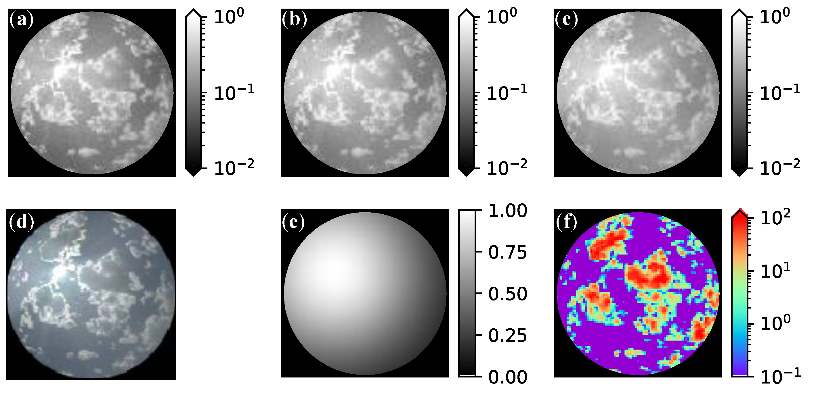
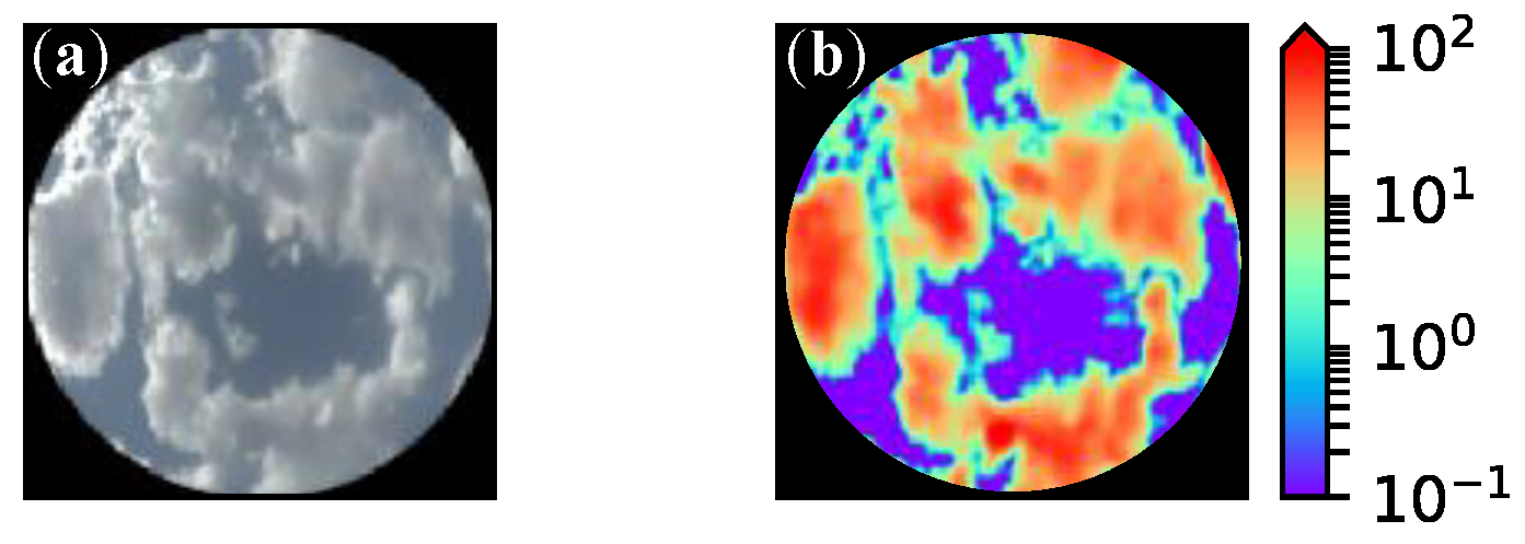
4.3. Examples of CNN Retrieval

The estimation accuracy of the trained CNN model was evaluated using the test data. Figure 10 shows examples of the ground truth and estimated SCOT. Figure 10a,b shows small broken clouds, Figure 11c shows a case of relatively homogeneous thin cloud, Figure 10d shows a case of large thin broken cloud, Figure 10e–h correspond to stratocumulus clouds with small gaps, and Figure 10i shows a very optically thick cloud. In all cases, SCOT seems to be reasonably estimated, and even small clouds are accurately detected. The CNN adequately reproduces the fact that the clouds are optically thick at the central part and become optically thin near the edges. The CNN can overcome the COT ambiguity by using the spatial features learned from the training data.
The complex non-linear relationship between COT and radiance caused by the 3D radiative effect is also learned by the CNN. A closer analysis of the results shows that the spatial distribution of the estimated COT on small scales. Large estimation errors exceeding 100% occur locally, suggesting that fine-scale fluctuations are difficult to reproduce using the present technique.

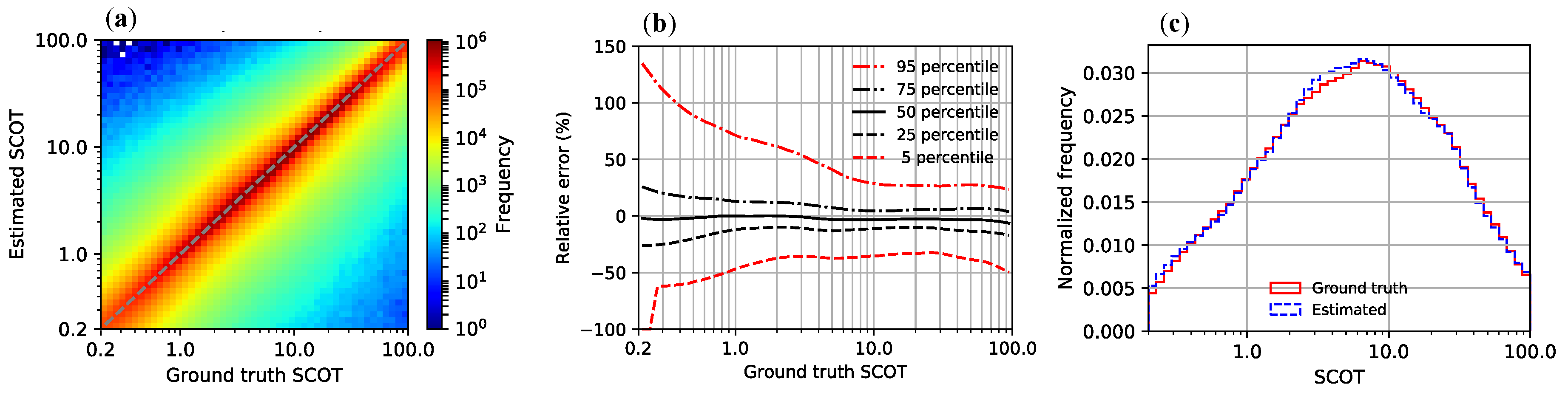
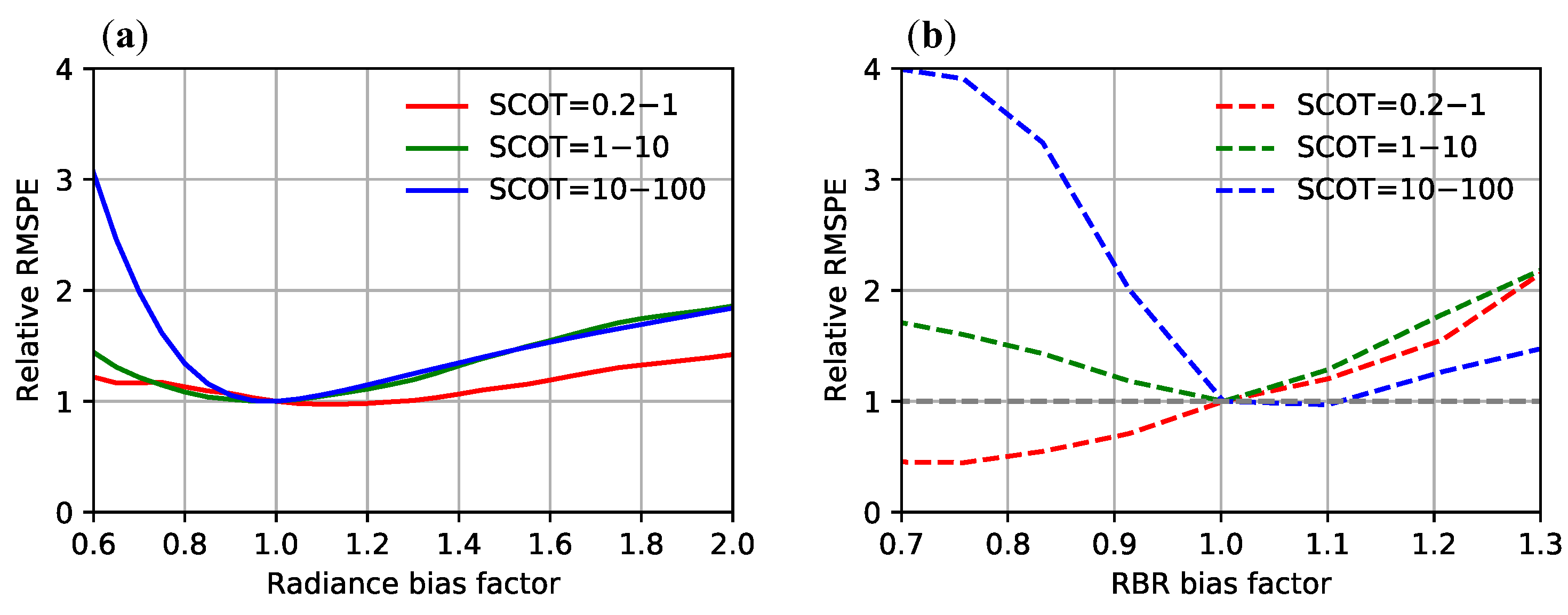
4.4. Evaluation of Retrieval Error

The statistical results of the SCOT retrieval error using all o the test data are shown in Figure 11. As can be seen in the joint histogram of the estimated and ground-truth SCOTs (Figure 11a), most of the data are concentrated near the diagonal line. There is a high correlation between the estimated and ground-truth SCOTs, with a correlation coefficient of 0.84. Figure 11b shows the relative error percentiles of the estimated SCOT as functions of the ground truth SCOT. The 50th percentile is between –7% and 1% for all of the SCOT ranges, and the 25th and 75th percentiles are within a range of ±15% for SCOT ≥1. For 0.2 ≤ SCOT ≤ 1, the variation in the relative error increases, but the 25th and 75th percentiles are still within ± 26%. When SCOT is close to 0.2, the 5th percentile is –100%, and the 95th percentile increases rapidly. The reason for the decrease in estimation accuracy for the very small SCOT is that the radiance sensitivity to COT is low (Figure 3a) and that the AOT and surface albedo are uncertain [47]. In this study, training data were generated assuming randomly chosen AOT and surface albedo values, and the CNN model assumes that the AOT and surface albedo are completely uncertain when estimating SCOT. It is remarkable that the CNN model can stably estimate SCOT with reasonable accuracy, even with an uncertain AOT and surface albedo. On the other hand, in the RRBR method [7], the increase of the observed (3D) radiance due to the illuminating effect leads to an underestimation of COT, and a large negative bias of over –50% has been reported when COT ≥30, which is consistent with the results in Figure 6. However, in our results, the bias is significantly reduced, which is because of the training based on the 3D radiative transfer model. The histogram of the estimated SCOT shows a very good agreement with the ground-truth histogram (Figure 11c), which suggests that the statistical distribution of SCOT can be adequately reproduced.
Table 2 summarizes the RMSPE, mean absolute percentage error (MAPE), and mean bias percentage error (MBPE) for different ranges of SCOT and cloud fraction. MAPE and MBPE are defined by the following equations:
MAPE = 1 n k = 1 n | ϵ k |
MBPE = 1 n k = 1 n ϵ k
Error evaluation was performed for pixels with VZA ≤43°. RMSPE is 87% when all the data are used for evaluation. RMSPE is reduced to 23% when the cloud fraction is ≥0.7, and SCOT is ≥ 1. Under broken clouds with a small cloud fraction, the 3D radiative transfer effects are large, which results in large estimation error. Additionally, RMSPE tends to be large when SCOT < 1. This is mainly caused by the uncertainty in AOT, as described above, which may cause extremely large relative errors in a small number of pixels when SCOT ≈ 0.2 (Figure 11a,b). MAPE is 1.5–5 times smaller than RMSPE. The MBPE ranges from –1.7% to 4.2% when the cloud amount is 0.7 or more, and ranges from –11.7% to 21.1% when the cloud amount is smaller than 0.7.
So far, it has been assumed that the radiometric calibration of the digital camera is accurate, that is, the RGB radiances are accurate. However, if the calibration is biased, the SCOT can be overestimated or underestimated. We examined how the bias in the radiometric calibration affects the estimation error of SCOT. The amplification factors of the RMSPE of the estimated SCOT with respect to a case of perfect calibration are shown in Figure 12. In Figure 12a, all of the RGB channels are equally biased, with a bias factor from 0.6 to 2.0. The RMSPE is indeed the smallest when there is no radiance bias, and the RMSPE increases by increasing the positive and negative bias. When the bias factor is in the range of 0.75–1.7, the RMSPE does not increase significantly, with an amplification factor of 1.5 or less.
In other words, the estimation of SCOT does not deteriorate if the error in absolute calibration of the camera is not excessive. On the other hand, Figure 12b shows the estimated error amplification of SCOT when the RBR is biased. When SCOT is 10 or more, and RBR has a negative bias (more bias in the blue channel than the red channel), the RMSPE of the SCOT rapidly increases. Thus, the SCOT estimation is relatively sensitive to the RBR bias. The RBR bias factor should be within 0.95–1.17 in order to keep the RMSPE amplification factor less than 1.5. Although the relative channel responses need to be calibrated with moderate accuracy, the SCOT retrieval is not very sensitive to the absolute calibration of radiance, which could be a reflection of the fact that the CNN model mainly uses the structural context for the SCOT retrieval.

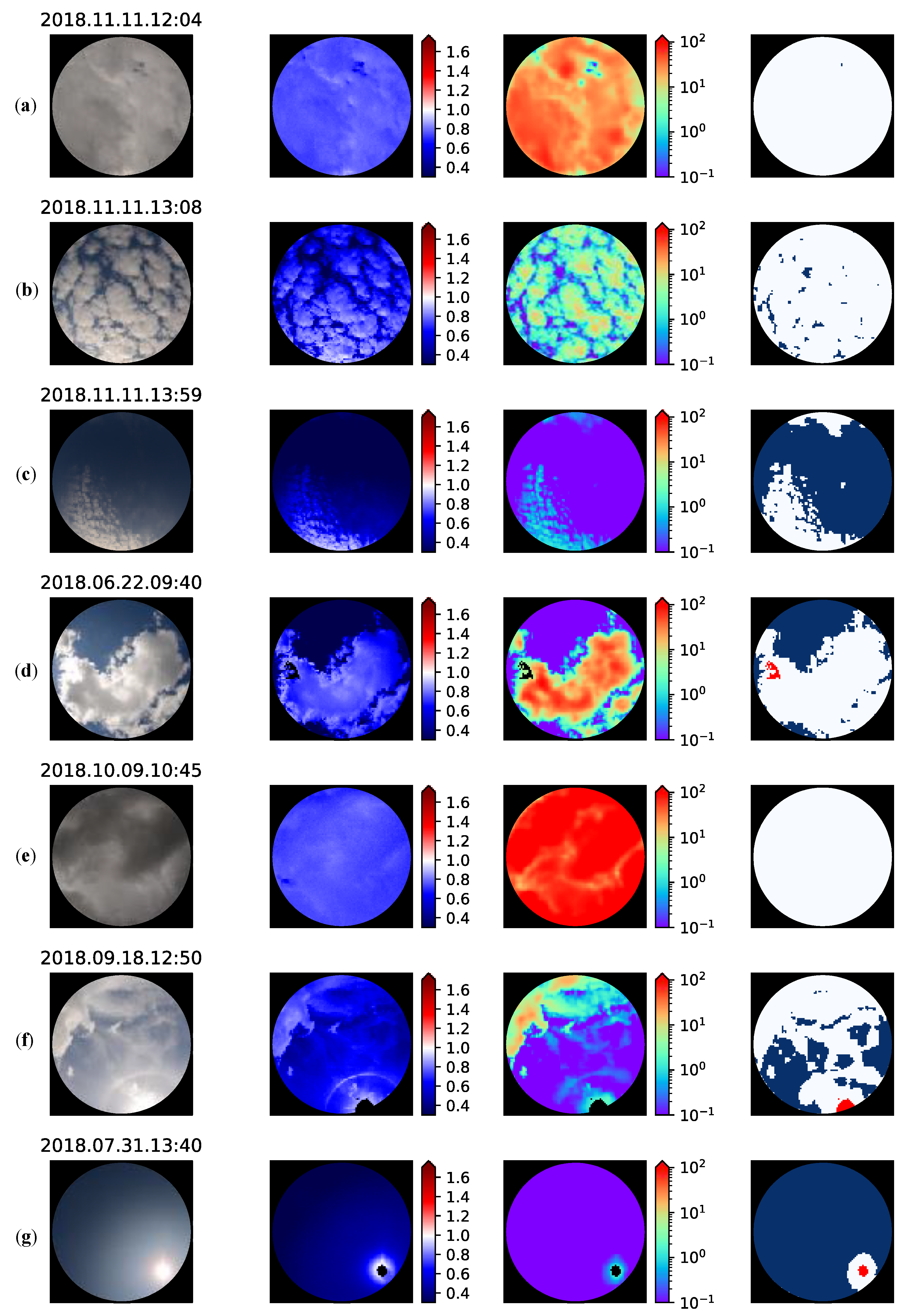
5. Applications to Sky-View Camera Observations

5.1. Overview of Observation

Observations were made using a digital camera for 28 days between 22 June and 12 November 2018. From June to October 2018, the observation site was at the rooftop of a building of the Graduate School of Science, Tohoku University (140.84°E, 38.25°N, 158 m above sea level), and in November 2018, the observation site was at the rooftop of a building in Chiba University (140.10°E, 35.62°N, 21 m ASL). The digital camera was a Nikon D7000 with an AF DX Fish-eye-Nikkor lens (10.5 mm f/2.8G ED) with a diagonal angle of 180°. The camera was oriented in the zenith direction, the aperture size was set at the maximum f-value of 2.8, and the exposure time was adjusted according to the overall brightness at the time of observation. A radiometric calibration was performed in advance using equipment at the Japan Aerospace Exploration Agency (JAXA) Tsukuba Space Center. The coefficients for conversion from the digital counts of RAW-format images to the channel-mean spectral radiances and spectral response functions of the RGB channels were determined, and a correction of the vignetting effect was applied [48]. The RAW images were converted to the equidistant projection, the radiance values were averaged to 128 × 128 pixels, and the pixel radiances for VZA >45° were set to 0, as for with the training data.

5.2. Example Results

Examples of the estimation result obtained by the CNN are shown in Figure 13. In this section, pixels with SCOT ≥0.2 were identified as cloudy. The cases in Figure 13a–d appear to be water clouds in the boundary layer. The SCOT distribution and the cloud pixel detection seem reasonable for both the overcast clouds (Figure 13a) and small broken clouds (Figure 13c). The cloud spatial structure at various horizontal scales was trained by the CNN, thus capturing that the COT is large at the center of the cloud and small at the edges. In the example in Figure 13b, the sun is located at a low position in the image, and in the camera image and RBR image, there is a tendency for the sun side of the cloud to be bright and the RBR to be high. This azimuthal dependence does not appear in the estimated SCOT distribution, suggesting that the 3D radiative effects are corrected. In Figure 13e, the sky is very dark, being covered completely by optically thick clouds, with a very large estimated SCOT of around 100. In Figure 13f, there is a cloud with moderate SCOT on the upper left side of the image. On the lower right side, a 22° halo is visible around the sun, which is likely caused by cirrus cloud composed of ice crystals. The halo feature results in an estimated SCOT of ~0.3, and the SCOT pattern clearly shows a halo shape. As the CNN in this study was trained assuming water clouds exclusively, the SCOT estimation may not be correct when the scattering phase function is largely different from that of water droplets. Figure 13g shows a misidentification of cloud around the sun. This could be caused by a lens flare. When the light from a strong light source, such as direct sunlight, is an incident on the camera, stray light from the reflections at the lens surfaces and the lens barrel leaks to darker pixels around the bright pixels. It is known that fisheye lenses are easily affected by lens flare, particularly when the aperture is large. In this study, the lens flare effect was not included when training the CNN, so that inconsistency is present between the training data and the actual observational data. The example in Figure 13g suggests that lens flare causes clear-sky pixels to be possibly erroneously identified as optically thin cloud. There are two methods to reduce such adverse effects, namely: (1) to shield the sun at the time of observation and (2) to train the CNN model by including the lens flare effect.

5.3. Comparison with Pyranometer Measurements

In November 2018, an intensive observation experiment called the “Chiba Campaign” was conducted at Chiba University in order to observe the atmosphere with various instruments [49]. Chiba University has a SKYNET site, and the data and site information are available on the web (http://atmos3.cr.chiba-u.jp/skynet/chiba/chiba.html). Building on previous efforts (e.g., [50] and the references therein), the effective hemispherical-mean COT was estimated from the total downward irradiance observed by a pyranometer on 11 November. A look-up table of irradiance was generated from radiative transfer model calculations, assuming a plane-parallel homogeneous cloud with a constant CDER, and the COT was estimated from a one-minute average of irradiance obtained with 10-second intervals. The COT was not estimated when the transmittance (defined as the ratio of the recorded irradiance to the corresponding value that is theoretically expected for the clear sky case [51]) is equal to or more than 0.8, as it is difficult to determine the COT in such a high-transmittance case, possibly because of the enhanced radiation by illuminated cloud sides. The directional SCOT of each image pixel was estimated by the CNN from a digital camera, and was converted to an equivalent COT using Equation (12). The camera measurements were made every minute. The data with the closest observation times were used to compare the two methods (with a time lag of less than 30 seconds). The pyranometer cannot distinguish between clear sky and cloudy regions within the hemispheric field of view. Therefore, it is reasonable to compare it with the COT averaged over the field of view of the digital camera with VZA ≤43°, including the clear-sky pixels with zero COT. For this day, the COT estimated from the downward irradiance resulted in being in relatively good agreement with the other estimates retrieved from both co-located instruments and satellites [49].
Figure 14 shows a comparison of the COT estimates from the pyranometer and camera. When the transmittance was high, the COT estimation was not actually performed using the pyranometer, but for convenience, the COT estimated from the pyranometer was set to 0 in this comparison. The temporal variations of COT obtained by the two methods are similar, with a correlation coefficient as high as 0.721. The COT obtained from the camera is overestimated, with mean bias of 0.702 compared to that from the pyranometer. The variability of COT obtained from the camera is also larger than that of the COT obtained from the pyranometer. A possible reason for this is that the pyranometer-based estimate is more spatiotemporally averaged in order to obtain smaller fluctuations than that obtained from the camera. Whereas the pyranometer has a field of view of a solid angle of 2π sr, the camera COT is averaged over a field of view of a solid angle of 0.586 × π sr (VZA ≤43°) centered on the zenith. Additionally, while the camera captures instantaneous values, one-minute average irradiance was used for obtaining COT from the pyranometer. For the camera, the COT of each pixel is first determined, and the spatial variations of the COT are then averaged. On the other hand, for the pyranometer, the variation of radiance within the field of view is averaged at the time of measurement. In general, COT has large spatial and temporal variations, and also has a strong nonlinearity with radiation. In heterogeneous cloud fields, averaging in the radiance space and averaging in the COT space may lead to different results.
At around 12:50 and 14:00, the COT obtained from the pyranometer is evidently larger than the COT obtained from the camera. As shown in the photograph in Figure 13c, at these times, the clouds cover a small fraction of the sky, and visually appear optically thin. If the instruments are under a cloud shadow, the pyranometer measures low global irradiance, as the direct sunlight is shadowed and the diffuse radiation from the above is weak because of the absence of significant scattering by clouds. This may cause a significant disagreement between the pyranometer and camera. The radiation enhancement can cause an opposite effect on the pyranometer; downward irradiance is enhanced and possibly exceeds a theoretical value for the clear sky case, resulting in the underestimation of COT obtained from the pyranometer. If cases are excluded when the COT obtained from either the pyranometer or camera is smaller than 1.5, the correlation coefficient becomes as high as 0.748. This kind of comparison is useful to characterize different algorithms and to identify possible 3D radiative effects, although a systematic study is needed in order to draw a conclusion. More detailed analyses including comparisons with different ground- and satellite-based instruments are presented in a separate paper [49].

6. Conclusions

A new method has been proposed for the estimation of the whole-sky spatial distribution of SCOT from images taken by a digital camera installed on the ground, by training a CNN based on a 3D radiative transfer model. Two CNNs were tested in this study. First, the effects of 3D radiative transfer on transmitted radiance, which was not well understood, has been investigated by model calculations. Under broken clouds, the 3D radiative effects, such as the radiation enhancement on the sun side of the cloud and cloud shadow on the opposite side, are significant. It was confirmed that the radiance is not determined by the local COT, but is strongly dependent on the spatial arrangement of the adjacent cloud elements. In order to estimate the local COT, it is essential to consider the spatial arrangement of the adjacent cloud elements. A comparison of different NN and CNN architectures experimentally confirmed that the multi-pixel method using multi-pixel data including surrounding pixels is effective. Subsequently, based on these findings, we have developed a deep CNN for SCOT retrieval from a sky-view camera. Evaluations using synthetic data showed that the CNN can accurately and rapidly estimate the spatial distribution of the SCOT from multi-channel camera images. For SCOTs in the range of 1–100, the bias and dispersion of the error were stable and small, with a significant reduction in the number of artifacts caused by 3D radiative effects, which had been a problem in previous research. The results show that the CNN reproduces the spatial feature of the cloud that the COT decreases from the center to the edges of the cloud, suggesting that the CNN is adequately trained to represent this spatial feature. Information about the spectral dependency of the radiance in the visible region is also used as supplementary information, and the spectral properties of the camera need to be accurately calibrated. On the other hand, the CNN estimation does not strongly depend on the absolute value of radiance, and is relatively robust against an uncertainty of about 20% of radiance calibration. However, when the SCOT is small, the uncertainty in the aerosol amount makes the estimation accuracy of SCOT low.
The CNN-based COT estimation has been applied to the images obtained by a digital camera that was radiometrically calibrated beforehand. The spatial distribution of the estimated COT did not show significant dependence on the solar direction, suggesting that the 3D radiative effects were effectively corrected. As an initial test, the camera retrieval was compared with the effective hemispherical-mean COT estimated from a pyranometer for one day, and a high correlation was shown. The COT estimated from the camera has a larger temporal variability, which may be caused by the differences in (1) the size of the field of view and (2) the time–space averaging method between the digital camera and the pyranometer.
The next steps are to analyze more diverse clouds, including ice clouds, so as to improve the accuracy and resolution of the training data, and to conduct more validation work by comparisons with independent observations. By increasing the resolution of the camera images used for estimation, it is possible to better capture small-scale spatial features of clouds [52]. This study is unique in that the spatial distribution of COT can be quickly estimated from a ground-based camera. This estimation can be useful as an initial guess in advanced cloud tomography [23,24,25,27], for the prediction and diagnosis of solar energy production, and for the validation of satellite cloud products.

Author Contributions

Conceptualization, H.I.; methodology, R.M. and H.I.; software, R.M. and H.I.; validation, R.M.; formal analysis, R.M. and A.D.; investigation, R.M.; resources, H.I.; data curation, R.M.; writing (original draft preparation), R.M.; writing (review and editing), H.I., K.S.S., A.D., and R.K.; visualization, R.M. and H.I.; supervision, H.I. and K.S.S.; project administration, H.I.; funding acquisition, H.I. and R.K.

Funding

This research was funded by a Grant-in-Aid for Scientific Research, grant number Kiban B 17H02963, from the Japan Society for the Promotion of Science (JSPS), and the Second Research Announcement on the Earth Observations of the Japan Aerospace Exploration Agency (JAXA), PI number ER2GCF204. A.D.’s work was funded by the JST CREST, grant number JPMJCR15K4.

Acknowledgments

SCALE-LES was developed by the SCALE interdisciplinary team at the RIKEN Advanced Institute for Computational Science (AICS), Japan. Parts of the results in this paper were obtained using the K supercomputer at RIKEN AICS. The authors are grateful to Dr. Yousuke Sato of Hokkaido University and Dr. Tomita of AICS, REKEN, for providing the SCALE-LES simulation data, and to Dr. Hitoshi Irie for organizing the Chiba campaign. The results of the radiative transfer simulations in this paper were obtained using the Reedbush supercomputer system of the University of Tokyo.

Conflicts of Interest

The authors declare no conflict of interest.

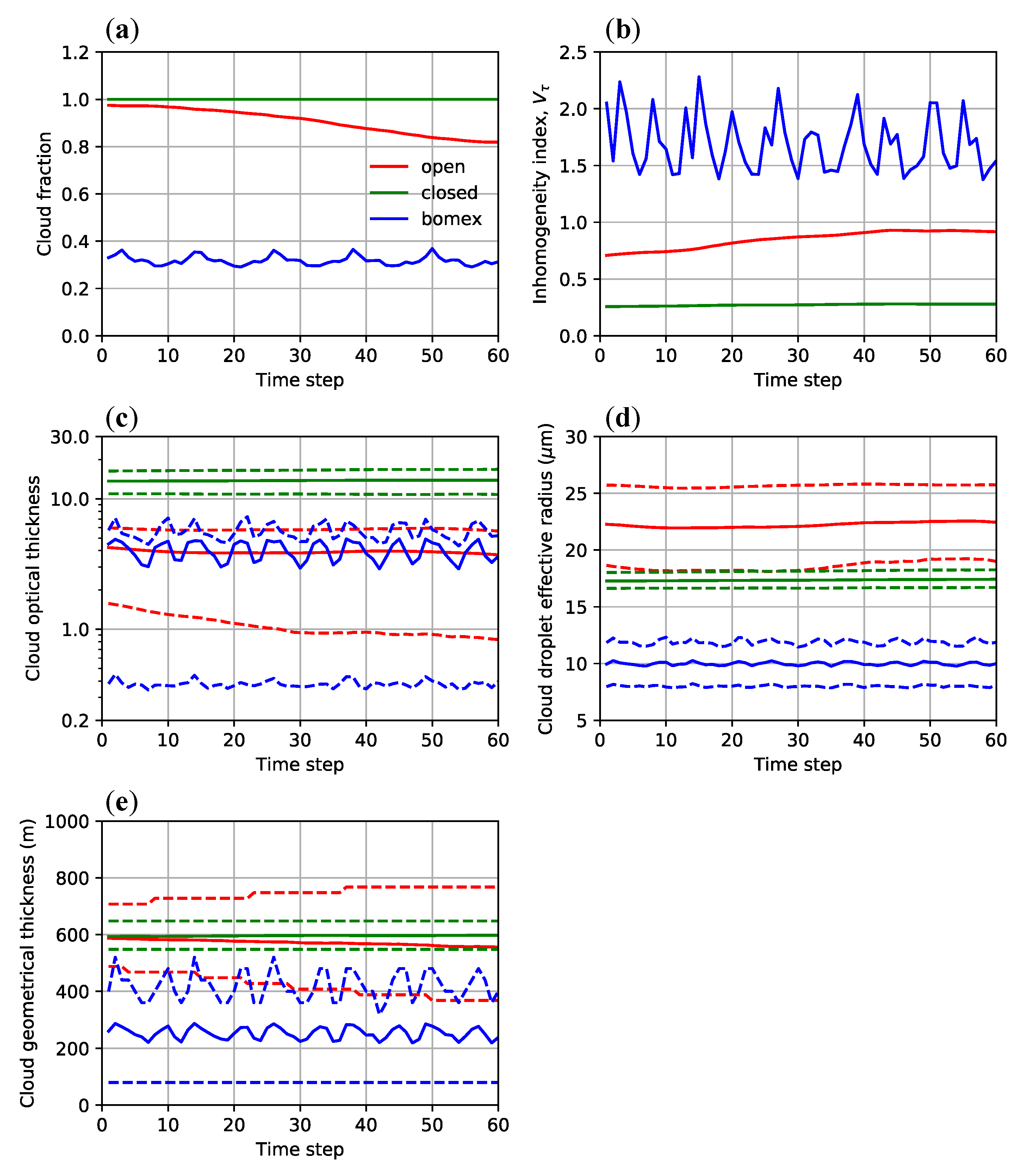
Appendix A. Clouds Simulated by SCALE-LES

Figure A1 shows the temporal variation of cloud in the three SCALE-LES simulation cases (open-cell, closed-cell, and BOMEX cases). The coefficient of variation of COT is defined as the horizontal heterogeneity index V τ , as follows:
V τ = σ τ τ ¯
where τ ¯ and σ τ represent the mean and standard deviation, respectively, of COT at 550 nm for the cloudy pixels. A large V τ indicates that clouds are horizontally heterogeneous. In the closed-cell case, the clouds maintain a nearly constant average COT over all of the time steps. In the open case, the cloud fraction decreases, and the clear sky spreads with advancing time steps. The horizontal heterogeneity is moderate. In the BOMEX case, the horizontal heterogeneity is larger than in the other two cases.
Figure A1. Temporal variations of cloud physical properties in the three cases simulated by the SCALE-LES model, namely: (a) cloud fraction; (b) the horizontal inhomogeneity index defined in Equation (5). (c,d,e) Domain average (solid lines) and 20th and 80th percentiles (dashed lines) of cloud optical thickness, column-mean droplet effective radius, and cloud geometrical thickness, respectively, calculated for the cloudy columns. All of the calculations are made by assuming that cloudy columns have a COT greater than or equal to 0.1.
Remotesensing 11 01962 g0a1

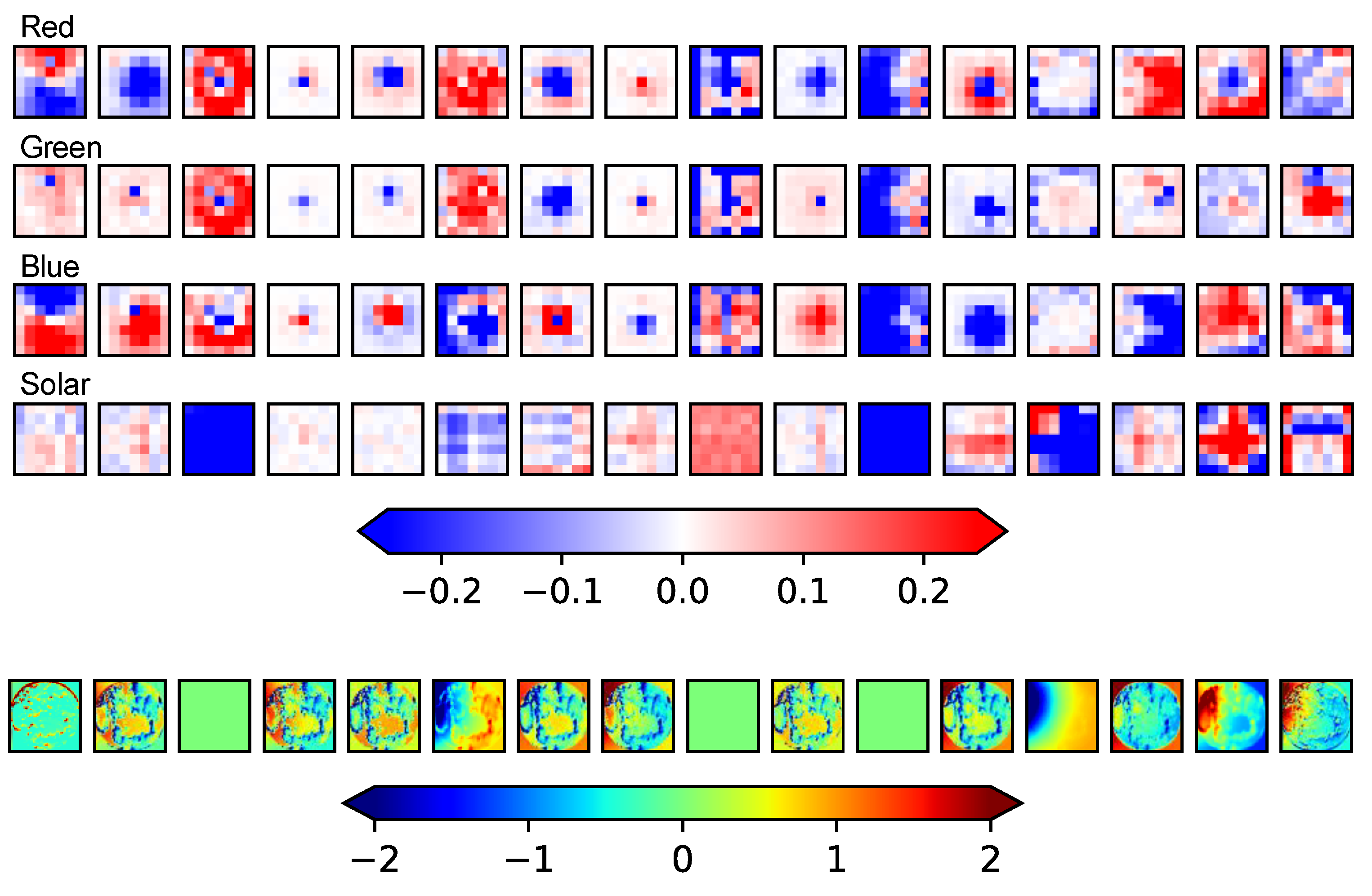
Appendix B. Anatomy of the CNN

In order to understand how the CNN extracts features from the input images, we show the convolution filters and the output feature maps from the middle layer of the CNN with the structure shown in Figure 9. We take the case of Figure A2 as an example, in which the sun is located outside of the image in the upper left direction, with solar zenith angle of 69.7°. Figure A3 shows the filters and output of the convolution layer (shown as A2 in Figure 9). These were trained so as to capture the features of the spatial distribution of radiance, depending on the spatial structure of the clouds and the positional relationship between the sun and the clouds. In the filters corresponding to the RGB channels, there are many patterns in which positive and negative signs appear at the center and periphery of the filter. Spatial patterns are isotropic or anisotropic. Additionally, there are many filters in which the red channel and blue channel have opposite signs, and these filters seem to capture the spectral features of radiance in the same way that RBR captures the spectral feature. Some portion of the output images clearly shows the edges of cloud, and other images show large values in the directions near the sun. Figure A4 shows the output feature maps of the convolutional layer of Figure 9 (A3). Various patterns have variations on different spatial scales. In some feature maps, the spatial pattern strongly depend on the position of the sun. Figure A5 shows half of the output feature maps of the convolutional layer of Figure 9 (A4), while the total number of output channels of (A4) is actually 512. There is a great variety of patterns, but it is currently difficult to interpret the meaning of the features in the deep layers. It is generally known to be more difficult to understand features of the deeper layers in deep NN.
Figure A2. Examples of (a) an input true-color image and (b) estimated SCOT. The sun is located outside of the image in the upper left direction, with solar zenith and azimuth angles of 69.7° and 195.5°, respectively. In this image, the azimuth is defined to be positive in the clockwise direction from the right.
Remotesensing 11 01962 g0a2
Figure A3. Upper panels show the multi-channel filters in the first convolution layer (A2) shown in Figure 9. Each column corresponds to one of 16 filters, and each row corresponds to one of four input channels. The filter size is 7 × 7 pixels, and the color shades represent the filter weight. The lower panels show output feature maps with a size of 128 × 128 pixels for the case shown in Figure A2, where each image corresponds to the above multi-channel convolution filters. Each feature map shows normalized signals with a mean of 0 and standard deviation of 1, except for the third, ninth, and eleventh ones from the left, for which the standard deviation is less than 10−35.
Remotesensing 11 01962 g0a3
Figure A4. Feature maps with a size of 32 × 32 pixels that are output from the last convolution layer of the residual block (A3) shown in Figure 9, for the case shown in Figure A2. All 64 feature maps are shown. Each image shows the normalized signal of the feature map with a mean of 0 and standard deviation of 1.
Remotesensing 11 01962 g0a4
Figure A5. Selected feature maps with a size of 16 × 16 pixels that are output from the convolution layer (A4) shown in Figure 9, for the case shown in Figure A2. Half (256) of the 512 feature maps are arbitrarily shown. Each image shows the normalized signal of the feature map with a mean of 0 and standard deviation of 1.
Remotesensing 11 01962 g0a5

References

  1. Chow, C.W.; Urquhart, B.; Lave, M.; Dominguez, A.; Kleissl, J.; Shields, J.; Washom, B. Intra-hour forecasting with a total sky imager at the UC San Diego solar energy testbed. Sol. Energy 2011, 85, 2881–2893. [Google Scholar] [CrossRef] [Green Version]
  2. Marshak, A.; Knyazikhin, Y.; Evans, K.D.; Wiscombe, W.J. The “RED versus NIR” plane to retrieve broken-cloud optical depth from ground-based measurements. J. Atmos. Sci. 2004, 61, 1911–1925. [Google Scholar] [CrossRef]
  3. Chiu, J.C.; Huang, C.-H.; Marshak, A.; Slutsker, I.; Giles, D.M.; Holben, B.N.; Knyazikhin, Y.; Wiscombe, W.J. Cloud optical depth retrievals from the Aerosol Robotic Network (AERONET) cloud mode observations. J. Geophys. Res. 2010, 115, 14202. [Google Scholar] [CrossRef]
  4. Kikuchi, N.; Nakajima, T.; Kumagai, H.; Kuroiwa, H.; Kamei, A.; Nakamura, R.; Nakajima, T.Y. Cloud optical thickness and effective particle radius derived from transmitted solar radiation measurements: Comparison with cloud radar observations. J. Geophys. Res.-Atmos. 2006, 111, 07205. [Google Scholar] [CrossRef]
  5. McBride, P.J.; Schmidt, K.S.; Pilewskie, P.; Kittelman, A.S.; Wolfe, D.E. A spectral method for retrieving cloud optical thickness and effective radius from surface-based transmittance measurements. Atmos. Chem. Phys. 2011, 11, 7235–7252. [Google Scholar] [CrossRef] [Green Version]
  6. Niple, E.R.; Scott, H.E.; Conant, J.A.; Jones, S.H.; Iannarilli, F.J.; Pereira, W.E. Application of oxygen A-band equivalent width to disambiguate downwelling radiances for cloud optical depth measurement. Atmos. Meas. Tech. 2016, 9, 4167–4179. [Google Scholar] [CrossRef] [Green Version]
  7. Mejia, F.A.; Kurtz, B.; Murray, K.; Hinkelman, L.M.; Sengupta, M.; Xie, Y.; Kleissl, J. Coupling sky images with radiative transfer models: A new method to estimate cloud optical depth. Atmos. Meas. Tech. 2016, 9, 4151–4165. [Google Scholar] [CrossRef]
  8. Cahalan, R.F.; Ridgway, W.; Wiscombe, W.J.; Bell, T.L.; Snider, J.B. The albedo of fractal stratocumulus clouds. J. Atmos. Sci. 1994, 51, 2434–2455. [Google Scholar] [CrossRef]
  9. Loeb, N.G.; Várnai, T.; Davies, R. Effect of cloud inhomogeneities on the solar zenith angle dependence of nadir reflectance. J. Geophys. Res. Atmos. 1997, 102, 9387–9395. [Google Scholar] [CrossRef]
  10. Várnai, T.; Davies, R. Effects of cloud heterogeneities on shortwave radiation: Comparison of cloud-top variability and internal heterogeneity. J. Atmos. Sci. 1999, 56, 4206–4224. [Google Scholar] [CrossRef]
  11. Várnai, T.; Marshak, A. Observations of three-dimensional radiative effects that influence MODIS cloud optical thickness retrievals. J. Atmos. Sci. 2002, 59, 1607–1618. [Google Scholar] [CrossRef]
  12. Kato, S.; Hinkelman, L.M.; Cheng, A. Estimate of satellite-derived cloud optical thickness and effective radius errors and their effect on computed domain-averaged irradiances. J. Geophys. Res. Atmos. 2006, 111, 17201. [Google Scholar] [CrossRef]
  13. Marshak, A.; Platnick, S.; Várnai, T.; Wen, G.; Cahalan, R.F. Impact of three-dimensional radiative effects on satellite retrievals of cloud droplet sizes. J. Geophys. Res. Atmos. 2006, 111, 09207. [Google Scholar] [CrossRef]
  14. Iwabuchi, H.; Hayasaka, T. A multi-spectral non-local method for retrieval of boundary layer cloud properties from optical remote sensing data. Remote Sens. Environ. 2003, 88, 294–308. [Google Scholar] [CrossRef]
  15. Faure, T.; Isaka, H.; Guillemet, B. Neural network retrieval of cloud parameters of inhomogeneous and fractional clouds: Feasibility study. Remote Sens. Environ. 2001, 77, 123–138. [Google Scholar] [CrossRef]
  16. Faure, T.; Isaka, H.; Guillemet, B. Neural network retrieval of cloud parameters from high-resolution multispectral radiometric data: A feasibility study. Remote Sens. Environ. 2002, 80, 285–296. [Google Scholar] [CrossRef]
  17. Cornet, C.; Isaka, H.; Guillemet, B.; Szczap, F. Neural network retrieval of cloud parameters of inhomogeneous clouds from multispectral and multiscale radiance data: Feasibility study. J. Geophys. Res. Atmos. 2004, 109, 12203. [Google Scholar] [CrossRef]
  18. Cornet, C.; Buriez, J.C.; Riédi, J.; Isaka, H.; Guillemet, B. Case study of inhomogeneous cloud parameter retrieval from MODIS data. Geophys. Res. Lett. 2005, 32, 13807. [Google Scholar] [CrossRef]
  19. Evans, K.F.; Marshak, A.; Várnai, T. The potential for improved boundary layer cloud optical depth retrievals from the multiple directions of MISR. J. Atmos. Sci. 2008, 65, 3179–3196. [Google Scholar] [CrossRef]
  20. Okamura, R.; Iwabuchi, H.; Schmidt, S. Feasibility study of multi-pixel retrieval of optical thickness and droplet effective radius of inhomogeneous clouds using deep learning. Atmos. Meas. Tech. 2017, 10, 4747–4759. [Google Scholar] [CrossRef] [Green Version]
  21. Marín, M.J.; Serrano, D.; Utrillas, M.P.; Núñez, M.; Martínez-Lozano, J.A. Effective cloud optical depth and enhancement effects for broken liquid water clouds in Valencia (Spain). Atmos. Res. 2017, 195, 1–8. [Google Scholar] [CrossRef]
  22. Fielding, M.D.; Chiu, J.C.; Hogan, R.J.; Feingold, G. A novel ensemble method for retrieving properties of warm cloud in 3-D using ground-based scanning radar and zenith radiances. J. Geophys. Res. Atmos. 2014, 119, 10912–10930. [Google Scholar] [CrossRef]
  23. Levis, A.; Schechner, Y.; Aides, A. Airborne Three-Dimensional Cloud Tomography. In Proceedings of the IEEE International Conference on Computer Vision, Santiago, Chile, 7–13 December 2015; pp. 3379–3387. [Google Scholar] [CrossRef]
  24. Levis, A.; Schechner, Y.Y.; Davis, A.B. Multiple-scattering Microphysics Tomography. In Proceedings of the IEEE Conference on Computer Vision and Pattern Recognition (CVPR), Honolulu, HI, USA, 21–26 July 2017; pp. 6740–6749. [Google Scholar]
  25. Holodovsky, V.; Schechner, Y.Y.; Levin, A.; Levis, A.; Aides, A. In-situ Multi-view Multi-scattering Stochastic Tomography. In Proceedings of the 2016 IEEE International Conference on Computational Photography (ICCP), Evanston, IL, USA, 13–15 May 2016; pp. 1–12. [Google Scholar] [CrossRef]
  26. Martin, W.G.K.; Hasekamp, O.P. A demonstration of adjoint methods for multi-dimensional remote sensing of the atmosphere and surface. J. Quant. Spectrosc. Radiat. Transf. 2018, 204, 215–231. [Google Scholar] [CrossRef]
  27. Mejia, F.A.; Kurtz, B.; Levis, A.; de la Parra, I.; Kleissl, J. Cloud tomography applied to sky images: A virtual testbed. Sol. Energy 2018, 176, 287–300. [Google Scholar] [CrossRef]
  28. Sato, Y.; Nishizawa, S.; Yashiro, H.; Miyamoto, Y.; Tomita, H. Potential of retrieving shallow-cloud life cycle from future generation satellite observations through cloud evolution diagrams: A suggestion from a large eddy simulation. Sci. Online Lett. Atmos. 2014, 10, 10–14. [Google Scholar] [CrossRef]
  29. Sato, Y.; Nishizawa, S.; Yashiro, H.; Miyamoto, Y.; Kajikawa, Y.; Tomita, H. Impacts of cloud microphysics on trade wind cumulus: Which cloud microphysics processes contribute to the diversity in a large eddy simulation? Prog. Earth Planet. Sci. 2015, 2, 23. [Google Scholar] [CrossRef]
  30. Nishizawa, S.; Yashiro, H.; Sato, Y.; Miyamoto, Y.; Tomita, H. Influence of grid aspect ratio on planetary boundary layer turbulence in large-eddy simulations. Geosci. Model Dev. 2015, 8, 3393–3419. [Google Scholar] [CrossRef] [Green Version]
  31. Iwabuchi, H. Efficient Monte Carlo methods for radiative transfer modeling. J. Atmos. Sci. 2006, 63, 2324–2339. [Google Scholar] [CrossRef]
  32. Iwabuchi, H.; Okamura, R. Multispectral Monte Carlo radiative transfer simulation by the maximum cross-section method. J. Quant. Spectrosc. Radiat. Transf. 2017, 193, 40–46. [Google Scholar] [CrossRef]
  33. Hänel, G. The properties of atmospheric aerosol particles as functions of the relative humidity at thermodynamic equilibrium with the surrounding moist air. Adv. Geophys. 1976, 19, 73–188. [Google Scholar]
  34. Zhao, H.; Shi, J.; Qi, X.; Wang, X.; Jia, J. Pyramid Scene Parsing Network. In Proceedings of the IEEE Conference on Computer Vision and Pattern Recognition (CVPR), Honolulu, HI, USA, 21–26 July 2017; pp. 2881–2890. [Google Scholar]
  35. He, K.; Zhang, X.; Ren, S.; Sun, J. Deep Residual Learning for Image Recognition. In Proceedings of the IEEE Conference on Computer Vision and Pattern Recognition, Las Vegas, NV, USA, 27–30 June 2016; pp. 770–778. [Google Scholar]
  36. He, K.; Zhang, X.; Ren, S.; Sun, J. Identity Mappings in Deep Residual Networks. In European Conference on Computer Vision; Springer: Cham, Switzerland, 2016; pp. 630–645. [Google Scholar] [Green Version]
  37. Zagoruyko, S.; Komodakis, N. Wide Residual Networks. In Proceedings of the British Machine Vision Conference (BMVC), York, UK, 19–22 September 2016; BMVA Press: Durham, UK, 2016; pp. 87.1–87.12. [Google Scholar]
  38. Ioffe, S.; Szegedy, C. Batch Normalization Accelerating Deep Network Training by Reducing Internal Covariate Shift. In Proceedings of the 32nd International Conference on Machine Learning, Lille, France, 7–9 July 2015; p. 37. [Google Scholar]
  39. Goodfellow, I.J.; Bengio, Y.; Courville, A. Deep Learning; MIT Press: Cambridge, MA, USA, 2016. [Google Scholar]
  40. Kingma, D.P.; Ba, J. Adam: A Method for Stochastic Optimization CoRR, abs/1412.6980. In Proceedings of the 3rd International Conference on Learning Representations (ICLR 2015), San Diego, CA, USA, 7–9 May 2015. [Google Scholar]
  41. Tokui, S.; Oono, K.; Hido, S.; Clayton, J. Chainer: A Next-generation Open Source Framework for Deep Learning. In Proceedings of the Workshop on Machine Learning Systems (LearningSys) in the Twenty-Ninth Annual Conference on Neural Information Processing Systems (NIPS), Montreal CANADA , 7–12 December 2015; Volume 5, pp. 1–6. [Google Scholar]
  42. Marshak, A.; Davis, A. 3D Radiative Transfer in Cloudy Atmospheres; Springer Science Business Media: Berlin, Heidelberg, Germany; New York, NY, USA, 2005. [Google Scholar]
  43. Chen, L.C.; Papandreou, G.; Kokkinos, I.; Murphy, K.; Yuille, A.L. Semantic Image Segmentation with Deep Convolutional Nets and Fully Connected CRFs. In Proceedings of the International Conference Learning Representations, San Diego, CA, USA, 7–9 May 2015. [Google Scholar]
  44. Yu, F.; Koltun, V. Multi-scale Context Aggregation by Dilated convolutions. In Proceedings of the International Conference Learning Representations, San Juan, PR, USA, 2–4 May 2016. [Google Scholar]
  45. Yu, F.; Koltun, V.; Funkhouser, T. Dilated residual networks. In Proceedings of the IEEE Conference on Computer Vision and Pattern Recognition, Honolulu, HI, USA, 21–26 July 2017; pp. 472–480. [Google Scholar]
  46. Loshchilov, I.; Hutter, F. Fixing weight decay regularization in Adam, CoRR, abs/1711.05101. In Proceedings of the ICLR 2018 Conference Blind Submission, Vancouver, BC, Canada, 30 April–3 May 2018. [Google Scholar]
  47. Zinner, T.; Hausmann, P.; Ewald, F.; Bugliaro, L.; Emde, C.; Mayer, B. Ground-based imaging remote sensing of ice clouds: Uncertainties caused by sensor, method and atmosphere. Atmos. Meas. Tech. 2016, 9, 4615–4632. [Google Scholar] [CrossRef]
  48. Saito, M.; Iwabuchi, H.; Murata, I. Estimation of spectral distribution of sky radiance using a commercial digital camera. Appl. Opt. 2016, 55, 415–424. [Google Scholar] [CrossRef]
  49. Damiani, A.; Irie, H.; Takamura, T.; Kudo, R.; Khatri, P.; Iwabuchi, H.; Masuda, R.; Nagao, T. An intensive campaign-based intercomparison of cloud optical depth from ground and satellite instruments under overcast conditions. Sci. Online Lett. Atmos. 2019, 15, 190–193. [Google Scholar] [CrossRef]
  50. Serrano, D.; Nunez, M.; Utrillas, M.P.; Marın, M.J.; Marcos, C.; Martınez-Lozano, J.A. Effective cloud optical depth for overcast conditions determined with a UV radiometers. Int. J. Climatol. 2014, 34, 3939–3952. [Google Scholar] [CrossRef]
  51. Damiani, A.; Irie, H.; Horio, T.; Takamura, T.; Khatri, P.; Takenaka, H.; Nagao, T.; Nakajima, T.Y.; Cordero, R. Evaluation of Himawari-8 surface downwelling solar radiation by ground-based measurements. Atmos. Meas. Tech. 2018, 11, 2501–2521. [Google Scholar] [CrossRef] [Green Version]
  52. Schwartz, S.E.; Huang, D.; Vladutescu, D.V. High-resolution photography of clouds from the surface: Retrieval of optical depth of thin clouds down to centimeter scales. J. Geophys. Res. Atmos. 2017, 122, 2898–2928. [Google Scholar] [CrossRef]
Figure 1. Examples of Scalable Computing for Advanced Library and Environment-Large Eddy Simulation (SCALE-LES) cumulus cloud fields for the following three cases: (a,b) closed-cell, (c,d) open-cell, and (e,f) Barbados Oceanographic and Meteorological Experiment (BOMEX). (a,c,e) Horizontal distribution of the cloud optical thickness (COT). (b,d,f) Vertical cross section of the volume extinction coefficient along the black dashed lines superimposed on (a,c,e), respectively. White lines in (b) indicate lines of sight from a ground-based camera.
Remotesensing 11 01962 g001
Figure 2. Examples of the spatial distributions of the zenith-viewing transmitted radiances at the ground, as follows: (a) true-color image composed of mean spectral radiances in the red, green, and blue (RGB) channels in the standard RGB (sRGB) color space defined by International Electrotechnical Commission, computed by three-dimensional (3D) radiative transfer; (b) the same as (a), but for radiances computed using the independent pixel approximation (IPA); (c) differences in the mean spectral radiance in the red channel between the 3D and IPA calculations; (d,e) red-to-blue ratio (RBR) of 3D and IPA, respectively; (f) COT. The sun is located in the left of the images, with a solar zenith angle of 60°. The regions framed by red squares correspond to the examples of image patches analyzed in detail in this study, and the regions framed by green squares correspond to pixels of the input and output for the convolutional neural network (CNN).
Remotesensing 11 01962 g002
Figure 3. (a) Spectral radiances of red and blue channels and (b) RBR, computed using the IPA and 3D radiative transfer as functions of COT, for the case in Figure 2. For the 3D results, solid lines and shaded areas denote the mean and standard deviation, respectively, of the values computed for each COT bin, where 30 bins are spaced equally on a logarithmic scale.
Remotesensing 11 01962 g003
Figure 4. Structure of a simplified version of a convolutional neural network (CNN) used for a test of COT estimation based on the zenith-viewing transmitted radiances. The input and output layers (yellow) are presented with the image size (in pixels) and the number of channels/variables. The input takes a multispectral image with three spectral channels, and the output is a two-dimensional distribution of COT. The neural network (NN) layers denoted in light blue and purple represent the convolutional and deconvolutional layers, respectively, shown with a filter size and the number of output channels. The “×1/2” represents the convolution to halve the size of the feature map. The NN layers denoted in pink represent the average pooling to obtain a feature map with a shown number of pixels. In the “upsample” layer, bilinear interpolation is performed to expand the feature map, in order to obtain the shown number of pixels. The “concat” layer concatenates all of the channels in the layer input. The layer blocks denoted by black dashed lines with marks (# and *) are the residual blocks with detailed structures, shown separately in the upper right. These consist of batch normalization (“batch norm”); a rectified linear (ReLU) activation function; and convolution with a 3 × 3 filter, dropout, and summation (“sum”) operators. More details are explained in the main text.
Remotesensing 11 01962 g004
Figure 5. Examples of COT retrieval by various methods, namely: (a) ground-truth COT, (bf) estimated COT, and (gk) relative errors in the estimated COT. (b,g) The radiance red-to-blue ratio (RRBR) method of Mejia et al. (2016), (c,h) NN-0-IPA, (d,i) NN-0-3D, (e,j) NN-M10-3D, and (f,k) CNN-3D. The details of each NN/CNN-based estimation model are summarized in Table 1. This sample has a size of 32 × 32 pixels, and corresponds to the region marked by a red square in Figure 2. The direct solar beam is incident from the left, with a solar zenith angle of 60°.
Remotesensing 11 01962 g005
Figure 6. Comparison of relative errors in the estimated COT obtained by various methods summarized in Table 1, namely: (a) RRBR method; (b) NN-0 method; (c) NN-1 method; (d) NN-3 method; (e) NN-10 method; (f) CNN. The solid lines denote the median values and the shaded areas denote ranges between the 25th and 75th percentiles. The NN models were trained using IPA and 3D radiances, respectively, and the estimation errors for the IPA- and 3D-based NN models were evaluated for the 3D radiances as the input.
Remotesensing 11 01962 g006
Figure 7. Root-mean-square percentage errors (RMSPEs) as functions of the number of input-image pixels of the multi-pixel NN (NN-M) estimation model for (a) COT = 0.2–1, (b) COT = 1–10, and (c) COT = 10–100. For the number M in the horizontal axis, the number of input-image pixels is (2M + 1)2, including the target pixel and surrounding pixels. For comparison, the RMSPE for the CNN-3D model is plotted with identical values, independent of the number of surrounding pixels.
Remotesensing 11 01962 g007
Figure 8. Example of the input and output of the CNN for the estimation of slant-column COT (SCOT) from the sky-camera images. Shown are the spectral radiances from the (a) red, (b) green, and (c) blue channels, normalized by dividing by 800 W m−2 sr−1 µm−1, (d) a true-color image, (e) a solar position image, and (f) the SCOT along the line of sight corresponding to each pixel. The spectral responses of a commercial digital camera with a fish-eye lens are predetermined and assumed in the simulations. The input to the CNN is a four-channel image composed of (ac,e), and the output is a single-channel image of (f). The solar zenith and azimuth angles are 26° and 184.2°, respectively. The centers of the images are oriented to the zenith, the field of view is within 45° from the center, and an equidistant projection is assumed.
Remotesensing 11 01962 g008
Figure 9. Structure of the CNN proposed in the present study for the estimation of slant-column COT (SCOT) from sky camera images. The input is three spectral channels with an additional solar position image. Layers denoted in light green represent the dilated convolutional layers with the shown filter size, number of output channels, and dilation parameter. The filters and an example of the feature maps of the layers denoted by (A2), (A3), and (A4) are presented in Figure A2, Figure A3, Figure A4 and Figure A5. The other notations are the same as in Figure 4. More details are explained in the text.
Remotesensing 11 01962 g009
Figure 10. Examples of SCOT estimated by the CNN for cases (a–i) in the test dataset. The leftmost column shows the true-color images, the two middle columns show the (left) ground-truth and (right) estimated SCOT, and the rightmost column shows the relative error (%) of the estimated SCOT.
Remotesensing 11 01962 g010
Figure 11. Evaluation of SCOT estimation by the CNN for the test dataset: (a) joint histogram of the estimated and ground-truth SCOT, with an occurrence frequency denoted by color shades; (b) relative error of the estimated SCOT as a function of the ground-truth SCOT; (c) comparison of histograms of the estimated and ground-truth SCOT.
Remotesensing 11 01962 g011
Figure 12. Sensitivities of the SCOT estimation error to (a) radiance bias and (b) RBR bias. The vertical axis is the RMSPE relative to the RMSPE, without radiance and RBR bias. For (a), the radiance bias with the same factor was assumed for all of the RGB channels. For (b), the biases of the red and blue channels are assumed to have opposite signs. A total of 100 samples from the test dataset were used to evaluate each case of biased input.
Remotesensing 11 01962 g012
Figure 13. Examples of SCOT estimated from a ground-based zenith-oriented digital camera. Cases (ag) correspond to single snapshots made at respective times shown in the title of the leftmost panel. The observation time is shown in the YYYY.MM.DD.HH:XX format, where YYYY denotes the year, MM the month, DD the day, HH the hour, and XX the minute. The columns from left to right show the camera images in JPEG format, the RBR, the estimated SCOT, and the cloud flag, respectively. The cloud flag is displayed with a white color for cloudy pixels, a navy-blue color for clear-sky pixels, and a red color for the pixels that are undetermined because of the saturation of the camera-image signals. The saturated pixels are indicated by black in the RBR and estimated SCOT images.
Remotesensing 11 01962 g013
Figure 14. Comparison of the average COT estimated from a zenith-oriented digital camera using the CNN, and the COT estimated using a pyranometer, for 11 November 2018, as follows: (a) time series with a one-minute interval; (b) a scatter plot of the COT estimated by the two methods. For the camera-based estimation, the COT values were converted from the SCOT obtained for every pixel, and averaged over a field within 43° from the center of the image. In (a), the three red dashed lines correspond to the times of Figure 13a,b,c, respectively. In (b), the correlation coefficient (r) is shown.
Remotesensing 11 01962 g014
Table 1. Tested neural network (NN) architectures for the estimation of cloud optical thickness (COT) from zenith-viewing transmitted radiance. Single-pixel (NN-0) and multi-pixel (NN-M for M = 1–10) architectures derive a single-pixel COT of the central pixel from single-pixel and multiple pixels’ radiance data. CNN denotes convolutional NN, which derives the multi-pixel COT from multiple pixels’ radiance data. The input image corresponds to the surrounding pixels used to derive COT at either the single central pixel in NN-M, or the whole image at once in CNN.
ModelArchitecture (Nodes)Input Image Size (Pixels)Output Image Size (Pixels)Number of Model Parameters (Millions)Number of EpochsTraining Time (h)
NN-0NN (64)110.0003215003.0
NN-1NN (288)3 × 310.008355003.0
NN-2NN (800)5 × 510.06165003.0
NN-3NN (1568)7 × 710.2345003.0
NN-4NN (2592)9 × 910.6355003.0
NN-5NN (3872)11 × 1111.415003.1
NN-6NN (5408)13 × 1312.755003.1
NN-7NN (7200)15 × 1514.875003.1
NN-8NN (9248)17 × 1718.045003.1
NN-9NN (11552)19 × 19112.55003.7
NN-10NN (14112)21 × 21118.75005.1
CNNPSPNet52 × 5252 × 5210.820000.35
Table 2. Summary of errors in estimated slant-column COT (SCOT) along the line of sight from the simulated sky-view camera image, evaluated for the test data set. The results are summarized for different cloud fraction and SCOT ranges.
Cloud FractionSCOT rangeRMSPE 1 (%)MAPE 1 (%)MBPE 1 (%)
0.71–1002313–0.2
0.2–10030140.3
0.2–169224.2
1–1026141.1
10–1001711–1.7
< 0.71–100118497.0
0.2–1001895212.6
0.2–12625621.1
1–101284812.9
10–1007750–11.7
all1–10048180.8
0.2–10087212.6
0.2–11913912.5
1–1059203.2
10–1002714–2.5
1 RMSPE, MAPE, and MBPE denote root-mean-square, mean absolute, and mean bias percentage errors, respectively.

