Oceanic Mesoscale Eddy Detection Method Based on Deep Learning

Abstract

Oceanic mesoscale eddies greatly influence energy and matter transport and acoustic propagation. However, the traditional detection method for oceanic mesoscale eddies relies too much on the threshold value and has significant subjectivity. The existing machine learning methods are not mature or purposeful enough, as their train set lacks authority. In view of the above problems, this paper constructs a mesoscale eddy automatic identification and positioning network—OEDNet—based on an object detection network. Firstly, 2D image processing technology is used to enhance the data of a small number of accurate eddy samples annotated by marine experts to generate the train set. Then, the object detection model with a deep residual network, and a feature pyramid network as the main structure, is designed and optimized for small samples and complex regions in the mesoscale eddies of the ocean. Experimental results show that the model achieves better recognition compared to the traditional detection method and exhibits a good generalization ability in different sea areas.

1. Introduction

Mesoscale eddies are a common and complex seawater flow phenomenon in the ocean. Due to their vertical structure and strong kinetic energy, mesoscale eddies play an important role in the mixing and transport of heat, salt, and biological and chemical tracers [1,2,3,4,5]. They have also been shown to affect near-surface winds, clouds, rainfall [6], hydroacoustic transmission, and marine ecosystems in nearby areas [7,8]. Therefore, the detection and characterization of mesoscale eddies is of great research value in the fields of marine meteorology, marine acoustics, and marine biology. However, due to the lack of an accurate definition of eddies themselves, there are still some problems in the detection algorithm proposed by scholars based on mesoscale eddy characteristics. At present, the most accurate method of oceanic mesoscale eddies relies on “expert visual interpretation” [9], which is time-consuming and laborious. In recent years, with the development of artificial intelligence and the continuous upgrading of computer hardware, researchers have tried to establish a neural network via deep learning that simulates the human brain for analysis and learning, extracting higher-level and abstract feature information [10,11,12]. With this aim, remarkable performance improvements in the fields of information mining [13] and object detection [14] have been achieved, and more and more practitioners are beginning to try to use this powerful tool.

At present, the most widely used mesoscale eddy detection method is the closed contour method [15]. Although its accuracy is high, its false detection rate is difficult to control. The emerging deep learning approach is a typical supervised learning algorithm, which requires a large amount of labeled data to train the network. However, the undefined eddies result in the lack of a large amount of accurately labeled data. Based on this, we propose a new deep learning method, using remote sensing satellite altimeter data and two-dimensional image processing technology to generate a train set. The network structure design is based on the RetinaNet [16], which is highly successful in the field of object detection. We apply our method to the South China Sea to realize the automatic detection and localization of mesoscale eddies, and the generalization ability of the model in multiple sea areas is also studied. The results show that the proposed model has a better detection effect and less execution time than the existing methods. The efficient and accurate detection results also contribute to the further study of mesoscale eddies.

This paper is organized as follows: in Section 2, various algorithms for mesoscale eddy extraction are listed, with an emphasis on the most widely used and popular methods at present, and some basic knowledge of artificial intelligence and ocean eddies are provided. In Section 3, we give the flow diagram of the algorithm to impart a preliminary understanding of our method. Section 4 focuses on methods for obtaining the train set. Section 5 introduces the architecture of the mesoscale detection network and the problems that should be considered during model training. We output and optimize the results, comparing the results of multiple methods and multiple sea areas in Section 6 and Section 7. Finally, Section 8 draws some conclusions and details future prospects.

2. Related Work

Mesoscale eddies range from tens to hundreds of kilometers and have a life span of weeks to months or even years. During their lifetime, eddies can travel tens or hundreds of kilometers [17]. Based on the characteristics of rotation, eddies can be divided into two types: cyclones and anticyclones. In the northern hemisphere, the seawater in a cyclonic eddy rotates counterclockwise, while the anticyclonic eddy rotates clockwise. With the continuous development of satellite altimeter technology, the resolution of multiple altimeter sea level anomaly (SLA) data merging is enough to detect oceanic mesoscale eddies [18,19]. In both the northern and southern hemispheres, there are anticyclonic eddies characterized by positive SLA and cyclonic eddies characterized by negative SLA.

To study oceanic mesoscale eddies, we must first perform mesoscale eddy extraction. The automatic eddy detection algorithms are roughly classified into three categories: local methods, global methods [20], and deep learning methods. The local method is an eddy detection method that relies on physical parameters, among which the Okubo–Weiss (OW) parameter method is the most widely used [21,22]. This method is based on the implicit definition of an eddy, and the result is obtained by OW parameter calculation and threshold comparison. Later, with the difference of calculation parameters, the method based on Q-criterion [23], Ω-criterion [24], Δ-criterion [25], and ${\mathsf{\lambda }}_2$-criterion [26] appeared. The first three calculations are based on the Jacobi matrix, while the ${\mathsf{\lambda }}_2$-criterion is based on the assumption that there should be a minimum pressure at the eddy center. However, in terms of practical application, these local methods need to carefully select the appropriate threshold value to produce effective results. Different scholars in different sea areas set different thresholds, resulting in the greater subjectivity of the algorithm.

The global method is generally based on the global topological properties of the flow field, which is different from the local method. McWilliam is one of the earliest scholars to study this kind of algorithm, which is based on the geometric profile characteristics of mesoscale eddies [27], but it loses eddies that deviate from the symmetrical structure [28]. Later, with the continuous maturity of remote sensing satellite technology, Chelton et al. [15] used the pretreatment products of a remote sensing satellite altimeter to find the eddy center and the boundary of the eddy through closed contour search. Faghmous et al. [18] further improved Chelton’s method, and constructed a daily global mesoscale ocean eddy dataset. This type of method has a wider scope of application and a good overall effect, but there it has a high false positive rate, which requires secondary screening by marine experts to obtain robust results.

In recent years, scholars have also tried to use the machine learning method to solve the eddy problem, and this approach continues to attract attention. Ashkezari [29] used daily maps of geostrophic velocity anomalies and the phase angle between the zonal and meridional components to explore the mesoscale eddy in the waters of Peru. Lguensat et al. [30] turned to the field of deep learning in order to develop EddyNet, which is a kind of ocean eddy current pixel classification. The deep neural network architecture stabilizes the global accuracy of the sea surface height (SSH) map at 88%, but there are still some gaps in the accuracy of the widely used closed contour method. Recently, Xu et al. [31] used PSPNet and vector geometry-based (VG) algorithms to develop the oceanic eddy AI algorithm. However, the accuracy of train set is limited by VG algorithm, which makes this AI algorithm omit eddies deviating from symmetrical structure.

In this work, we draw on the research results of eddies to solve the mesoscale eddy detection problems. Our method requires a training database consisting of SLA contour maps that includes the labels of eddy positions. A multi-layer deep neural network is constructed and trained to locate the mesoscale eddy center and output the contour.

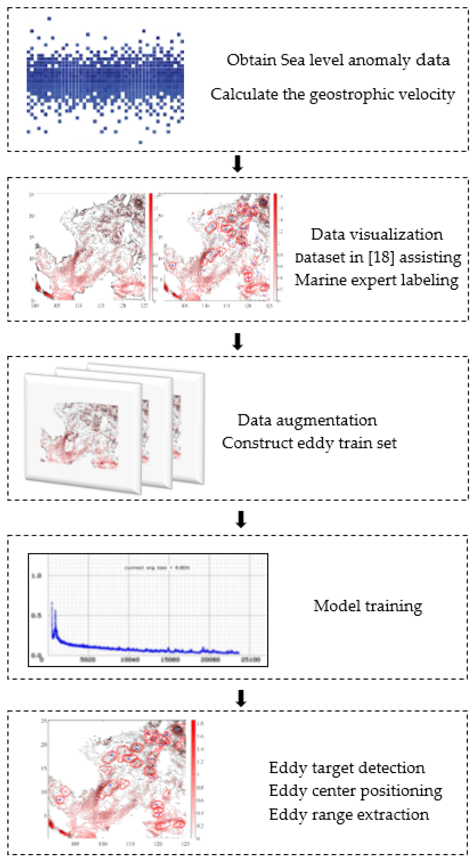
3. Outline of Our Method

The deep learning method proposed in this paper includes three stages: the preprocessing stage, the network stage, and the eddy extraction stage. The overall framework of the algorithm is shown in Figure 1. In the preprocessing stage, we preprocessed the remote sensing satellite altimeter data and enhanced the accurate small sample data to obtain the train set; in the network stage, a deep learning integration model with an object detection network as the main part was designed. In order to facilitate further study after mesoscale eddy detection, the trained model was used in the third stage to detect the eddy extent and output the eddy center coordinates and effective contour. Our method constructs a complete eddy detection system, which can efficiently utilize remote sensing data. Specific steps and innovations are described in detail in the following sections.

4. Accurate Small Sample Acquisition and Data Augmentation

4.1. Accurate Sample Acquisition

A deep learning algorithm requires a certain amount of data as support, and reasonable sample marking determines the recognition accuracy of subsequent classifiers. As described in the above section, we enhanced the data of expert labeled samples to generate a train set using digital image processing technology. The input images were generated from the SLA data processing provided by Ssalto/Duacs and distributed by the Archiving, Validation and Interpretation of Satellite Oceanographic data (AVISO), with support from the Copernicus Marine and Environment Monitoring Service (CMEMS) (http://www.aviso.altimetry.fr/duacs). The data were ‘delayed time’, ‘all sat merged’ global daily sea level anomalies on a 0.25° grid since January 1993.

The SLA data of the South China Sea (0–25°N, 100–125°E) for three years (2011–2013) were selected in the study. The data of the 1st and 15th of each month were taken as the representative of the month, providing a total of 72 NetCDF data. The data from 2012–2013 were used to generate the train set, and 2011 was set aside to test our model. The information presented to experts is shown in Figure 2, including sea level anomaly, vector field velocity, and speed of geostrophic velocity. The speed of geostrophic velocity can be calculated by the following formula:

$$\begin{gathered} u=-\frac{g}{f}\frac{\partial \xi }{\partial y},v=\frac{g}{f}\frac{\partial \xi }{\partial x} \\ \mathrm{speed}=\sqrt{\left(u^2+v^2\right)} \end{gathered}$$

(1)

where u and v represent the zonal and meridional components of the geostrophic current velocity, $g$ represents the gravitational acceleration, f is the Coriolis parameter, and ξ is the sea level anomaly.

The data are visualized with contour lines, vector lines, and color maps (Figure 2a), and the units of the interval between contours are cm. The land part must be completed with NAN values, which helps to avoid outliers and detection interference. In addition to the above information, experts can also use the daily global mesoscale ocean eddy dataset on scientific data [18] for reference during the annotation process. The target eddies in the 72 images are marked as shown in Figure 2b, where the red and blue curve indicates the eddy contour and the incomplete mesoscale eddy samples are abandoned in the marking process. The cyclone eddies are marked in blue points and blue curves, and the anticyclone eddies are marked in red points and red curves. According to Figure 2b, there are 29 mesoscale eddies in the South China Sea at this moment. In order to give readers a clear view of the data field, we provide Figure 2c, which shows the arrows and the positive and negative of the SLA. Vector arrow represents the direction of geostrophic velocity, and the solid lines and the dash lines show where the values of SLA are positive and negative, respectively.

The 2011 part of these 72 images was used as the test set, and the 2012–2013 part was used to generate the train set. The 48 maps were manually labeled, using the bounding box to mark the mesoscale eddy at the corresponding position in the image, confirming the category and generating .xml files including object information. Each map has a unique corresponding .xml file that facilitates the same change operation of the annotation data when the original image data are enhanced, eliminating the issue of re-annotating manually after data augmentation.

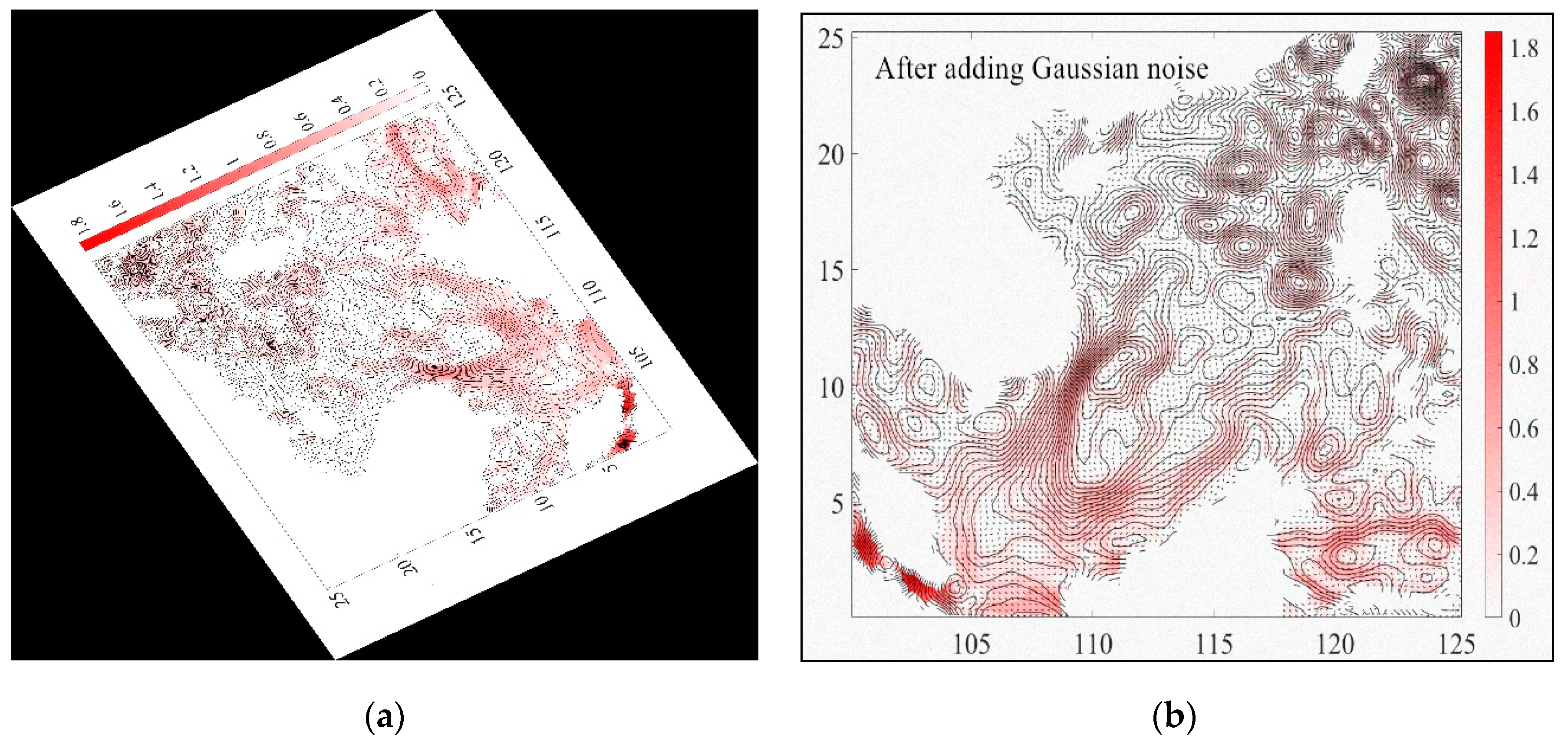
4.2. Data Augmentation

Although a few accurate mesoscale eddy samples could be obtained through labeling by marine experts, the dataset still failed to meet the requirement of the deep learning algorithm; namely, a large number of images for training. We could obtain train set through data augmentation. The rotation invariance and other characteristics of two-dimensional images enabled us to carry out a series of affine changes to expand the samples. Rotation and noise processing were performed on 48 maps with labels, which are shown in Section 4.1. Each original image was processed as follows:

(1) The 48 SLA contour maps’ size was standardized in order to facilitate the location of eddy centers at the later stage.

(2) Using the bilinear interpolation algorithm to rotate each map in the dataset, we set the rotation step size. Each SLA contour map was rotated by 30°, 60°, 90°, 120°, 150° … 300°, and 330° to obtain 11 new images, which were rotated counterclockwise and saved as the whole scaling mode. The rotated image size was standardized to 1240 × 968. At the same time, the dimensioned xml file was rotated in exactly the same way in order to obtain a set of tagged samples expanded 12 times. Thus, the 48 original images were expanded to 576 images (Figure 3a).

(3) For the 576 amplified images, we added Gaussian noise with a mean value of μ = 0 and a variance of σ = 0.0055 to each image, due to the fact that the noise of small variance is more common in natural conditions. The method of designing the variance was based on the actual noise of complex environment samples, as shown in Equation (2) as follows:

$$\mathsf{\sigma }=\frac{x^2}{m^2}$$

(2)

where m is the maximum value of the image pixel (m = 1240 in the SLA contour map) and x is the noise effect. After adding noise to each image, we got twice as many images as in step (2), with a total of 1152 images (Figure 3b).

Compared with the original maps, the maps after the process of rotation and noise addition still retained the basic characteristics. Moreover, a variety of factors were added such as scale, angle, signal-to-noise ratio, etc. Data augmentation not only increased the number of mesoscale eddy samples to reach the order of 10⁴, satisfying the requirement of the deep study, but it also added samples with noise to the train set, thus enhancing the robustness of the convolution neural network and reducing the probability of network overfitting under the condition of insufficient training samples.

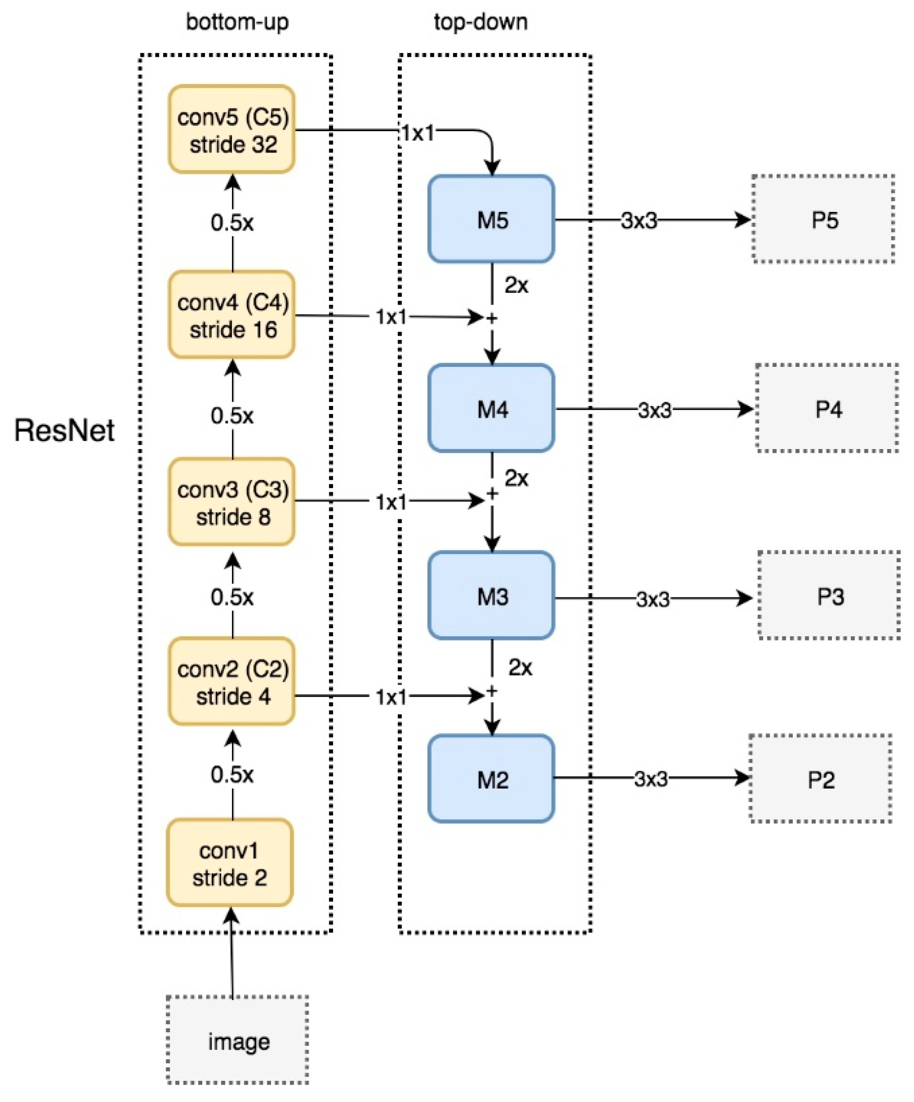
5. OEDNet Model Based on Object Detection Network

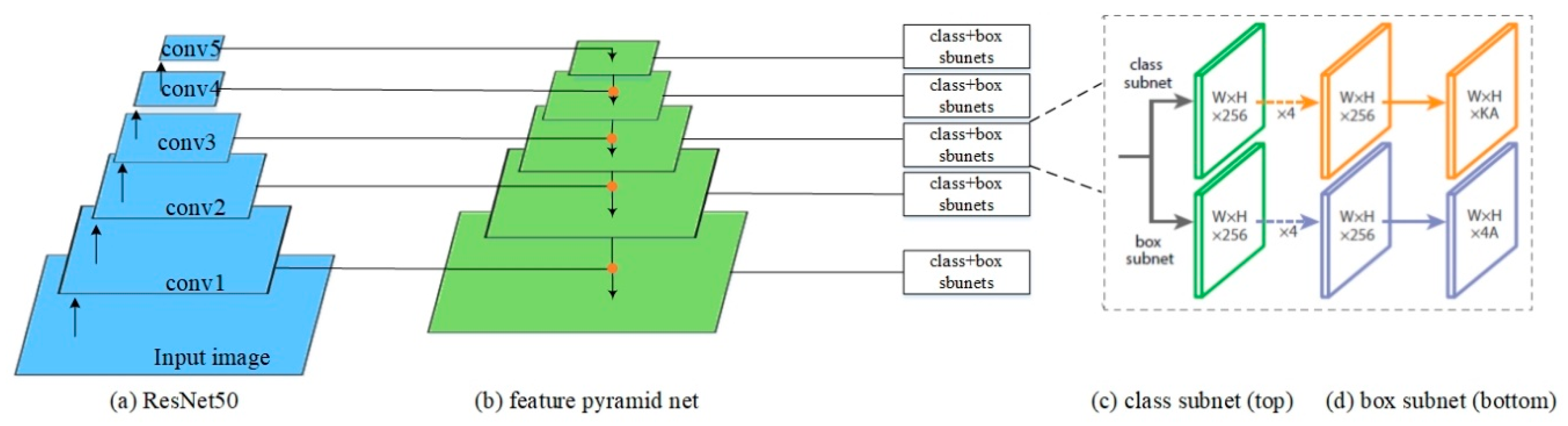
5.1. Network Structure

The object detection model we built is a multi-layer network structure called Ocean Eddy Detection Net (OEDNet), whose infrastructure is similar to the RetinaNet, a popular one-stage object detection network in deep learning. It includes two separable functions: feature extraction and object detection. Our model consists of three modules: the deep residual network (ResNet) for the initial extraction of image features, the feature pyramid network (FPN) for feature refinement extraction, and the sub-network (sub-network) for classification and positioning. Its structure is shown in Figure 4 [16].

In the field of deep learning, linear convolutional neural networks are generally adopted to extract features, such as early ImageNet and AlexNet. The residual network added into the network design in this paper can effectively avoid some disadvantages of linear Convolutional Neural Network (CNN). By adding fast connection in the convolutional feedforward network, errors and feature loss caused by the convolution and transmission of traditional CNN can be reduced, and the complexity of calculation will not be affected. Our model employs a 50-layer convolutional neural network named ResNet50 for the residual network part, and the activation function used in these convolutional layers is the correction linear element (Relu).

FPN consists of two paths, as shown in Figure 5 [16]: bottom–up and top–down. The bottom–up path is the usual convolution network for extracting features. From the bottom–up, the spatial resolution decreases, more high-rise structures are detected, and the semantic value of the network layer increases accordingly. Bottom–up is the forward propagation process of CNN. After the convolution operation of a 3 × 3 convolution kernel and a step size of 1, the first layer network structure P5 of FPN is obtained. The top–down process is carried out by up-sampling. The horizontal connection adds the result of up-sampling to the characteristic graph generated from the bottom–up, that is, the convolution operation with a 1 × 1 convolution kernel and a step size of 1 for C4 is added to the up-sampling result of P5, and then the convolution operation with a 3 × 3 convolution kernel and a step size of 1 is carried out to obtain the second layer network structure P4 of FPN. This pattern is continued with P3 and P2. The structure of FPN can effectively construct multi-scale feature maps from single images, so that each layer of the pyramid can be used for the visual detection of different sizes. In view of the simple characteristics of oceanic mesoscale eddy samples and the accurate target location, the side connection of the feature pyramid network can be used to better identify small objects.

As it is different from the network structure in [29,30], OEDNet can detect the task as a regression problem rather than a simple classification whose inputs are SLA contour maps and eddy annotation .xml files. By scanning the entire image at one time, through multiple layers of convolution processing, the network output is characteristic of the grid. These characteristics on the drawing of each small box correspond to an area of the original image. Once the frame’s position is predicted, it is simply returned to the position of the bounding box.

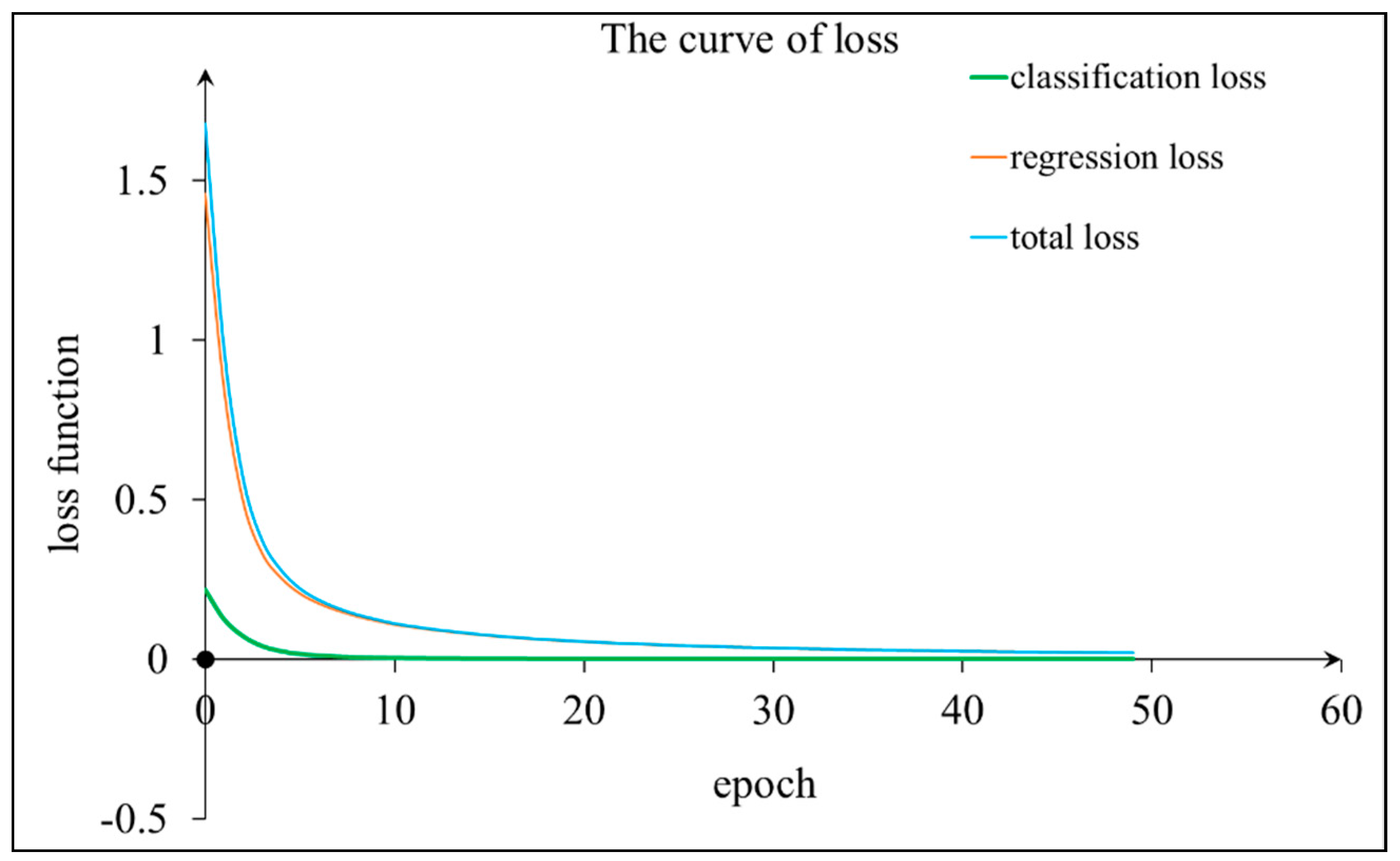
5.2. Network Training

In this paper, a Keras framework with TensorFlow backend was used to build and train the model. The experimental training and test environment were equipped with two GTX 1080Ti GPU. Taking the data prepared in Section 3 as the train set, we input the image samples and tagged files into OEDNet for training. Some specific task parameters needed additional adjustments to obtain the best performance. Lr(learning rate) refers to the magnitude of updating network weights in the optimization algorithm. Batch_size refers to the number of samples sent into the model by the neural network for each training. Epoch refers to the number of times that the entire training set was input into the neural network for training. Dropout was a way to prevent network from overfitting. In this paper, the Lr of the model was initialized to 0.001, batch_size was initialized to 100, epoch was initialized to 50, and dropout was initialized to 0.8; each epoch ran 10,000 steps, and each step ran all the input images in the network for one round completely, until the regression loss and classification loss of the network became convergent. The total training time was 67 h. The convergence curves of model training are shown in Figure 6. The total loss is the sum of the classification loss and regression loss.

For OEDNet training, we need to pay attention to three basic considerations: (1) in network construction, ResNet, FPN, and sub-network must be all connected in correct order; (2) model should be saved for every epoch to prevent network overfitting. Results are evaluated by selecting the iteration model with the best test performance. (3) When the loss function value stopped improving after five consecutive epochs, the learning process was stopped using the early stop strategy.

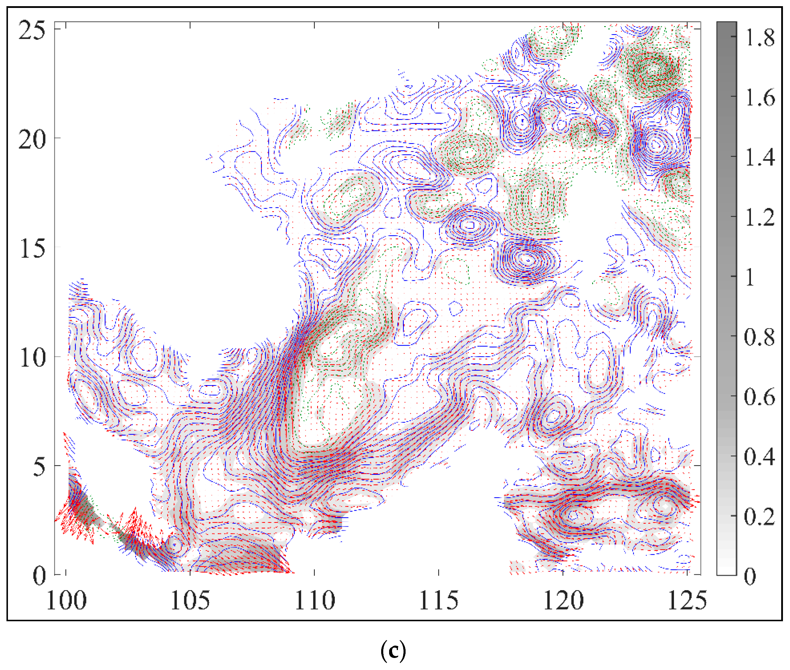
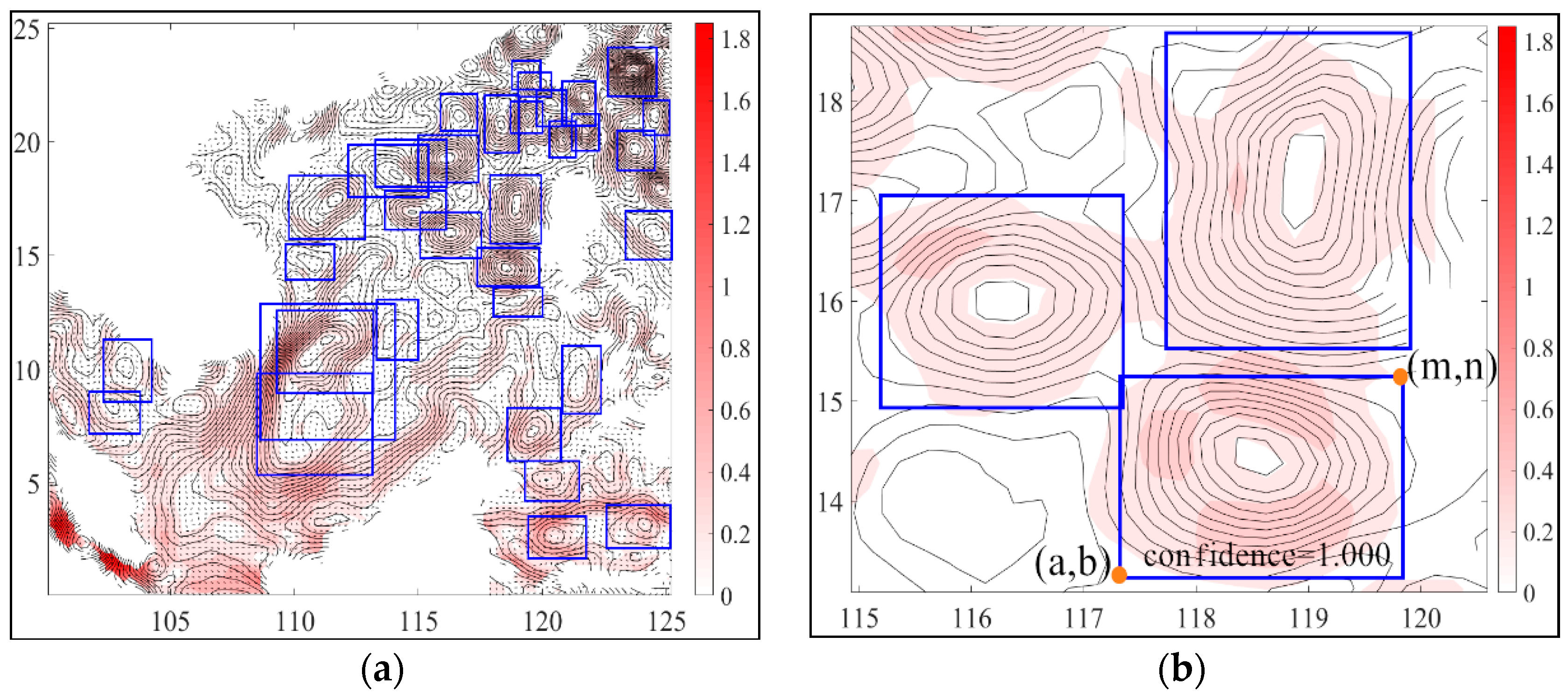
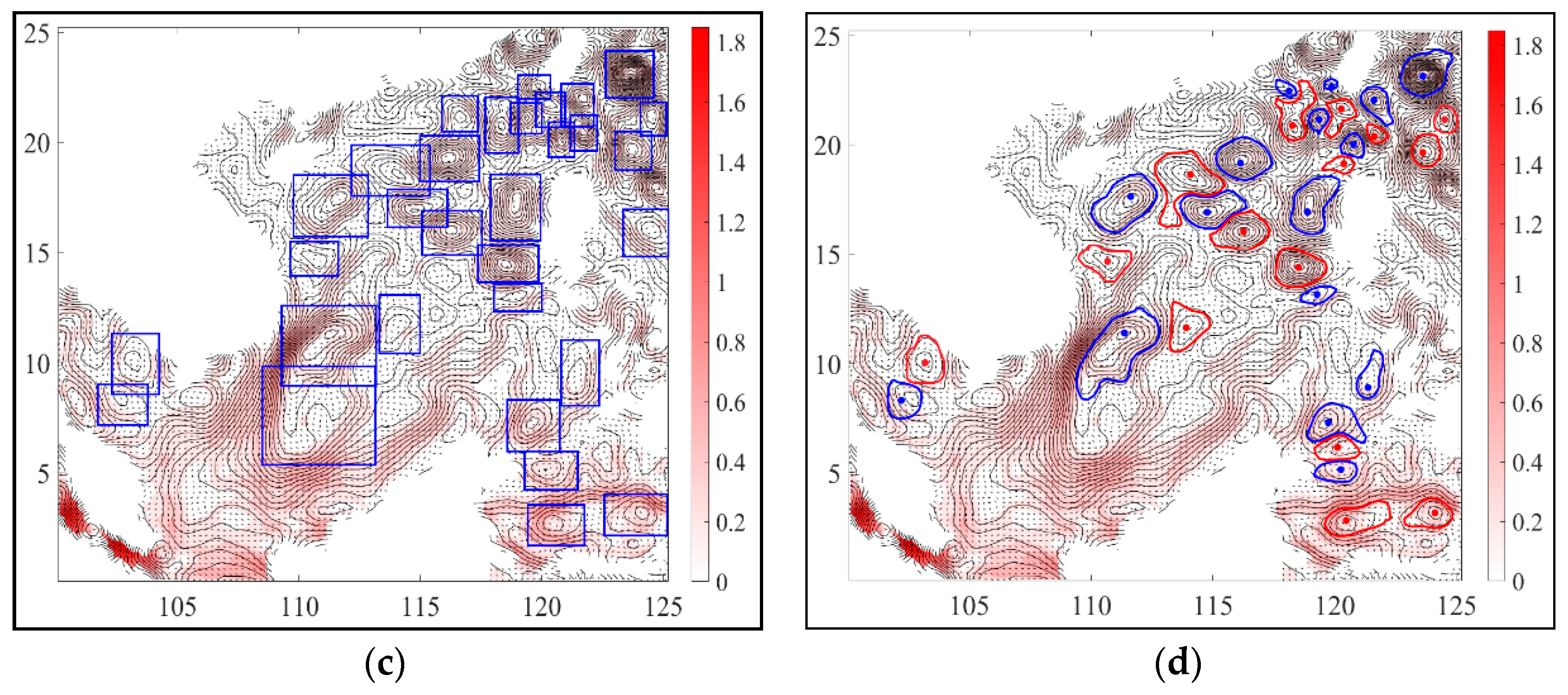
6. Eddy Center Positioning and Eddy Range Extraction

After object detection, we can obtain the results shown in Figure 7a. Each mesoscale eddy target is marked by bounding boxes, including the location and confidence of the target, the ranges of which are indicated by points as shown in Figure 7b. However, we still needed to optimize the detected targets to make the results more visible. First, we used the non-maximum suppression (NMS) algorithm [32] to eliminate overlapping bounding boxes on each detected eddy target. The intersection over union (IOU) threshold value was set at 0.4, and then all the bounding boxes were arranged according to the score from high to low values. We removed the boxes whose overlap areas were larger than 40% compared with the maximum confidence target. We repeated the above process until all overlapped boxes could be treated, ensuring that each eddy target was detected in only one box.

The results processed by the NMS algorithm are clearer than the previous step (Figure 7a) and without loss accuracy, which facilitates the next step of outputting the center and contour of each mesoscale eddy. The coordinate output of eddy center requires SLA value. We thus set the following steps:

(1) For each grid point G₀ in a bounding box, we compared its SLA value to its 24 neighbors in a 5 × 5 neighborhood. If SLA value in G₀ takes the absolute minimum/maximum within 5 × 5 neighborhood, G₀ is labeled as the extreme point.

(2) The number of extreme points is denoted as n, and the eddy center is determined by the following steps according to n.

(2.1) If n = 0, there is no extreme point. Delete this bounding box.

(2.2) If n = 1, there is only one extreme point in the range of the detected box; this point is the eddy center.

(2.3) If n > 1, there are multiple extremum points; we determine the eddy center based on the number of peripheral closure contours of the extreme points. Calculate the number of extreme points with the largest number of closed contours and denote it as m. If m = 0, there is no eddy center. Delete this bounding box. If m = 1, this point is the eddy center [33]. If m > 1, the geometric center of the bounding box is considered as the eddy center.

After the above steps, we can obtain the eddy center of all detected mesoscale eddies. The eddy region is generated based on the closed contour algorithm, and the kinds of mesoscale eddies are determined according to whether SLA around the eddy center are increasing or decreasing [18]. Since the network outputs the range of each mesoscale eddy target, we no longer needed to conduct a global search for the entire sea area grid, which saves a lot of time compared to the closed contour method. Starting from each eddy center, we set the appropriate step size and expanded the eddy range. Lastly, we obtained the coordinates of the eddy center and completed the outermost contour outputs after all the detected eddy targets were traversed.

7. Result and Discussion

In order to highlight the advantages and disadvantages of the method, the test set generated from the 2011 data was used to evaluate the results. We input the test set directly into the model and executed a series of subsequent tests, during which no manual intervention was allowed. At the same time, we selected the method widely used in related work to test the same data. Since eddies are not accurately defined, all algorithms rely on the visual interpretation of experts when evaluating the final accuracy. The experiment in this paper is carried out under the environment of i7-4.00GHzCPU and 16GB memory. Matlab is used to test all methods.

In the field of object detection and ocean eddy extraction, four typical metrics are used to measure the performance of a method: precision, recall, F_measure, and execution time [29,30]:

$$Precision=\frac{TP}{TP+FP}$$

(3)

$$Recall=\frac{TP}{P}$$

(4)

$$F_{measure}=\frac{2}{\frac{1}{precision}+\frac{1}{recall}}$$

(5)

where TP, TN denote the numbers of samples correctly marked as positive and negative, respectively; FP, FN denote the numbers of samples wrongly marked as positive and negative, respectively; P represents the actual number of targets in the sea area, namely, the number of mesoscale eddies marked by marine experts; precision represents the proportion of real samples in all identified mesoscale eddies; recall means the ratio of correctly recognized number of eddies to the number marked by experts; and F_measure represents the comprehensive evaluation value of the eddy detection algorithm. When analyzing the execution time, we neglect the training cost of OEDNet, because once the network training is finished, we can reuse it in the future recognition process. In order to compare the algorithm performance of our method with other eddy detection methods (Q-criterion, Ω-criterion, Δ-criterion, Okubo-Weiss parameter, and closed contour method) mentioned in Section 2, we analyze four typical metrics (precision, recall, F_measure, and execution time), and the comparison results are shown in

Table 1. Comparison of content related to eddy detection via multiple methods.

Methods	Recall	Precision	F-Measure	Execution Time (Sec)
Q-criterion	71.31%	65.21%	0.681	5.21
Ω-criterion	77.24%	77.51%	0.774	6.49
Δ-criterion	84.23%	39.69%	0.540	7.07
Okubo–Weiss parameter	77.13%	69.75%	0.733	3.11
Closed contour method (dataset in [18])	95.68%	85.59%	0.904	132.90
Proposed method (OEDNet)	94.61%	96.65%	0.956	7.10

.

It can be seen that OEDNet has the best overall performance. Compared with the local methods, our approach obtained higher recall and precision. The model does not rely on thresholds to avoid subjectivity. F_measure also proves that our method is obviously superior to the local method and reduces many false positive results. Compared with the closed contour method, which had the highest recall, the situation is more complex. It should be noted that although the recall of OEDNet was slightly lower than that of closed contour method, the precision was increased by 11%. It has obvious advantages when considering the comprehensive evaluation index (F_measure) and execution time. Our method reduces a large number of false identifications and saves a lot of time, ensuring that the true positive rate of mesoscale eddy detection reaches higher than 95%. It also avoids the issues of the closed isoline method, which requires a large number of secondary manual screenings.

In addition to the above results, we conducted a number of experiments to evaluate the performance of our method. We first explored the impact of data augmentation on network performance. Under the condition that network structure and network training were exactly the same, we used original maps marked by experts, images with only added noise, and images with all data augmentation methods mentioned in Section 4.2 as the train set to train three models, respectively. The test results of the three models are shown in

Table 2. Performance evaluation of the models trained by different train sets.

The Train Set of the Model	Recall	Precision	F-Measure
Original maps	89.77%	92.30%	0.910
Images only with added noise	91.67%	96.74%	0.941
Images with all data augmentation methods	94.61%	96.65%	0.956

.

It can be seen intuitively from the comparison in Table 2 that a network trained with the sample set after data augmentation detects a greater number of mesoscale eddy targets, and this directly demonstrates the effectiveness of data augmentation. The performance differences of models trained with different train sets also indicate that both rotation and adding Gaussian noise are effective data augmentation methods.

In order to test the generalization ability of OEDNet in different sea areas, the eddy detection model constructed in this paper was tested using data from other areas in 2011. We selected the same size of ocean areas for testing, including the Indian Ocean (25–50 °S, 45–70 °E), the Pacific Ocean (25–50 °N, 145–120 °W), and the Atlantic Ocean (25–50 °N, 75–50 °W). The results show that although OEDNet takes the South China Sea data as the train set, the existence of mesoscale eddies can still be detected in other sea areas. We can see from Figure 8 and

Table 3. The detection effect of the model on several different sea areas.

Sea Area	Recall	Precision	F-Measure
Indian Ocean	96.55%	98.25%	0.974
Pacific Ocean	95.31%	98.39%	0.968
Atlantic Ocean	92.59%	98.03%	0.952

that the recall of the model remained stable across different sea areas. Combined with Table 1 and Table 3, the average recall of the model in the four sea areas is more than 95% and the average of F_measure is stable at more than 0.95, which shows that our model has good eddy detection ability in different sea areas. Compared with the existing deep learning methods, whose global accuracy is 89% [21], we achieved higher accuracy. In our model, the FPN structure is included in the design, so the input image can be of any size. As long as the mesoscale eddy texture features are clearly presented in the image, OEDNet can detect them quickly and accurately.

8. Conclusions and Prospects

This paper studies the application of deep learning in ocean remote sensing data processing, that is, mesoscale eddy detection and location based on SLA contour maps. We completed the construction of a deep neural network—OEDNet—based on the object detection network. Through train set acquisition, network training, and parameter adjustment, we successfully combined mesoscale eddy automatic recognition with target detection. The innovation of the proposed method lies in data augmentation based on a small number of accurate samples marked by experts, which enabled us to solve the problem of insufficient deep learning samples. The design idea that only a linear convolution network can be used in the existing deep learning method was improved. The function of the object detection network was also made more intelligent than the existing deep learning methods [29,30], as it is no longer limited to the image classification problem but can also realize mesoscale eddy location, which will be useful for future developments in eddy tracking and trajectory prediction. Experimental results show that the method we proposed has better detection effect, shorter execution time, and good generalization ability.

One limitation of the model is that it is only suitable for AVISO satellite sea level products. Other variables, such as high resolution model SLA data [34], and sea surface temperature, can be added to improve the model and the detection results in future work. In addition, we can consider other data augmentation methods, such as adding more realistic noise [35]. At the same time, we should consider adding a time dimension to track the detected mesoscale eddy target trajectories and long short-term memory (LSTM) network to realize eddy motion prediction. Researchers could also study 3D versions of OEDNet.

References

1. Bennett, A.F.; White, W.B. Eddy heat flux in the subtropical North Pacific. J. Phys. Oceanogr. 1986, 16, 728–740. [Google Scholar] [CrossRef]
2. Roemmich, D.; Gilson, J. Eddy transport of heat and thermocline waters in the North Pacific: A key to interannual/decadal climate variability. J. Phys. Oceanogr. 2001, 31, 675–687. [Google Scholar] [CrossRef]
3. Hausmann, U.; Czaja, A. The observed signature of mesoscale eddies in sea surface temperature and the associated heat transport. Deep Sea Res. Part I Oceanogr. Res. Pap. 2012, 70, 60–72. [Google Scholar] [CrossRef]
4. Gordon, A.L.; Giulivi, C.F. Ocean eddy freshwater flux convergence into the North Atlantic subtropics. J. Geophys. Res. Ocean. 2014, 119, 3327–3335. [Google Scholar] [CrossRef]
5. Le Traon, P.; Morrow, R. Ocean currents and eddies. In International Geophysics; Elsevier: Amsterdam, The Netherlands, 2001; Volume 69, pp. 217–236. [Google Scholar]
6. Frenger, I.; Gruber, N.; Knutti, R.; Münnich, M. Imprint of Southern Ocean eddies on winds, clouds and rainfall. Nat. Geosci. 2013, 6, 608. [Google Scholar] [CrossRef]
7. Gaube, P.; Chelton, D.B.; Samelson, R.M.; Schlax, M.G.; O’Neill, L.W. Satellite observations of mesoscale eddy-induced Ekman pumping. J. Phys. Oceanogr. 2015, 45, 104–132. [Google Scholar] [CrossRef]
8. Gaube, P.; Barceló, C.; McGillicuddy, D.J., Jr.; Domingo, A.; Miller, P.; Giffoni, B.; Marcovaldi, N.; Swimmer, Y. The use of mesoscale eddies by juvenile loggerhead sea turtles (Caretta caretta) in the southwestern Atlantic. PLoS ONE 2017, 12, e0172839. [Google Scholar] [CrossRef]
9. Chaigneau, A.; Gizolme, A.; Grados, C. Mesoscale eddies off Peru in altimeter records: Identification algorithms and eddy spatio-temporal patterns. Prog. Oceanogr. 2008, 79, 106–119. [Google Scholar] [CrossRef]
10. Hinton, G.E.; Salakhutdinov, R.R. Reducing the dimensionality of data with neural networks. Science 2006, 313, 504–507. [Google Scholar] [CrossRef]
11. Weng, S.; Zhang, C.; Lin, Z. Exploring the structure of supervised data by Discriminant Isometric Mapping. Pattern Recognit. 2005, 38, 599–601. [Google Scholar] [CrossRef]
12. Bao, S.; Zhang, R.; Wang, H.; Yan, H.; Yu, Y.; Chen, J. Salinity profile estimation in the Pacific Ocean from satellite surface salinity observations. J. Atmos. Ocean. Technol. 2019, 36, 53–68. [Google Scholar] [CrossRef]
13. Zeng, X.; Li, Y.; He, R. Predictability of the loop current variation and eddy shedding process in the Gulf of Mexico using an artificial neural network approach. J. Atmos. Ocean. Technol. 2015, 32, 1098–1111. [Google Scholar] [CrossRef]
14. Girshick, R.; Donahue, J.; Darrell, T.; Malik, J. Rich feature hierarchies for accurate object detection and semantic segmentation. In Proceedings of the IEEE Conference on Computer Vision and Pattern Recognition, Columbus, OH, USA, 24–27 June 2014; pp. 580–587. [Google Scholar]
15. Chelton, D.B.; Schlax, M.G.; Samelson, R.M. Global observations of nonlinear mesoscale eddies. Prog. Oceanogr. 2011, 91, 167–216. [Google Scholar] [CrossRef]
16. Lin, T.-Y.; Goyal, P.; Girshick, R.; He, K.; Dollár, P. Focal loss for dense object detection. In Proceedings of the IEEE International Conference on Computer Vision, Venice, Italy, 22–29 October 2017; pp. 2980–2988. [Google Scholar]
17. McGillicuddy, D.J., Jr.; Robinson, A.; Siegel, D.; Jannasch, H.; Johnson, R.; Dickey, T.; McNeil, J.; Michaels, A.; Knap, A. Influence of mesoscale eddies on new production in the Sargasso Sea. Nature 1998, 394, 263. [Google Scholar] [CrossRef]
18. Faghmous, J.H.; Frenger, I.; Yao, Y.; Warmka, R.; Lindell, A.; Kumar, V. A daily global mesoscale ocean eddy dataset from satellite altimetry. Sci. Data 2015, 2, 150028. [Google Scholar] [CrossRef] [Green Version]
19. Pascual, A.; Faugère, Y.; Larnicol, G.; Le Traon, P.Y. Improved description of the ocean mesoscale variability by combining four satellite altimeters. Geophys. Res. Lett. 2006, 33. [Google Scholar] [CrossRef] [Green Version]
20. Jiang, M.; Machiraju, R.; Thompson, D. Detection and Visualization of Vortices. In The Visualization Handbook; Elsevier: Amsterdam, The Netherlands, 2005; p. 295. [Google Scholar]
21. Okubo, A. Horizontal dispersion of floatable particles in the vicinity of velocity singularities such as convergences. Deep Sea Res. Oceanogr. Abstr. 1970, 17, 445–454. [Google Scholar] [CrossRef]
22. Weiss, J. The dynamics of enstrophy transfer in two-dimensional hydrodynamics. Phys. D Nonlinear Phenom. 1991, 48, 273–294. [Google Scholar] [CrossRef]
23. Hunt, J. Vorticity and vortex dynamics in complex turbulent flows. Trans. Can. Soc. Mech. Eng. 1987, 11, 21–35. [Google Scholar] [CrossRef]
24. Liu, C.; Wang, Y.; Yang, Y.; Duan, Z. New omega vortex identification method. Sci. China Phys. Mech. Astron. 2016, 59, 684711. [Google Scholar] [CrossRef]
25. Chong, M.S.; Perry, A.E.; Cantwell, B.J. A general classification of three-dimensional flow fields. Phys. Fluids A Fluid Dyn. 1990, 2, 765–777. [Google Scholar] [CrossRef]
26. Jeong, J.; Hussain, F. On the identification of a vortex. J. Fluid Mech. 1995, 285, 69–94. [Google Scholar] [CrossRef]
27. McWilliams, J.C. The emergence of isolated coherent vortices in turbulent flow. J. Fluid Mech. 1984, 146, 21–43. [Google Scholar] [CrossRef] [Green Version]
28. Chen, G.; Han, G.; Yang, X. On the intrinsic shape of oceanic eddies derived from satellite altimetry. Remote Sens. Environ. 2019, 228, 75–89. [Google Scholar] [CrossRef]
29. Ashkezari, M.D.; Hill, C.N.; Follett, C.N.; Forget, G.; Follows, M.J. Oceanic eddy detection and lifetime forecast using machine learning methods. Geophys. Res. Lett. 2016, 43, 12234–12241. [Google Scholar] [CrossRef]
30. Lguensat, R.; Sun, M.; Fablet, R.; Tandeo, P.; Mason, E.; Chen, G. EddyNet: A deep neural network for pixel-wise classification of oceanic eddies. In Proceedings of the IGARSS 2018-2018 IEEE International Geoscience and Remote Sensing Symposium, Valencia, Spain, 22–27 June 2018; pp. 1764–1767. [Google Scholar]
31. Xu, G.; Cheng, C.; Yang, W.; Xie, W.; Kong, L.; Hang, R.; Ma, F.; Dong, C.; Yang, J. Oceanic Eddy Identification Using an AI Scheme. Remote Sens. 2019, 11, 1349. [Google Scholar] [CrossRef]
32. Neubeck, A.; Van Gool, L. Efficient non-maximum suppression. In Proceedings of the 18th International Conference on Pattern Recognition (ICPR’06), Hong Kong, China, 20–24 August 2006; pp. 850–855. [Google Scholar]
33. Zhang, W.-Z.; Ni, Q.; Xue, H. Composite eddy structures on both sides of the Luzon Strait and influence factors. Ocean Dyn. 2018, 68, 1527–1541. [Google Scholar] [CrossRef]
34. Amores, A.; Jordà, G.; Arsouze, T.; Le Sommer, J. Up to what extent can we characterize ocean eddies using present-day gridded altimetric products. J. Geophys. Res. Ocean. 2018, 123, 7220–7236. [Google Scholar] [CrossRef]
35. Klyatskin, V.; Koshel, K. Impact of diffusion on surface clustering in random hydrodynamic flows. Phys. Rev. E 2017, 95, 013109. [Google Scholar] [CrossRef]
Figure 1. The flow chart of the proposed mesoscale eddy detection algorithm based on deep learning.
Remotesensing 11 01921 g001
Figure 2. (a) Maps to be labeled by experts and the input set of the network. (b) The contours of mesoscale features identified by domain experts. (c) The visualization of SLA and geostrophic velocity. Color map and contours (black lines) represent the geostrophic velocity speed [m/s] (Equation (1)), and sea level anomaly [cm], respectively.
Remotesensing 11 01921 g002aRemotesensing 11 01921 g002b
Figure 3. (a) An example of the original image rotation by 120°. (b) The SLA contour map after adding Gaussian noise. Color map and contours (black lines) represent the geostrophic velocity speed [m/s] (Equation (1)) and sea level anomaly [cm] respectively.
Remotesensing 11 01921 g003
Figure 4. The network structure.
Remotesensing 11 01921 g004
Figure 5. The connection between feature pyramid network (FPN) and ResNet50.
Remotesensing 11 01921 g005
Figure 6. Curves of classification loss (green line), regression loss (orange line), and total loss (light blue line) as a function of epoch.
Remotesensing 11 01921 g006
Figure 7. (a) The raw output of the model built in this paper; (b) example for the output of bounding box; (c) the eddy detection results processed by the non-maximum suppression (NMS) algorithm; and (d) the final visualization result after eddy center positioning and contour output (the cyclone eddies are marked in blue points and blue curves, and the anticyclone eddies are marked in red points and red curves). Color map and contours (black lines) represent the geostrophic velocity speed [m/s] (Equation (1)) and sea level anomaly [cm], respectively.
Remotesensing 11 01921 g007aRemotesensing 11 01921 g007b
Figure 8. The eddies detected by Ocean Eddy Detecion Net (OEDNet) in different sea areas. (a) Indian Ocean, (b) Pacific Ocean, and (c) Atlantic Ocean. Color map and contours (black lines) represent the geostrophic velocity speed [m/s] (Equation (1)) and sea level anomaly [cm], respectively.
Remotesensing 11 01921 g008