Estimating Subsurface Thermohaline Structure of the Global Ocean Using Surface Remote Sensing Observations

Abstract

Retrieving multi-temporal and large-scale thermohaline structure information of the interior of the global ocean based on surface satellite observations is important for understanding the complex and multidimensional dynamic processes within the ocean. This study proposes a new ensemble learning algorithm, extreme gradient boosting (XGBoost), for retrieving subsurface thermohaline anomalies, including the subsurface temperature anomaly (STA) and the subsurface salinity anomaly (SSA), in the upper 2000 m of the global ocean. The model combines surface satellite observations and in situ Argo data for estimation, and uses root-mean-square error (RMSE), normalized root-mean-square error (NRMSE), and R² as accuracy evaluations. The results show that the proposed XGBoost model can easily retrieve subsurface thermohaline anomalies and outperforms the gradient boosting decision tree (GBDT) model. The XGBoost model had good performance with average R² values of 0.69 and 0.54, and average NRMSE values of 0.035 and 0.042, for STA and SSA estimations, respectively. The thermohaline anomaly patterns presented obvious seasonal variation signals in the upper layers (the upper 500 m); however, these signals became weaker as the depth increased. The model performance fluctuated, with the best performance in October (autumn) for both STA and SSA, and the lowest accuracy occurred in January (winter) for STA and April (spring) for SSA. The STA estimation error mainly occurred in the El Niño-Southern Oscillation (ENSO) region in the upper ocean and the boundary of the ocean basins in the deeper ocean; meanwhile, the SSA estimation error presented a relatively even distribution. The wind speed anomalies, including the u and v components, contributed more to the XGBoost model for both STA and SSA estimations than the other surface parameters; however, its importance at deeper layers decreased and the contributions of the other parameters increased. This study provides an effective remote sensing technique for subsurface thermohaline estimations and further promotes long-term remote sensing reconstructions of internal ocean parameters.

1. Introduction

In recent years, rapid warming has occurred in the global climate system. Meanwhile, the strongest El Niño event in the past 60 years occurred in the central and eastern Pacific with a Nino 3.4 index of up to 3.1 °C, which had a large impact on the global climate and environment [1,2]. As an area sensitive to global climate change, the ocean plays an important role in regulating the global climate system. Numerous studies have suggested that most of the heat gained by the Earth system is stored in the ocean, which leads to significant global ocean warming [3]. In particular, the heat variation and redistribution in the global subsurface and deeper ocean (300–2000 m) is of great significance to global climate change [4,5,6,7], but there are large uncertainties and discrepancies in the deeper ocean warming evaluation [8]. The ocean thermohaline structure as the indispensable environmental factors can be used to study ocean processes and climate change. Evaluating the temperature and salinity distributions within the ocean can provide a valuable basis for studying ocean dynamics and other phenomena. The ocean temperature, along with the salinity, is required to compute the ocean water density [9].

Current internal ocean observation data, while precise, are sparse in time and space and far from meeting observational requirements for multi-scale ocean process studies [8,10]. At the same time, the profile data of temperature and salinity in the ocean are sparse and their observations are extremely uneven, hindering our understanding of important dynamic processes within the ocean. The dynamic processes in the ocean interior are complex with multi-dimensional and multi-scale features; therefore, understanding such processes require well-sampled internal ocean observation data over large scales.

So far, satellite sensors have provided abundant time-series and large-scale remote sensing data with high temporal and spatial resolution. Even though remote sensing techniques have made great achievements in the marine field, the observations are still limited to the ocean’s surface and are unable to directly detect information inside the ocean. However, sea surface features can reflect the dynamic phenomena within the ocean and most interior ocean processes have sea surface manifestations [11]. Moreover, subsurface dynamic information, such as the thermohaline structure, depends greatly on many processes in the surface layer, such as the surface heat exchange, wind-driven mixing, and advection [12]. Therefore, it is feasible to retrieve pivotal subsurface dynamic information, e.g., the thermohaline structure, indirectly by combining multiple sea surface parameters from satellite observations with in situ measurements of the ocean’s interior.

Currently, with the development of satellite observations and in situ Argo datasets, more and more studies have attempted to retrieve and reconstruct important subsurface information, such as the thermohaline structure, by establishing dynamic models, empirical statistical models, or data assimilations [13]. The Bluelink Reanalysis (BRAN) model can be applied to retrieve the ocean eddy currents by assimilating satellite altimetry data, sea surface temperature (SST), and in situ data [14]. Wang et al. [15] proposed a new dynamic method, the internal plus surface quasi-geostrophic equation, which was used to retrieve the subsurface density and velocity fields on regional scales [16,17]. However, dynamic models are more suited to regional scales and rely excessively on input parameters. In addition, it is difficult to obtain large-scale and quasi-real-time sea subsurface environmental information via data assimilation. Altimetry height, combined with broad scale profile data, can be used to estimate steric height, heat storage, and subsurface temperature variability [18]. An empirical method was developed to estimate 3D oceanic thermal structures from quasi-real-time satellite altimeter data [19]. The 3D temperature and salinity fields were derived from remote sensing and in situ data [20,21]. Dynamic topography data, combined with the gravest empirical mode, can obtain time series of temperature and salinity fields [22]. Satellite altimetry was adopted to estimate the 4D temperature, salinity, and velocity fields of the Southern Ocean [23]. The global 3D geostrophic ocean circulation can be estimated based on satellite data and in situ measurements [24]. A time series of the subsurface temperature structure in the North Atlantic Ocean was derived via a self-organized map (SOM) by combining the sea surface temperature (SST) and sea surface height (SSH) [25]. Subsurface velocity fields can be retrieved from sea surface parameters, combined with geographic reference information, using the iteration self-organized map approach [26]. Salinity profiles can be estimated from surface satellite observations using a generalized regression neural network with the fruit fly optimization algorithm method [27]. The vertical profiles of chlorophyll-a can be retrieved from satellite observations using hidden Markov models and self-organizing topological maps [28]. An objective algorithm was proposed to reconstruct the 3D ocean temperature field based on Argo profiles and SST data [29]. Su et al. [30,31] and Li et al. [32] employed classic machine learning methods, such as support vector regression (SVR) and random forest (RF), to retrieve the subsurface temperature anomaly (STA) based on multi-source satellite observations, and the results showed that the models have good performance and RF outperforms SVR for global applications. The geographically weighted regression model shows a great potential for subsurface modeling with surface data, and has a significant improvement over the ordinary linear regression model by considering the significant spatial nonstationarity feature in the ocean [33].

Because the dynamic processes within the ocean are complex and nonlinear [34], it is necessary to introduce nonlinear machine learning models to reconstruct the ocean interior. In particular, ensemble learning methods are appropriate for estimating the subsurface thermohaline structure since they can promote the ability of a model to be generalized by increasing the number of base learners. This study proposes an ensemble learning algorithm, an improved gradient boosted decision tree (GBDT) algorithm, called extreme gradient boosting (XGBoost), to detect thermohaline anomalies within the global ocean (in the upper 2000 m) in different seasons of 2015. In addition, this study analyzes the estimation accuracy of the model, evaluates the reliability and stability of the model with respect to the seasons, and further analyzes the spatial distribution of the model estimation errors.

2. Study Area and Data

In this study, the global ocean (in the range of 180° W–180° E and 78.375° S–77.625° N) is the study area. The data used in this study included sea surface data (sea surface height, temperature, salinity, and wind) from satellite observations and Argo in situ data of the ocean interior. The sea surface height (SSH) data were derived from Archiving, Validation and Interpretation of Satellite Oceanographic (AVISO) altimetry [35], and the SST data were derived from the Advanced Microwave Scanning Radiometer 2 (AMSR2) sensor [36]. The sea surface salinity data were obtained from the Microwave Imaging Radiometer with Aperture Synthesis (MIRAS) sensor on the Soil Moisture and Ocean Salinity (SMOS) satellite [37]. The sea surface wind data (SSW, including the northward component (USSW) and the eastward component (VSSW)) were obtained from the Cross-Calibrated Multi-Platform (CCMP) product [38]. All the surface data were registered at monthly intervals and had a spatial resolution of 0.25°. The Argo in situ data contained 27 vertical standard levels of the ocean interior (from the surface to a depth of 2000 m), and each depth level included temperature, salinity, and other important parameters of the ocean interior [39]. The spatial resolution of the Argo data was 1°.

We unified all the datasets to the same spatial and temporal resolution (1°, monthly) first and then subtracted the climatological field from the sea surface data and Argo data to obtain their anomalies. The climatology of each variable (the base period was 2005–2016) used in this study was from the Argo gridded dataset [39]. The sea surface height anomaly (SSHA), sea surface temperature anomaly (SSTA), sea surface salinity anomaly (SSSA), northward component of the SSW speed anomaly (USSWA), and eastward component of the SSW speed anomaly (VSSWA) ranged from −0.3 m to 0.4 m, from −6 °C to 5 °C, from −2 psu to 1.5 psu, from −6 m/s to 7 m/s, and from −4 to 5 m/s, respectively, in October 2015. Finally, we normalized all the data to the range of [0, 1], so they could be used as model input parameters to make the model more reliable. These surface parameters all show significant spatial variation and heterogeneity characteristics.

3. Methods

3.1. Extreme Gradient Boosting (XGBoost)

GBDT is an iterative decision trees algorithm proposed by Jerome Friedman [40]. GBDT, as a type of boosting algorithm, is composed of multiple decision trees, where each decision tree trains the residual error of the prediction result of the last decision tree. The final result of the algorithm is obtained by summing up the results of all the decision trees.

Extreme gradient boosting (XGBoost) is an advanced version of the GBDT algorithm [41]. In addition to the first derivative, XGBoost introduces the second derivative of the error function at each data point to optimize the loss function. Meanwhile, the algorithm takes the complexity of the tree model as a regularization term in the objective function to avoid over-fitting by adding the regular terms to the cost functions. In addition, XGBoost refers to the ideas of an RF [42] during model training. This means that each iteration process does not apply all the samples and all the features of the samples but selectively takes part of the samples and part of the features for training so as to effectively improve the generalization ability of the model and weaken the under-fitting and over-fitting phenomena. The algorithm can automatically select the fraction of columns and observations to be randomly sampled for training according to certain tuned hyper-parameters such as “colsample_bytree” and “subsample.” To improve the running speed, the XGBoost algorithm also supports parallel computing. The procedure of this algorithm is to first divide the original dataset into multiple sub-datasets, and then, to randomly assign each subset to the base learner for prediction and calculate the result of the weak learner according to a certain weight. Finally, the model results can be expressed as the weighted sum of the predicted results of all the decision trees.

Parameter tuning is imperative during modeling. As a learning algorithm, XGBoost includes some hyper-parameters that cannot be directly learned from model input and training; instead, these parameters are related to the complexity and regularization of the model [43], and need to be optimized to refine the model. In this study, we employed Bayesian optimization to tune the hyper-parameters of XGBoost. This optimization method is a Gaussian process and constantly updates the prior knowledge by considering the previous parameter information, whereas a conventional grid search or random search considers no prior parameter information. In addition, the Bayesian optimization process uses a small number of iterations and has a rapid running speed, allowing it to optimize algorithms with multiple parameters such as XGBoost.

Table 1. The meaning and optimal values of some hyper-parameters of the XGBoost model.

Some Hyper-Parameters	Meaning (Default Values)	Optimal Values
learning_rate	Makes the model more robust by shrinking the weights on each step (0.3)	0.1
min_child_weight	The minimum sum of weights of all observations required in a child (1)	2
max_depth	The maximum depth of a tree (6)	16
colsample_bytree	The fraction of columns to be randomly sampled for each tree (1)	0.8
subsample	The fraction of observations to be randomly sampled for each tree (1)	0.8
gamma	The minimum loss reduction required to make a split (0)	0
reg_alpha	L1 regularization term on weights (0)	0.1
reg_lambda	L2 regularization term on weights (1)	10

shows some imperative hyper-parameters of XGBoost models tuned by the Bayesian optimization. The other parameters are set to the default values.

The XGBoost algorithm has been widely used in various fields such as remote sensing classification [44] and object detection [45]; this study attempts to use this method to estimate the thermohaline structure of the interior of the global ocean.

3.2. Experimental Setup

This study used sea surface parameters from satellite observations (i.e., the SSTA, SSHA, SSSA, USSWA, and VSSWA) to estimate the interior ocean thermohaline structure (STA and SSA) via the GBDT and XGBoost methods.

The modeling process was divided into three steps. First, the training dataset was built. The surface remote sensing parameters were selected as independent input variables of the model, and the subsurface temperature and salinity anomalies (STA and SSA) measured by Argo were used as training labels and testing labels. Meanwhile, all datasets were normalized and randomly sampled into a training set (60%) and a testing set (40%), which were used to train and test the model, respectively. Second, the XGBoost model was trained. We tuned the hyper-parameters of the XGBoost model using the Bayesian hyper-parameter optimization method, and then an appropriate XGBoost model was built with the optimal parameters combination. Third, STA and SSA were predicted using the XGBoost model. We estimated the results with the trained XGBoost model and evaluated the model accuracy via R², the root-mean-square error (RMSE), and the normalized root-mean-square error (NRMSE). Figure 1 presents the modeling process; the process for GBDT is similar to that for XGBoost.

4. Results

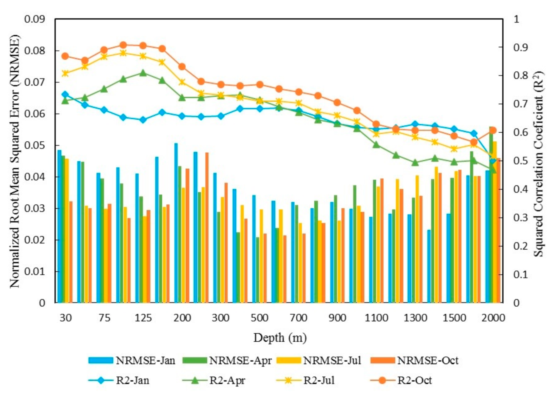
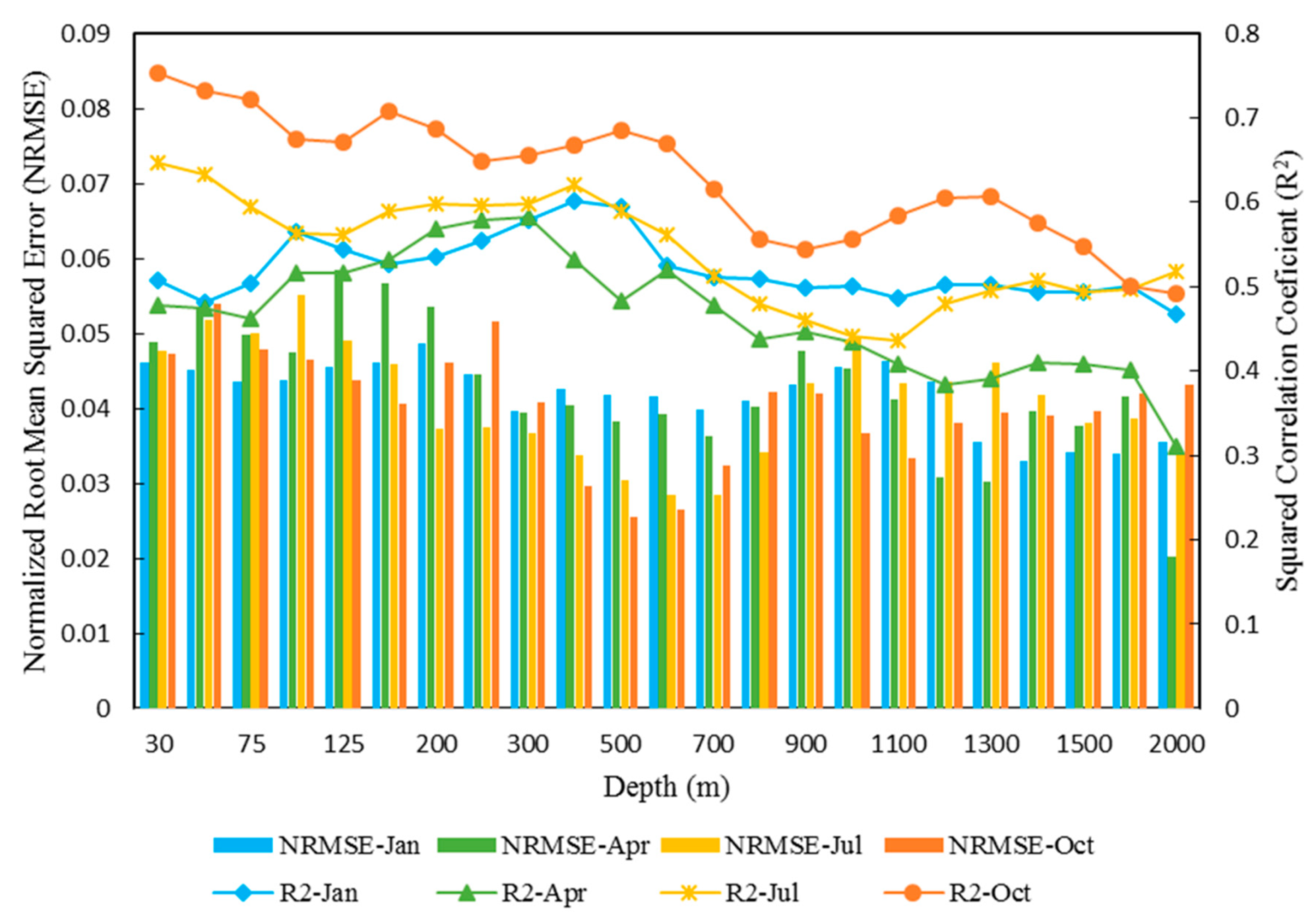
4.1. Accuracy Comparison between the XGBoost and GBDT Models

Here, in order to obtain a more reliable model with a higher accuracy, we employed the XGBoost and GBDT methods to establish regression models to estimate the thermohaline structure at 23 different depth levels (0–2000 m) in the global ocean interior for the four seasons (January (winter), April (spring), July (summer), and October (autumn)) of 2015 and to allow for a comparison between the two methods using values of the RMSE.

The average RMSE over the different depth levels in each season for the model evaluation are shown in Figure 2. The average RMSEs of the XGBoost-estimated STA and SSA at different depth levels were lower than the GBDT-estimated values, which suggests that XGBoost is better suited for estimating STA and SSA with higher accuracy at the global scale than GBDT, regardless of the season. Therefore, we selected the better model, XGBoost, as the estimation model in the following analyses. Moreover, to examine the applicability of the model, we analyzed the seasonal–spatial variation of the estimated results and investigated the model stability via a spatial distribution analysis of the estimation errors.

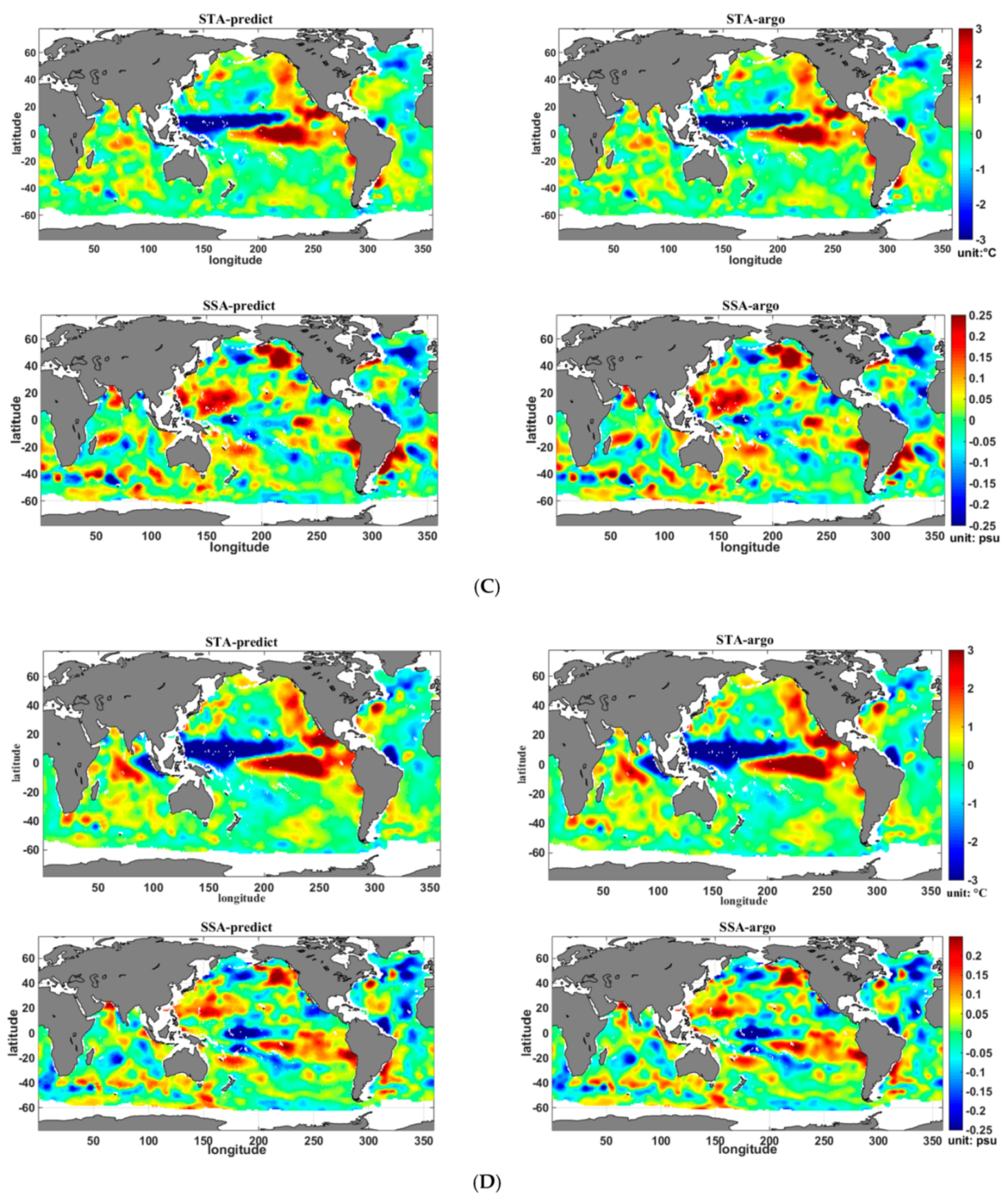
4.2. Analysis of the Seasonal Results

Figure 3, Figure 4 and Figure 5 show the spatial distribution of the thermohaline anomalies (including STA and SSA) of the global ocean interior from the XGBoost-estimated results and the Argo data in the four seasons of 2015 at several depth levels (100 m (Figure 3), 500 m (Figure 4), and 1500 m (Figure 5)). It is clear that at the same depth level, the XGBoost-estimated STA and SSA were consistent with the Argo STA and SSA. On the whole, the thermohaline anomaly signals became weaker with depth, which might be related to the weaker dynamic processes and more stable seawater stratification in the deeper layers compared to the upper layers. Moreover, the thermohaline anomalies present some similar patterns in different seasons.

As Figure 3 shows, at 100 m, the STAs were all significantly positive in the central and eastern equatorial Pacific and negative in the western equatorial Pacific in the different seasons, while the SSAs show a comparatively even distribution pattern. The global ocean STAs were dominated by the strong El Niño phenomenon at the upper depth levels in 2015. At the same time, the temperature in the western equatorial Pacific Ocean was abnormally low, and the STA in the Indian Ocean presented a distribution pattern with positive values in the east and negative values in the west because the Indian Ocean dipole was in a positive phase period. Moreover, the El Niño phenomenon in the equatorial Pacific became increasingly stronger, with a Nino 3.4 index of 0.6 °C in January, 0.8 °C in April, 1.5 °C in July, and 2.4 °C in October. Meanwhile, the SSA became increasingly significant with the seasons, presenting negative values in the western equatorial Pacific and positive values in the eastern equatorial Pacific, similar to the STA in October. This was because most of the distinctive thermohaline anomaly patterns in the subsurface ocean were dominated by the El Niño in the tropical ocean.

At depths below 500 m (in the deeper ocean), the El Niño phenomenon became weaker and the negative anomaly in the western Pacific was much weaker or even diminished at 500 m, even though there remained a high anomaly in the eastern Pacific Ocean. For both the STA and SSA patterns, the signals in the Southern Ocean and Atlantic Ocean were more intense and significant than those in the central ocean basin, possibly due to the strong boundary current and mesoscale eddy processes in the deeper ocean such as the Antarctic Circumpolar Current (ACC), Gulf Stream, and Kuroshio Current. The STA and SSA signals had little seasonal variation but both showed a latitudinal alternation distribution over the Southern Ocean and the northern Atlantic Ocean. From depths of 1000 m to 2000 m, there were almost no El Niño-Southern Oscillation (ENSO) signals and the thermohaline anomaly signals got weaker and less distinct in their spatial heterogeneity. The ranges of STA and SSA both decreased, and the anomaly patterns presented little seasonal variation in the different seasons; this was related to the significant difference in the dynamic processes between the deeper and upper layers of the ocean.

Our quantitative evaluation of the performance measures for the XGBoost STA and SSA estimations at the 23 different depth levels for the different seasons in 2015 (January, April, July, and October) according to the NRMSE and R² results is shown in Figure 6 and Figure 7. The RMSE visually reflects the true errors of the STA and SSA estimations at each depth level. The RMSE ranges of the model also varied with depth and were smaller at deeper levels due to the smaller magnitude and variance of the STA and SSA at depth. To describe the model accuracy with increasing depth more intuitively and to improve the comparability of the model accuracy at the different depth levels, we normalized the RMSE values to the relative error (NRMSE is the RMSE divided by the range of the Argo-measured STA and SSA values at the current depth level).

On the whole, both for the STA and SSA estimations, the NRMSE in the different seasons generally showed first a downtrend and then an uptrend with a turning point occurring at a depth of approximately 500 m or 600 m. The R² value first fluctuated and then showed a downtrend. This indicates that the prediction performance of the XGBoost model decreased with depth, which may be due to the relatively stable seawater stratification in the deeper layer and because deeper ocean phenomena have weaker surface manifestations, which are harder to interpret from satellite measurements. This result is consistent with the almost absent mesoscale signal shown in Figure 4 and Figure 5 at these deeper levels. In addition, at depths less than 250 m, the accuracy fluctuated due to the unstable dynamic environment in the upper ocean.

For the STA estimation, the average NRMSE and R² values of the 23 depth levels were 0.037, 0.036, 0.035, and 0.033; and 0.647, 0.652, 0.702, and 0.742 for January, April, July, and October, respectively. The model accuracy increased gradually as the seasons progressed, accompanying the stronger ENSO signal in the upper ocean. For the SSA estimation, the average NRMSE and R² values of the 23 depth levels were 0.042, 0.043, 0.041, and 0.040; and 0.521, 0.468, 0.542, and 0.629 for January, April, July, and October, respectively. The lowest accuracy occurred in April, and the highest accuracy occurred in October. The accuracy of the SSA estimation was lower in general than the STA estimation. The model accuracy was relatively high for all four seasons, suggesting that the XGBoost method had a good seasonal applicability to global STA and SSA estimations.

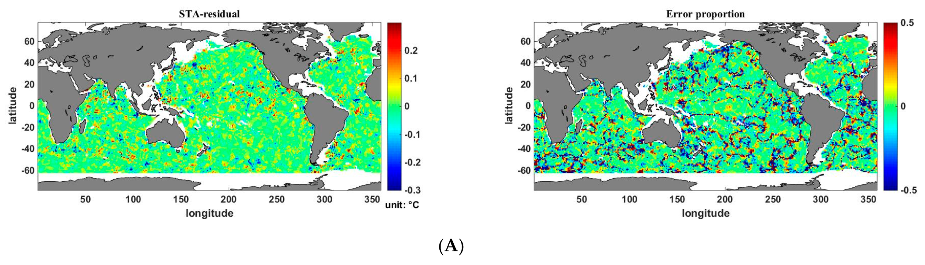
4.3. Estimation Error Analysis

The above results suggest that the STA and SSA estimation accuracies from the XGBoost model in January and April, respectively, were the lowest of the four seasons; therefore, the spatial distribution of the STA and SSA estimation errors in these respective seasons are analyzed and discussed here. The XGBoost-estimated STA and SSA values minus the Argo-measured STA and SSA values refer to the estimation errors (“STA-residual” refers to XGBoost-estimated STA minus the Argo-measured STA), which are shown in Figure 8 and Figure 9. In order to show the relative errors of the estimated STA and SSA more intuitively, we also present the error proportion (“error proportion” refers to the proportion of the estimation residual in the Argo-measured thermohaline anomaly values at each point) for STA and SSA in Figure 8 and Figure 9, respectively.

Figure 8 and Figure 9 show the spatial distributions of the XGBoost-estimated STA and SSA errors, respectively, at depths of (A) 100 m, (B) 500 m, and (C) 1500 m. On the whole, most of the error spatial distributions showed green with values close to zero; that is, the model-predicted STA and SSA values were close to the Argo values, which indicates that the XGBoost method is reliable and robust for STA and SSA estimations at the global scale in the different seasons. In the upper layer of the ocean (at the depth of 100 m), the abnormal ENSO signal in the equatorial Pacific Ocean was not well estimated and reduced the STA estimation accuracy of the model, whereas the SSA estimation error had a relatively even distribution. In addition, significant STA and SSA estimation errors occurred at the boundary of the ocean basins, such as in the Antarctic Circumpolar Current, Gulf Stream, and Kuroshio Current regions (i.e., regions including strong current dynamic processes with intense mesoscale eddy processes). There was an obvious alternation in the STA and SSA overestimation and underestimation in the Atlantic Ocean and the Southern Ocean. In the deeper layers (below 500 m), such as 1500 m, the STA and SSA estimation errors became more significant than the errors at 500 m. The estimation errors became more obvious with depth (below 100 m) since the upper thermohaline anomaly was more predictable from the surface signatures than the deeper ocean, which is in accordance with the results above. Moreover, the spatial distribution of the error proportion (relative error) is also clearly shown in Figure 8 and Figure 9. In general, the most significant error proportion showed a linear distribution, and the error proportion of SSA estimation was more significant than STA. As the depth increased, the error proportion became more distinct for both STA and SSA estimation.

4.4. Relative Importance of the Sea Surface Parameters

Previous studies have introduced some machine learning methods in this field, but have not analyzed the feature sensitivity or contribution to the estimation models [30,31,46]. To evaluate the contribution of each sea surface parameter to the estimation model, we calculated the relative importance of each parameter using the feature importance scores obtained from the getfscore function in Python. The getfscore function evaluates a feature’s score by computing the number of times a feature is used to split the data across all trees, the average gain of the feature, and the average coverage of the feature when it is used in trees.

Figure 10 and Figure 11 show the relative importance of the five surface parameters from seasonal and vertical depth perspectives, respectively, for the (a) STA and (b) SSA estimation models. The relative importance of the five surface parameters adds up to 1 for each model case. In general, all five parameters had similar feature importance (approximately 0.2), which illustrates that the surface parameters used in this study were all effective and reasonable in the XGBoost estimation model. Nevertheless, the surface wind speed anomalies (including the northward component, USSWA, and the eastward component, VSSWA) contributed relatively more than the other parameters.

The relative importance of the five parameters in the different seasons at the same depth (1000 m) were similar, which suggests that the contributions of the surface features to the model remained relatively stable with the seasons (Figure 10). Figure 11 presents the feature importance at different depth levels (100 m, 500 m, 1000 m, 1500 m, and 2000 m) in January. The surface wind speed anomalies played the most significant role in the models for both the STA and SSA estimations, regardless of the depth level. Further, from the upper layer (100 m) to the middle (500 m and 1000 m) and deep (1500 m and 2000 m) layers, the relative importance of SSHA, SSTA, and SSSA increased gradually while the importance of the u and v wind speed components decreased slightly. SSTA made a greater contribution than SSHA and SSSA to the STA estimation. Meanwhile, SSHA made a larger contribution than SSTA and SSSA to the SSA estimation.

5. Discussion

Compared to the well-performed random forest (RF) model proposed recently [31], the XGBoost had better performance with higher accuracy. The average R² and RMSE at different layers (the upper 2000 m) were improved by 5.0% and 5.6%, respectively, for STA estimation; and 5.7% and 3.4%, respectively, for SSA estimation compared to the RF model, which may be attributed to the fact that the XGBoost algorithm also considered the diversity of decision trees to avoid over-fitting besides the sampling of features. Furthermore, as an advanced global model, the XGBoost performed well and could accurately detect both the large-scale STA feature and mesoscale variability, which was superior to the classic GBDT and linear statistical models [33]. The XGBoost introduces the second derivative of the error function at each data point to optimize the loss function as an improvement over GBDT. Relative to the linear statistical models, the XGBoost is more applicable to interpret the nonlinear ocean dynamic processes.

This study validated the spatiotemporal applicability of the model in different seasons of 2015. The thermohaline anomaly signals were dominated by ENSO in the upper layers (in the upper 500 m), and the signals become stronger as the seasons progressed. However, the thermohaline anomalies in the deeper ocean varied little with the seasons due to the more stable dynamic processes and stratification in the deeper layers compared to the upper layers. Moreover, the model overestimated the abnormal ENSO signal in the upper equatorial Pacific Ocean, especially in January 2015. The trend of STA estimation accuracy with the depths agreed well with previous studies [31,46], but the SSA estimation accuracy has been rarely discussed at the seasonal scale. In addition, we show the relative estimation error at each grid point. The absolute values of the error proportion were reasonable, lower than 0.5 and 0.6 for STA and SSA estimation, respectively. It is clear that the estimation accuracy of SSA was lower than STA, which may be improved by introducing other related surface parameters to the XGBoost model or establishing a more robust SSA estimation model.

Further, the relative importance of each surface parameter to the model was investigated in the study. The results show all the surface parameters (including SSHA, SSTA, SSSA, USSWA, and VSSWA) used in this study were effective for the STA and SSA estimations in the XGBoost model with similar importance (approximately 0.2); however, the surface wind speed anomalies (USSWA and VSSWA) contributed more to the model than the other surface parameters. In future research, we aim to adopt other possible surface dynamic parameters to improve the subsurface thermohaline estimation.

6. Conclusions

This study aimed to retrieve the subsurface thermohaline information from satellite-based sea surface parameters by establishing a robust model based on an advanced machine learning technique and provide a useful technique for the study of subsurface thermohaline variability during recent global warming. Here, we proposed a novel ensemble learning method, XGBoost, to retrieve the thermohaline anomaly of the global ocean interior (in the upper 2000 m) based on satellite observations (SSHA, SSTA, SSSA, USSWA, and VSSWA) combined with Argo data at different depth levels. The model performance was quantitatively evaluated using the RMSE, NRMSE, and R² values. The study showed that the accuracy of XGBoost was higher than that of GBDT, suggesting that XGBoost is better suited for thermohaline anomaly estimations in the global ocean. Moreover, we validated the spatiotemporal applicability of the model in different seasons and analyzed the spatial distribution of the estimation error at different depth levels. We also evaluated the contribution of each sea surface parameter to the model.

The results show that the XGBoost model could retrieve the thermohaline anomaly (STA and SSA) in the global ocean with average R² values of 0.69 and 0.54 for STA and SSA, respectively, and average NRMSE values of 0.035 and 0.042 for STA and SSA, respectively. The STA estimation model performance improved gradually from January (winter) to April (spring) to July (summer) to October (autumn), and the SSA estimation model performed best in October (autumn) and worst in April (spring). The thermohaline anomalies presented some similar patterns in different seasons, which were possibly caused by the continuous El Niño phenomenon in the upper layers in 2015 and the relatively stable seawater in the deeper ocean.

In general, XGBoost is effective and robust for estimating thermohaline structure information in the global ocean regardless of the season. The temporal and spatial applicability of the model is decent on the seasonal scale. This study can help reconstruct thermohaline information for long time series in the global ocean, and provide effective technical support for detecting and studying subsurface anomalies and variability from satellite-based sea surface parameters during recent global warming.

References

1. Chang, L.; Xu, J.; Tie, X.; Wu, J. Impact of the 2015 El Nino event on winter air quality in china. Sci. Rep. 2016, 6, 34275. [Google Scholar] [CrossRef] [PubMed]
2. Zhai, P.; Yu, R.; Guo, Y.; Li, Q.; Ren, X.; Wang, Y.; Xu, W. The strong El Niño of 2015/16 and its dominant impacts on global and china’s climate. J. Meteorol. Res. 2016, 30, 283–297. [Google Scholar] [CrossRef]
3. Cheng, L.J.; Abraham, J.; Hausfather, Z.; Trenberth, K.E. How fast are the oceans warming? Science 2019, 363, 128–129. [Google Scholar] [CrossRef] [PubMed]
4. Balmaseda, M.A.; Trenberth, K.E.; Källén, E. Distinctive climate signals in reanalysis of global ocean heat content. Geophys. Res. Lett. 2013, 40, 1754–1759. [Google Scholar] [CrossRef]
5. Chen, X.; Tung, K.K. Varying planetary heat sink led to global-warming slowdown and acceleration. Science 2014, 345, 897–903. [Google Scholar] [CrossRef] [PubMed]
6. Drijfhout, S.S.; Blaker, A.T.; Josey, S.A.; Nurser, A.J.G.; Sinha, B.; Balmaseda, M.A. Surface warming hiatus caused by increased heat uptake across multiple ocean basins. Geophys. Res. Lett. 2014, 41, 7868–7874. [Google Scholar] [CrossRef] [Green Version]
7. Yan, X.H.; Boyer, T.; Trenberth, K.; Karl, T.R.; Xie, S.P.; Nieves, V.; Tung, K.K.; Roemmich, D. The global warming hiatus: Slowdown or redistribution? Earth’s Future 2016, 4, 472–482. [Google Scholar] [CrossRef]
8. Su, H.; Wu, X.; Lu, W.; Zhang, W.; Yan, X.H. Inconsistent subsurface and deeper ocean warming signals during recent global warming and hiatus. J. Geophys. Res. Oceans 2017, 122, 8182–8195. [Google Scholar] [CrossRef]
9. Qin, S.; Zhang, Q.; Yin, B. Seasonal variability in the thermohaline structure of the Western Pacific Warm Pool. Acta Oceanol. Sin. 2015, 34, 44–53. [Google Scholar] [CrossRef]
10. Abraham, J.P.; Baringer, M.; Bindoff, N.L.; Boyer, T.; Cheng, L.J.; Church, J.A.; Wills, J.K. A review of global ocean temperature observations: Implications for ocean heat content estimates and climate change. Rev. Geophys. 2013, 51, 450–483. [Google Scholar] [CrossRef]
11. Klemas, V.; Yan, X.H. Subsurface and deeper ocean remote sensing from satellites: An overview and new results. Prog. Oceanogr. 2014, 122, 1–9. [Google Scholar] [CrossRef]
12. Ali, M.M.; Swain, D.; Weller, R.A. Estimation of ocean subsurface thermal structure from surface parameters: A neural network approach. Geophys. Res. Lett. 2004, 31, L20308. [Google Scholar] [CrossRef]
13. Akbari, E.; Alavipanah, S.K.; Jeihouni, M.; Hajeb, M.; Haase, D.; Alavipanah, S. A review of ocean/sea subsurface water temperature studies from remote sensing and non-remote sensing methods. Water 2017, 9, 936. [Google Scholar] [CrossRef]
14. Oke, P.R.; Schiller, A.; Griffin, D.A.; Brassington, G.B. Ensemble data assimilation for an eddy-resolving ocean model of the australian region. Q. J. R. Meteorol. Soc. 2005, 131, 3301–3311. [Google Scholar] [CrossRef]
15. Wang, J.; Flierl, G.R.; Lacasce, J.H.; Mcclean, J.L.; Mahadevan, A. Reconstructing the ocean’s interior from surface data. J. Phys. Oceanogr. 2013, 43, 1611–1626. [Google Scholar] [CrossRef]
16. Liu, L.; Peng, S.; Wang, J.; Huang, R.X. Retrieving density and velocity fields of the ocean’s interior from surface data. J. Geophys. Res. Oceans 2014, 119, 8512–8529. [Google Scholar] [CrossRef]
17. Liu, L.; Peng, S.; Huang, R.X. Reconstruction of ocean’s interior from observed sea surface information. J. Geophys. Res. Oceans 2017, 122, 1042–1056. [Google Scholar] [CrossRef]
18. Willis, J.K.; Roemmich, D.; Cornuelle, B. Combining altimetric height with broadscale profile data to estimate steric height, heat storage, subsurface temperature, and sea-surface temperature variability. J. Geophys. Res. 2003, 108, 3292. [Google Scholar] [CrossRef]
19. Takano, A.; Yamazaki, H.; Nagai, T.; Honda, O. A method to estimate three-dimensional thermal structure from satellite altimetry data. J. Atmos. Ocean. Technol. 2010, 26, 2655–2664. [Google Scholar] [CrossRef]
20. Guinehut, S.; Dhomps, A.-L.; Larnicol, G.; Le Traon, P.-Y. High resolution 3-D temperature and salinity fields derived from in situ and satellite observations. Ocean Sci. 2012, 8, 845–857. [Google Scholar] [CrossRef] [Green Version]
21. Guinehut, S.; Le Traon, P.-Y.; Larnicol, G.; Philipps, S. Combining Argo and remote-sensing data to estimate the ocean three dimensional temperature fields—A first approach based on simulated observations. J. Mar. Syst. 2004, 46, 85–98. [Google Scholar] [CrossRef]
22. Swart, S.; Speich, S.; Ansorge, I.J.; Lutjeharms, J.R.E. An altimetry-based gravest empirical mode south of Africa: 1. Development and validation. J. Geophys. Res. 2010, 115, C03002. [Google Scholar] [CrossRef]
23. Meijers, A.J.S.; Bindoff, N.L.; Rintoul, S.R. Estimating the four-dimensional structure of the southern ocean using satellite altimetry. J. Atmos. Ocean. Technol. 2011, 28, 548–568. [Google Scholar] [CrossRef]
24. Mulet, S.; Rio, M.H.; Mignot, A.; Guinehut, S.; Morrow, R. A new estimate of the global 3D geostrophic ocean circulation based on satellite data and in-situ measurements. Deep-Sea Res. 2012, 77–80, 70–81. [Google Scholar] [CrossRef]
25. Wu, X.; Yan, X.H.; Jo, Y.H.; Liu, W.T. Estimation of subsurface temperature anomaly in the north Atlantic using a self-organizing map neural network. J. Atmos. Ocean. Technol. 2012, 29, 1675–1688. [Google Scholar] [CrossRef]
26. Chapman, C.; Charantonis, A.A. Reconstruction of subsurface velocities from satellite observations using iterative self-organizing maps. IEEE Geosci. Remote Sens. Lett. 2017, 14, 617–620. [Google Scholar] [CrossRef]
27. Bao, S.; Zhang, R.; Yan, H.; Yu, Y.; Chen, J. Salinity Profile Estimation in the Pacific Ocean from Satellite Surface Salinity Observations. J. Atmos. Ocean. Technol. 2019, 36, 53–68. [Google Scholar] [CrossRef]
28. Charantonis, A.A.; Badran, F.; Thiria, S. Retrieving the evolution of vertical profiles of Chlorophyll-a from satellite observations using Hidden Markov Models and Self-Organizing Topological Maps. Remote Sens. Environ. 2015, 163, 229–239. [Google Scholar] [CrossRef]
29. Zhou, C.; Ding, X.; Zhang, J.; Yang, J.; Ma, Q. An objective algorithm for reconstructing the three-dimensional ocean temperature field based on Argo profiles and SST data. Ocean Dyn. 2017, 67, 1523–1533. [Google Scholar] [CrossRef]
30. Su, H.; Wu, X.; Yan, X.H.; Kidwell, A. Estimation of subsurface temperature anomaly in the Indian Ocean during recent global surface warming hiatus from satellite measurements: A support vector machine approach. Remote Sens. Environ. 2015, 160, 63–71. [Google Scholar] [CrossRef]
31. Su, H.; Li, W.; Yan, X.H. Retrieving temperature anomaly in the global subsurface and deeper ocean from satellite observations. J. Geophys. Res. Oceans 2018, 123, 399–410. [Google Scholar] [CrossRef]
32. Li, W.; Su, H.; Wang, X.; Yan, X.H. Estimation of global subsurface temperature anomaly based on multisource satellite observations. J. Remote Sens. 2017, 21, 881–891. [Google Scholar]
33. Su, H.; Huang, L.; Li, W.; Yang, X.; Yan, X.H. Retrieving ocean subsurface temperature using a satellite-based geographically weighted regression model. J. Geophys. Res. Oceans 2018, 123, 5180–5193. [Google Scholar] [CrossRef]
34. Chen, C.; Yang, K.; Ma, Y.; Wang, Y. Reconstructing the subsurface temperature field by using sea surface data through self-organizing map method. IEEE Geosci. Remote Sens. Lett. 2018, 1–10. [Google Scholar] [CrossRef]
35. AVISO Altimetry. Available online: http://www.aviso.altimetry.fr (accessed on 25 November 2018).
36. AMSR2 / AMSRE. Available online: http://www.remss.com/missions/amsr/ (accessed on 20 November 2018).
37. CEC-Ifremer Dataset V02. Available online: https://www.catds.fr/Products/Available-products-from-CEC-OS/CEC-Ifremer-Dataset-V02 (accessed on 23 November 2018).
38. CISL RDA: Cross-Calibrated Multi-Platform Ocean Surface Wind Vector Analysis Product V2, 1987 - ongoing. Available online: https://rda.ucar.edu/datasets/ds745.1/ (accessed on 23 November 2018).
39. Argo Monthly Gridded Data on Standard Levels. Available online: http://apdrc.soest.hawaii.edu/projects/Argo/data/gridded/On_standard_levels/index-1.html (accessed on 20 November 2018).
40. Friedman, J.H. Greedy function approximation: A gradient boosting machine. Annals Stat. 2001, 29, 1189–1232. [Google Scholar] [CrossRef]
41. Chen, T.; Guestrin, C. XGBoost: A Scalable Tree Boosting System. In Proceedings of the 22nd ACM SIGKDD International Conference on Knowledge Discovery and Data Mining, San Francisco, CA, USA, 13–17 August 2016. [Google Scholar]
42. O’Gorman, P.A.; Dwyer, J.G. Using machine learning to parameterize moist convection: Potential for modeling of climate, climate change, and extreme events. J. Adv. Model. Earth Syst. 2018, 10, 2548–2563. [Google Scholar] [CrossRef]
43. Xia, Y.; Liu, C.; Li, Y.Y.; Liu, N. A boosted decision tree approach using bayesian hyper-parameter optimization for credit scoring. Expert Syst. Appl. 2017, 78, 225–241. [Google Scholar] [CrossRef]
44. Georganos, S.; Grippa, T.; Vanhuysse, S.; Lennert, M.; Shimoni, M.; Wolff, E. Very high resolution object-based land use-land cover urban classification using extreme gradient boosting. IEEE Geosci. Remote Sens. Lett. 2017, 15, 607–611. [Google Scholar] [CrossRef]
45. Zhang, D.; Qian, L.; Mao, B.; Huang, C.; Si, Y. A data-driven design for fault detection of wind turbines using random forests and xgboost. IEEE Access 2018, 6, 21020–21031. [Google Scholar] [CrossRef]
46. Lu, W.; Su, H.; Yang, X.; Yan, X.H. Subsurface temperature estimation from remote sensing data using a clustering-neural network method. Remote Sens. Environ. 2019, 229, 213–222. [Google Scholar] [CrossRef]
Figure 1. Flowchart for the STA and SSA inversion (at different levels) in the global ocean using the XGBoost/GBDT regression approach.
Remotesensing 11 01598 g001
Figure 2. The average root-mean-square error (RMSE) for the 23 depth levels of STA and SSA estimated using XGBoost and GBDT in different seasons (the lines indicate the RMSE of the STA and the bars indicate the RMSE of the SSA).
Remotesensing 11 01598 g002
Figure 3. Spatial distribution of STA and SSA from the XGBoost-estimated results and the Argo data at 100 m for the different seasons in 2015: (A) January, (B) April, (C) July, and (D) October.
Remotesensing 11 01598 g003aRemotesensing 11 01598 g003b
Figure 4. Spatial distribution of STA and SSA from the XGBoost-estimated results and the Argo data at 500 m for the different seasons in 2015: (A) January, (B) April, (C) July, and (D) October.
Remotesensing 11 01598 g004aRemotesensing 11 01598 g004b
Figure 5. Spatial distribution of STA and SSA from the XGBoost-estimated results and the Argo data at 1500 m for the different seasons in 2015: (A) January, (B) April, (C) July, and (D) October.
Remotesensing 11 01598 g005aRemotesensing 11 01598 g005b
Figure 6. Accuracy evaluation of STA estimation results of the 23 different depths and the different seasons in the global ocean based on the XGBoost model. Blue indicates January (winter), green indicates April (spring), yellow indicates July (summer), orange indicates October (autumn), the lines display R2, and the histograms display the NRMSE.
Remotesensing 11 01598 g006
Figure 7. Accuracy evaluation of STA estimation results of the 23 different depths and the different seasons in the global ocean based on the XGBoost model. Blue indicates January (winter), green indicates April (spring), yellow indicates July (summer), orange indicates October (autumn), the lines display R2, and the histograms display the NRMSE.
Remotesensing 11 01598 g007
Figure 8. Spatial distribution of the STA errors (the first column) and the error proportion (the second column) retrieved using the XGBoost method in January 2015 at different depths: (A) 100 m, (B) 500 m, and (C) 1500 m.
Remotesensing 11 01598 g008aRemotesensing 11 01598 g008b
Figure 9. Spatial distribution of the SSA errors (the first column) and the error proportion (the second column) retrieved by the XGBoost method in April 2015 at different depths: (A) 100 m, (B) 500 m, and (C) 1500 m.
Remotesensing 11 01598 g009aRemotesensing 11 01598 g009b
Figure 10. The relative importance of the five sea surface parameters (SSHA, SSTA, SSSA, USSWA, and VSSWA) for the XGBoost (a) STA and (b) SSA estimation model at 1000 m in January (blue), April (green), July (yellow), and October (orange).
Remotesensing 11 01598 g010
Figure 11. The relative importance of the five sea surface parameters (SSHA, SSTA, SSSA, USSWA, and VSSWA) for the XGBoost (a) STA and (b) SSA estimation model at 100 m (blue), 500 m (orange), 1000 m (purple), 1500 m (green), and 2000 m (yellow) in January.
Remotesensing 11 01598 g011