Combining ASNARO-2 XSAR HH and Sentinel-1 C-SAR VH/VV Polarization Data for Improved Crop Mapping


Abstract
1. Introduction
2. Materials and Methods
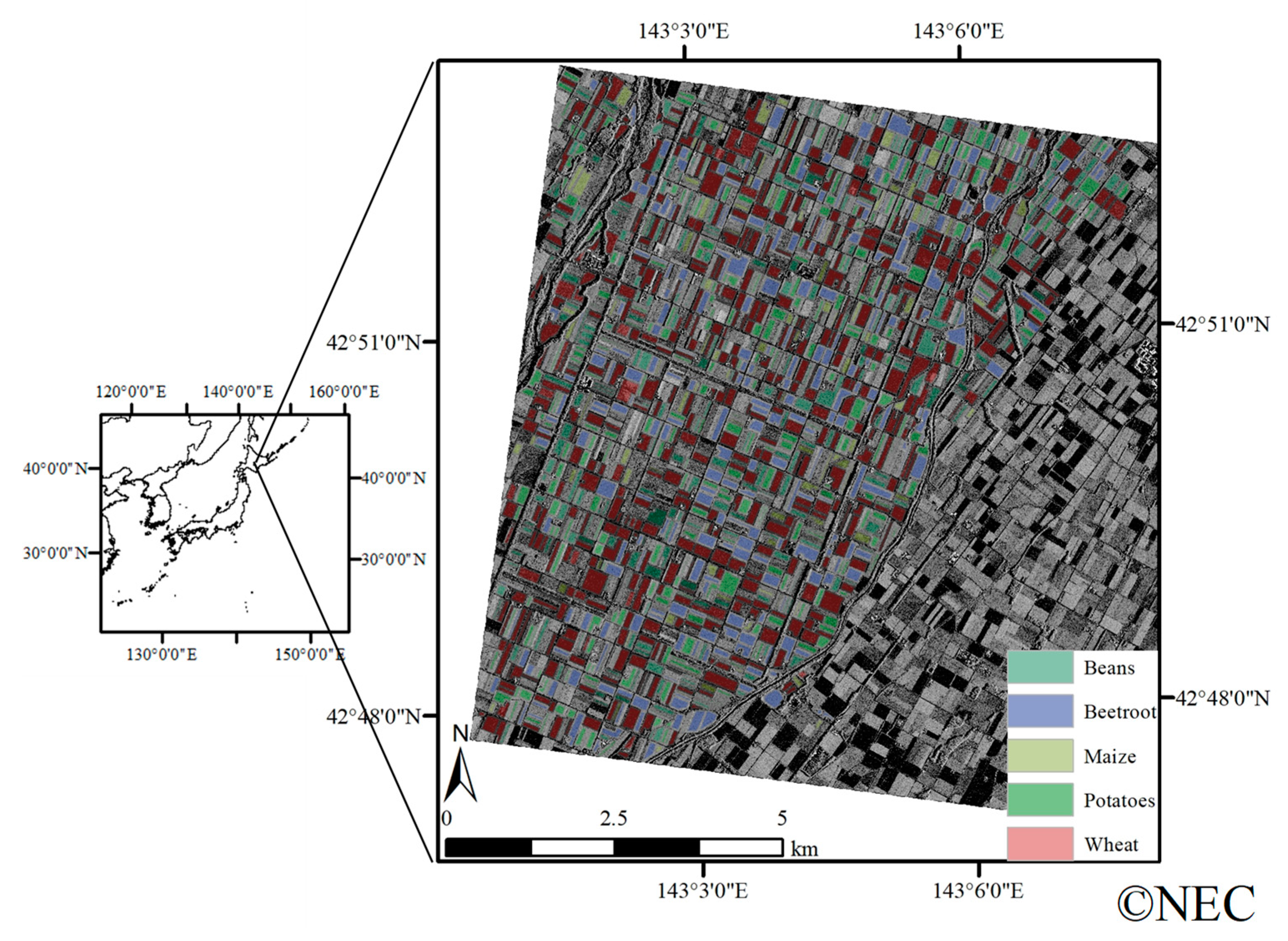
2.1. Study Area
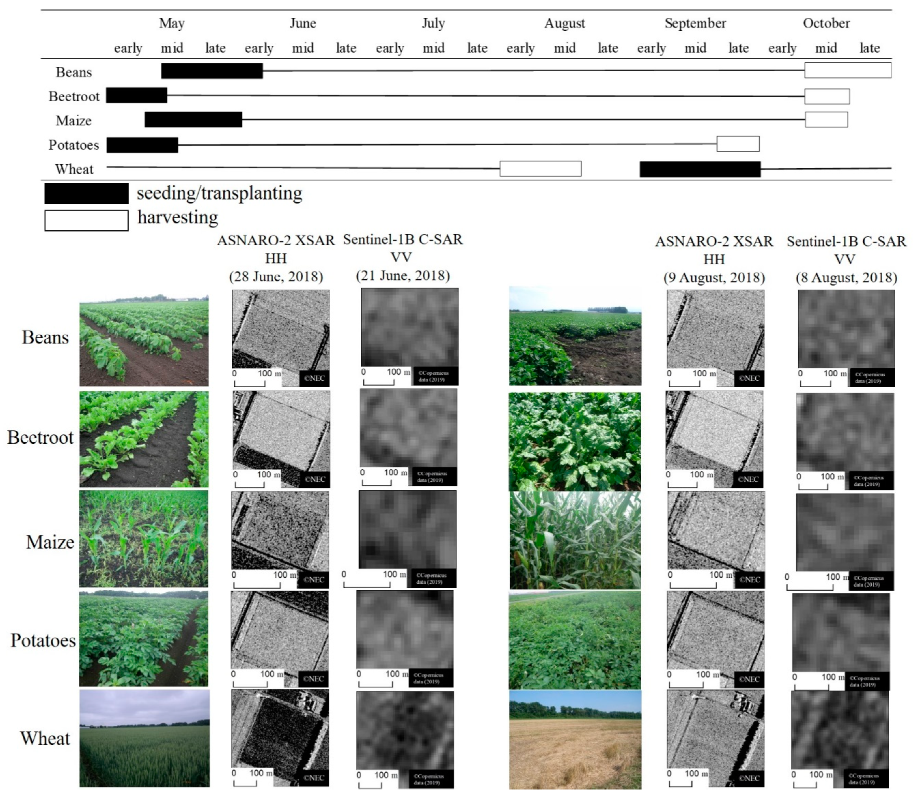
2.2. Reference Data
2.3. Satellite Data
2.4. Classification Procedure
2.5. Accuracy Assessment
3. Results and Discussion
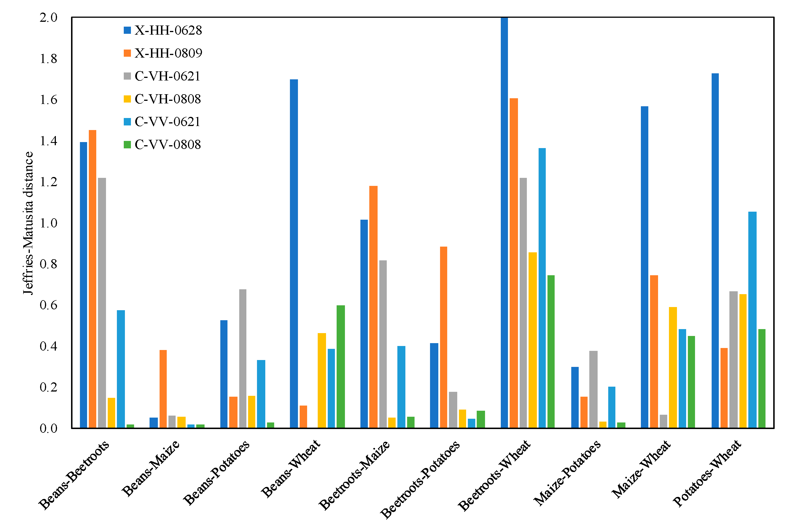
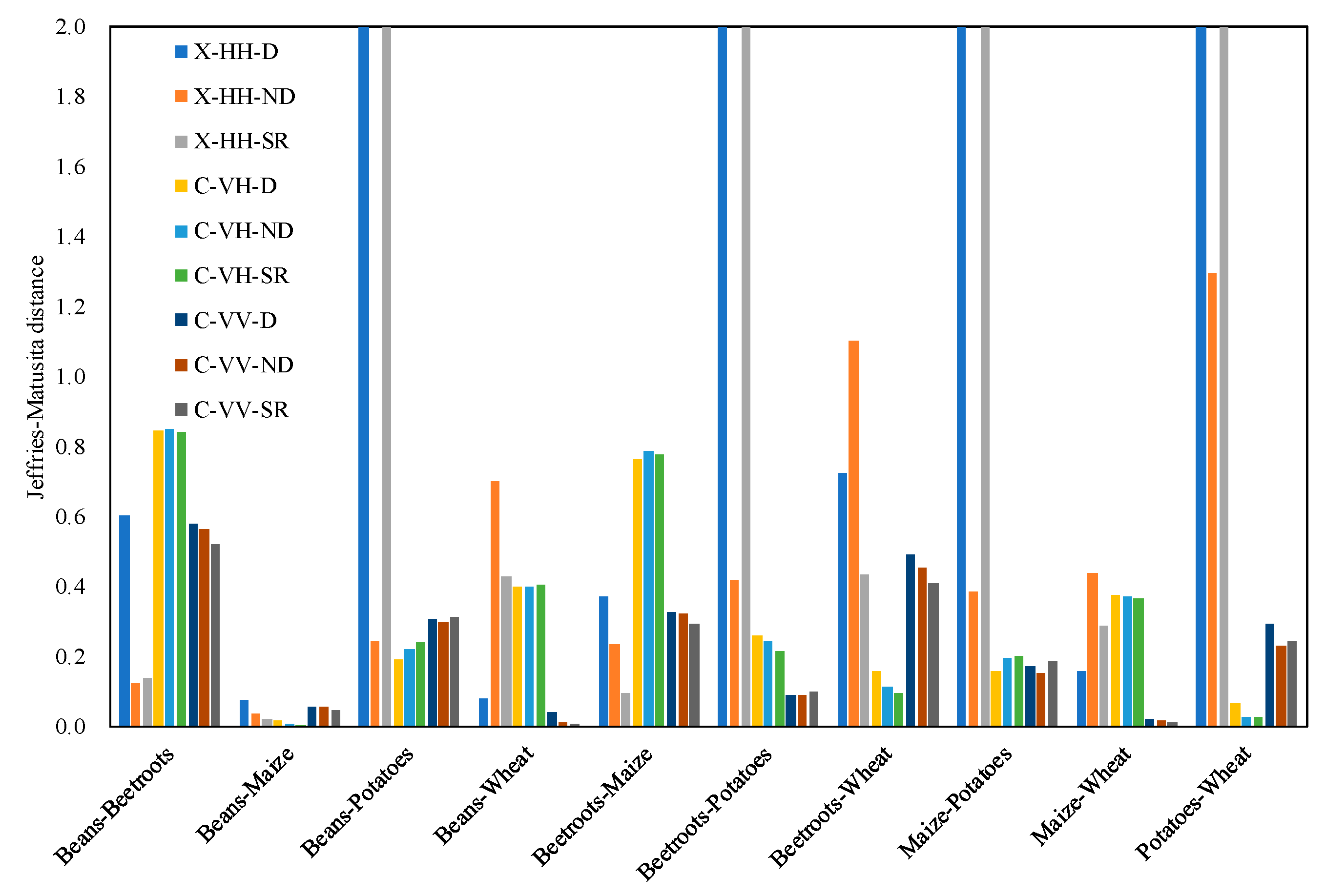
3.1. Separability Assessments
3.2. Accuracy Assessment
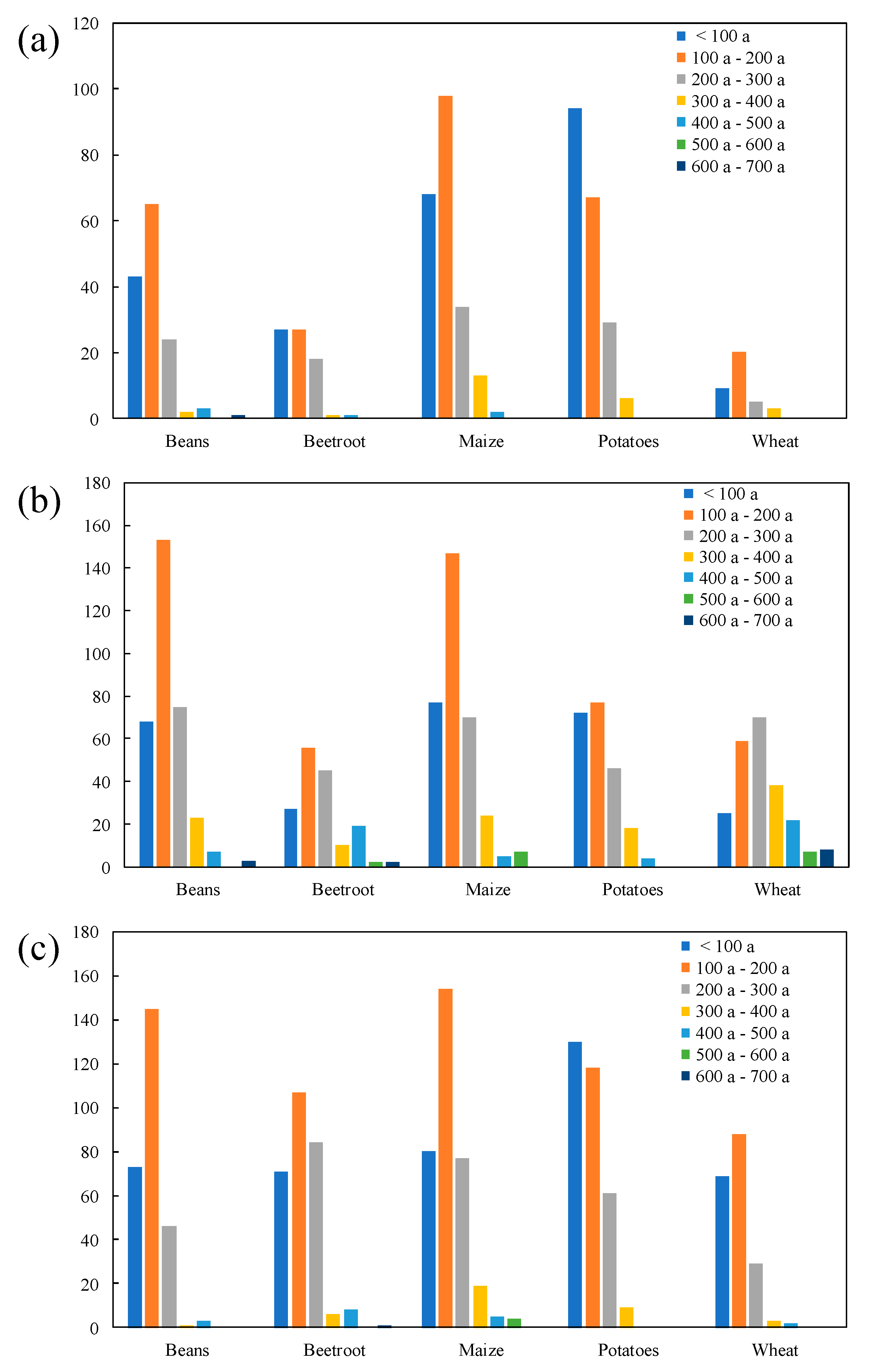
3.3. Misclassified Fields with Respect to Field Area
4. Conclusions
Author Contributions
Funding
Acknowledgments
Conflicts of Interest
References
- Tilman, D.; Cassman, K.G.; Matson, P.A.; Naylor, R.; Polasky, S. Agricultural sustainability and intensive production practices. Nature 2002, 418, 671–677. [Google Scholar] [CrossRef] [PubMed]
- Wardlow, B.D.; Egbert, S.L. Large-area crop mapping using time-series MODIS 250 m NDVI data: An assessment for the U.S. Central Great Plains. Remote Sens. Environ. 2008, 112, 1096–1116. [Google Scholar] [CrossRef]
- Ministry of Agriculture, Forestry and Fisheries. Available online: http://www8.cao.go.jp/space/comittee/dai36/siryou3-5.pdf (accessed on 1 April 2019).
- Sarker, L.R.; Nichol, J.E. Improved forest biomass estimates using ALOS AVNIR-2 texture indices. Remote Sens. Environ. 2011, 115, 968–977. [Google Scholar] [CrossRef]
- Darvishzadeh, R.; Skidmore, A.; Abdullah, H.; Cherenet, E.; Ali, A.; Wang, T.; Nieuwenhuis, W.; Heurich, M.; Vrieling, A.; O’Connor, B.; et al. Mapping leaf chlorophyll content from Sentinel-2 and RapidEye data in spruce stands using the invertible forest reflectance model. Int. J. Appl. Earth Obs. Geoinf. 2019, 79, 58–70. [Google Scholar] [CrossRef]
- Darvishzadeh, R.; Wang, T.; Skidmore, A.; Vrieling, A.; O’Connor, B.; Gara, T.W.; Ens, B.J.; Paganini, M. Analysis of Sentinel-2 and RapidEye for Retrieval of Leaf Area Index in a Saltmarsh Using a Radiative Transfer Model. Remote Sens. 2019, 11, 671. [Google Scholar] [CrossRef]
- Useya, J.; Chen, S.B. Comparative Performance Evaluation of Pixel-Level and Decision-Level Data Fusion of Landsat 8 OLI, Landsat 7 ETM+ and Sentinel-2 MSI for Crop Ensemble Classification. IEEE J. Sel. Top. Appl. Earth Obs. Remote Sens. 2018, 11, 4441–4451. [Google Scholar] [CrossRef]
- Sonobe, R.; Yamaya, Y.; Tani, H.; Wang, X.; Kobayashi, N.; Mochizuki, K.-I. Evaluating metrics derived from Landsat 8 OLI imagery to map crop cover. Geocarto Int. 2018, 34, 839–855. [Google Scholar] [CrossRef]
- Eitel, J.U.H.; Long, D.S.; Gessler, P.E.; Smith, A.M.S. Using in-situ measurements to evaluate the new RapidEye (TM) satellite series for prediction of wheat nitrogen status. Int. J. Remote Sens. 2007, 28, 4183–4190. [Google Scholar] [CrossRef]
- Roy, D.; Wulder, M.; Loveland, T.; Woodcock, C.E.; Allen, R.; Anderson, M.; Helder, D.; Irons, J.; Johnson, D.; Kennedy, R.; et al. Landsat-8: Science and product vision for terrestrial global change research. Remote Sens. Environ. 2014, 145, 154–172. [Google Scholar] [CrossRef]
- Zhang, X.; Wu, B.; Ponce-Campos, G.E.; Zhang, M.; Chang, S.; Tian, F. Mapping up-to-Date Paddy Rice Extent at 10 M Resolution in China through the Integration of Optical and Synthetic Aperture Radar Images. Remote Sens. 2018, 10, 1200. [Google Scholar] [CrossRef]
- Sonobe, R.; Tani, H. Application of the Sahebi model using ALOS/PALSAR and 66.3 cm long surface profile data. Int. J. Remote Sens. 2009, 30, 6069–6074. [Google Scholar] [CrossRef]
- Xu, J.; Li, Z.; Tian, B.; Huang, L.; Chen, Q.; Fu, S. Polarimetric analysis of multi-temporal RADARSAT-2 SAR images for wheat monitoring and mapping. Int. J. Remote Sens. 2014, 35, 3840–3858. [Google Scholar] [CrossRef]
- Sonobe, R.; Tani, H.; Wang, X.; Kobayashi, N.; Shimamura, H. Winter Wheat Growth Monitoring Using Multi-temporal TerraSAR-X Dual-polarimetric Data. Jpn. Agric. Res. Q. JARQ 2014, 48, 471–476. [Google Scholar] [CrossRef]
- Joerg, H.; Pardini, M.; Hajnsek, I.; Papathanassiou, K.P. Sensitivity of SAR Tomography to the Phenological Cycle of Agricultural Crops at X-, C-, and L-band. IEEE J. Sel. Top. Appl. Earth Obs. Remote Sens. 2018, 11, 3014–3029. [Google Scholar] [CrossRef]
- Bouvet, A.; Le Toan, T. Use of ENVISAT/ASAR wide-swath data for timely rice fields mapping in the Mekong River Delta. Remote Sens. Environ. 2011, 115, 1090–1101. [Google Scholar] [CrossRef]
- McNairn, H.; Champagne, C.; Shang, J.; Holmstrom, D.; Reichert, G. Integration of optical and Synthetic Aperture Radar (SAR) imagery for delivering operational annual crop inventories. ISPRS J. Photogramm. Remote Sens. 2009, 64, 434–449. [Google Scholar] [CrossRef]
- Zonno, M.; Bordoni, F.; Matar, J.; de Almeida, F.Q.; Sanjuan-Ferrer, M.J.; Younis, M.; Rodriguez-Cassola, M.; Krieger, G. Sentinel-1 Next Generation: Trade-offs and Assessment of Mission Performance. In Proceedings of the ESA Living Planet Symposium, Milan, Italy, 13–17 May 2019. [Google Scholar]
- Sun, C.; Bian, Y.; Zhou, T.; Pan, J. Using of Multi-Source and Multi-Temporal Remote Sensing Data Improves Crop-Type Mapping in the Subtropical Agriculture Region. Sensors 2019, 19, 2401. [Google Scholar] [CrossRef] [PubMed]
- Mercier, A.; Betbeder, J.; Rumiano, F.; Baudry, J.; Gond, V.; Blanc, L.; Bourgoin, C.; Cornu, G.; Ciudad, C.; Marchamalo, M.; et al. Evaluation of Sentinel-1 and 2 Time Series for Land Cover Classification of Forest–Agriculture Mosaics in Temperate and Tropical Landscapes. Remote Sens. 2019, 11, 979. [Google Scholar] [CrossRef]
- Sonobe, R.; Yamaya, Y.; Tani, H.; Wang, X.; Kobayashi, N.; Mochizuki, K.-I. Assessing the suitability of data from Sentinel-1A and 2A for crop classification. GIScience Remote Sens. 2017, 54, 918–938. [Google Scholar] [CrossRef]
- Stendardi, L.; Karlsen, S.R.; Niedrist, G.; Gerdol, R.; Zebisch, M.; Rossi, M.; Notarnicola, C. Exploiting Time Series of Sentinel-1 and Sentinel-2 Imagery to Detect Meadow Phenology in Mountain Regions. Remote Sens. 2019, 11, 542. [Google Scholar] [CrossRef]
- Clauss, K.; Ottinger, M.; Leinenkugel, P.; Kuenzer, C. Estimating rice production in the Mekong Delta, Vietnam, utilizing time series of Sentinel-1 SAR data. Int. J. Appl. Earth Obs. Geoinf. 2018, 73, 574–585. [Google Scholar] [CrossRef]
- Ndikumana, E.; Minh, D.H.T.; Nguyen, H.D.; Baghdadi, N.; Courault, D.; Hossard, L.; El Moussawi, I. Estimation of Rice Height and Biomass Using Multitemporal SAR Sentinel-1 for Camargue, Southern France. Remote Sens. 2018, 10, 1394. [Google Scholar] [CrossRef]
- Fontanelli, G.; Paloscia, S.; Zribi, M.; Chahbi, A. Sensitivity analysis of X-band SAR to wheat and barley leaf area index in the Merguellil Basin. Remote Sens. Lett. 2013, 4, 1107–1116. [Google Scholar] [CrossRef]
- McNairn, H.; Jiao, X.; Pacheco, A.; Sinha, A.; Tan, W.; Li, Y. Estimating canola phenology using synthetic aperture radar. Remote Sens. Environ. 2018, 219, 196–205. [Google Scholar] [CrossRef]
- Costa, M.P.F. Use of SAR satellites for mapping zonation of vegetation communities in the Amazon floodplain. Int. J. Remote Sens. 2004, 25, 1817–1835. [Google Scholar] [CrossRef]
- National Research and Development Agency and Japan Aerospace Exploration Agency (JAXA). Launch Result, Epsilon-3 with ASNARO-2 Aboard. Available online: https://global.jaxa.jp/press/2018/01/20180118_epsilon3.html (accessed on 5 June 2019).
- Japan EO Satellite Service, Ltd. (JEOSS). Japan EO Satellite Service, Ltd. (JEOSS) Announces the Start of Commercial Operation. Available online: https://jeoss.co.jp/press/japan-eo-satellite-service-ltd-jeoss-announces-the-start-of-commercial-operation/ (accessed on 5 June 2019).
- Sonobe, R. Parcel-Based Crop Classification Using Multi-Temporal TerraSAR-X Dual Polarimetric Data. Remote Sens. 2019, 11, 1148. [Google Scholar] [CrossRef]
- Burges, C.J. A Tutorial on Support Vector Machines for Pattern Recognition. Data Min. Knowl. Discov. 1998, 2, 121–167. [Google Scholar] [CrossRef]
- Foody, G.; Mathur, A. A relative evaluation of multiclass image classification by support vector machines. IEEE Trans. Geosci. Remote Sens. 2004, 42, 1335–1343. [Google Scholar] [CrossRef]
- Sonobe, R.; Tani, H.; Wang, X.; Kobayashi, N.; Shimamura, H. Discrimination of crop types with TerraSAR-X-derived information. Phys. Chem. Earth Parts A B C 2015, 2–13. [Google Scholar] [CrossRef]
- Biau, G.; Scornet, E. A random forest guided tour. TEST 2016, 25, 197–227. [Google Scholar] [CrossRef]
- Sonobe, R.; Sano, T.; Horie, H. Using spectral reflectance to estimate leaf chlorophyll content of tea with shading treatments. Biosyst. Eng. 2018, 175, 168–182. [Google Scholar] [CrossRef]
- Pal, M. Random forest classifier for remote sensing classification. Int. J. Remote Sens. 2005, 26, 217–222. [Google Scholar] [CrossRef]
- Pal, M.; Maxwell, A.E.; Warner, T.A. Kernel-based extreme learning machine for remote-sensing image classification. Remote Sens. Lett. 2013, 4, 853–862. [Google Scholar] [CrossRef]
- Sonobe, R.; Tani, H.; Wang, X.F. An experimental comparison between KELM and CART for crop classification using Landsat-8 OLI data. Geocarto Int. 2017, 32, 128–138. [Google Scholar] [CrossRef]
- Cooner, A.J.; Shao, Y.; Campbell, J.B. Detection of Urban Damage Using Remote Sensing and Machine Learning Algorithms: Revisiting the 2010 Haiti Earthquake. Remote Sens. 2016, 8, 868. [Google Scholar] [CrossRef]
- Puertas, O.L.; Brenning, A.; Meza, F.J. Balancing misclassification errors of land cover classification maps using support vector machines and Landsat imagery in the Maipo river basin (Central Chile, 1975–2010). Remote Sens. Environ. 2013, 137, 112–123. [Google Scholar] [CrossRef]
- Bergstra, J.; Bengio, Y. Random Search for Hyper-Parameter Optimization. J. Mach. Learn. Res. 2012, 13, 281–305. [Google Scholar]
- Monsivais-Huertero, A.; Liu, P.W.; Judge, J. Phenology-Based Backscattering Model for Corn at L-Band. IEEE Trans. Geosci. Remote Sens. 2018, 56, 4989–5005. [Google Scholar] [CrossRef]
- Shoshany, M.; Svoray, T.; Curran, P.J.; Foody, G.M.; Perevolotsky, A. The relationship between ERS-2 SAR backscatter and soil moisture: Generalization from a humid to semi-arid transect. Int. J. Remote Sens. 2000, 21, 2337–2343. [Google Scholar] [CrossRef]
- Betbeder, J.; Fieuzal, R.; Philippets, Y.; Ferro-Famil, L.; Baup, F. Contribution of multitemporal polarimetric synthetic aperture radar data for monitoring winter wheat and rapeseed crops. J. Appl. Remote Sens. 2016, 10, 026020. [Google Scholar] [CrossRef]
- Kim, Y.; Jackson, T.; Bindlish, R.; Lee, H.; Hong, S. Radar Vegetation Index for Estimating the Vegetation Water Content of Rice and Soybean. IEEE Geosci. Remote Sens. Lett. 2012, 9, 564–568. [Google Scholar]
- Richards, J.A. Remote Sensing Digital Image Analysis; Springer: Berlin/Heidelberg, Germany, 2013. [Google Scholar]
- Hastie, T.; Tibshirani, R.; Friedman, J. The Elements of Statistical Learning: Data Mining, Inference, and Prediction, 2nd ed.; Springer: New York, NY, USA, 2009; p. 745. [Google Scholar]
- R Core Team. R: A Language and Environment for Statistical Computing. Available online: https://www.R-project.org/ (accessed on 5 June 2019).
- Cortes, C.; Vapnik, V. Support-Vector Networks. Mach. Learn. 1995, 20, 273–297. [Google Scholar] [CrossRef]
- Aizerman, M.; Braverman, E.; Rozonoer, L. Theoretical foundations of the potential function method in pattern recognition learning. Autom. Remote Control 1964, 25, 821–837. [Google Scholar]
- Melgani, F.; Bruzzone, L. Classification of hyperspectral remote sensing images with support vector machines. IEEE Trans. Geosci. Remote Sens. 2004, 42, 1778–1790. [Google Scholar] [CrossRef]
- Camps-Valls, G.; Bruzzone, L. Kernel-based methods for hyperspectral image classification. IEEE Trans. Geosci. Remote Sens. 2005, 43, 1351–1362. [Google Scholar] [CrossRef]
- Kavzoglu, T.; Colkesen, I. A kernel functions analysis for support vector machines for land cover classification. Int. J. Appl. Earth Obs. Geoinf. 2009, 11, 352–359. [Google Scholar] [CrossRef]
- Breiman, L. Random forests. Mach. Learn. 2001, 45, 5–32. [Google Scholar] [CrossRef]
- Liaw, A.; Wiener, M. Classification and regression by random Forest. R News 2002, 2, 18–22. [Google Scholar]
- Ishwaran, H.; Kogalur, U.B. Random survival forests for R. R News 2007, 7, 25–31. [Google Scholar]
- Ishwaran, H.; Kogalur, U.B.; Blackstone, E.H.; Lauer, M.S. Random survival forests. Ann. Appl. Stat. 2008, 2, 841–860. [Google Scholar] [CrossRef]
- Sonobe, R.; Yamaya, Y.; Tani, H.; Wang, X.; Kobayashi, N.; Mochizuki, K.I. Mapping crop cover using multi-temporal Landsat 8 OLI imagery. Int. J. Remote Sens. 2017, 38, 4348–4361. [Google Scholar] [CrossRef]
- Svozil, D.; Kvasnička, V.; Pospichal, J. Introduction to multi-layer feed-forward neural networks. Chemom. Intell. Lab. Syst. 1997, 39, 43–62. [Google Scholar] [CrossRef]
- Srivastava, N.; Hinton, G.; Krizhevsky, A.; Sutskever, I.; Salakhutdinov, R. Dropout: A Simple Way to Prevent Neural Networks from Overfitting. J. Mach. Learn. Res. 2014, 15, 1929–1958. [Google Scholar]
- Pontius, R.G.; Millones, M. Death to Kappa: Birth of quantity disagreement and allocation disagreement for accuracy assessment. Int. J. Remote Sens. 2011, 32, 4407–4429. [Google Scholar] [CrossRef]
- McNemar, Q. Note on the sampling error of the difference between correlated proportions or percentages. Psychometrika 1947, 12, 153–157. [Google Scholar] [CrossRef]
- Macelloni, G.; Paloscia, S.; Pampaloni, P.; Marliani, F.; Gai, M. The relationship between the backscattering coefficient and the biomass of narrow and broad leaf crops. IEEE Trans. Geosci. Remote Sens. 2002, 39, 873–884. [Google Scholar] [CrossRef]
- Baker, B.A.; Warner, T.A.; Conley, J.F.; McNeil, B.E. Does spatial resolution matter? A multi-scale comparison of object-based and pixel-based methods for detecting change associated with gas well drilling operations. Int. J. Remote Sens. 2013, 34, 1633–1651. [Google Scholar] [CrossRef]
- Lv, T.T.; Liu, C. Study on extraction of crop information using time-series MODIS data in the Chao Phraya Basin of Thailand. Adv. Space Res. 2010, 45, 775–784. [Google Scholar] [CrossRef]
- Avci, Z.D.U.; Sunar, F. Process-based image analysis for agricultural mapping: A case study in Turkgeldi region, Turkey. Adv. Space Res. 2015, 56, 1635–1644. [Google Scholar] [CrossRef]
- Guarini, R.; Bruzzone, L.; Santoni, M.; Dini, L. Analysis on the Effectiveness of Multi-Temporal COSMO-SkyMed Images for Crop Classification. In Proceedings of the Conference on Image and Signal Processing for Remote Sensing XXI, Toulouse, France, 21–23 September 2015. [Google Scholar]
- Goodin, D.G.; Anibas, K.L.; Bezymennyi, M. Mapping land cover and land use from object-based classification: An example from a complex agricultural landscape. Int. J. Remote Sens. 2015, 36, 4702–4723. [Google Scholar] [CrossRef]
- Azar, R. Assessing in-season crop classification performance using satellite data: A test case in Northern Italy. Eur. J. Remote Sens. 2016, 49, 361–380. [Google Scholar] [CrossRef]
- Kussul, N.; Lemoine, G.; Gallego, F.J.; Skakun, S.V.; Lavreniuk, M.; Shelestov, A.Y. Parcel-Based Crop Classification in Ukraine Using Landsat-8 Data and Sentinel-1A Data. IEEE J. Sel. Top. Appl. Earth Obs. Remote Sens. 2016, 9, 2500–2508. [Google Scholar] [CrossRef]
- Gao, Q.; Zribi, M.; Escorihuela, M.J.; Baghdadi, N.; Segui, P.Q. Irrigation Mapping Using Sentinel-1 Time Series at Field Scale. Remote Sens. 2018, 10, 1495. [Google Scholar] [CrossRef]
- Amazirh, A.; Merlin, O.; Er-Raki, S.; Gao, Q.; Rivalland, V.; Malbeteau, Y.; Khabba, S.; Escorihuela, M.J. Retrieving surface soil moisture at high spatio-temporal resolution from a synergy between Sentinel-1 radar and Landsat thermal data: A study case over bare soil. Remote Sens. Environ. 2018, 211, 321–337. [Google Scholar] [CrossRef]


| Satellite/Sensor | Acquisition Date | Mode | Polarization | Off Nadir Angle (°) | Incidence Angle (°) | Pass Direction | Look Direction | |
|---|---|---|---|---|---|---|---|---|
| Near | Far | |||||||
| Sentinel-1B C-SAR | 21 June 2018 | IW | VH/VV | 30.61 | 45.88 | Ascending | Right | |
| ASNARO-2/XSAR | 28 June 2018 | Spotlight | HH | 42.49 | Descending | Right | ||
| Sentinel-1B C-SAR | 08 August 2018 | IW | VH/VV | 30.61 | 45.88 | Ascending | Right | |
| ASNARO-2/XSAR | 09 August 2018 | Spotlight | HH | 42.50 | Descending | Right | ||
| Training Data | Validation Data | Test Data | |
|---|---|---|---|
| Beans | 183 | 92 | 92 |
| Beetroots | 155 | 77 | 78 |
| Maize | 74 | 37 | 37 |
| Potatoes | 225 | 113 | 113 |
| Wheat | 264 | 132 | 133 |
| SVM | RF | KELM | FNN | |||||||||
|---|---|---|---|---|---|---|---|---|---|---|---|---|
| Case 1 | Case 2 | Case 3 | Case 1 | Case 2 | Case 3 | Case 1 | Case 2 | Case 3 | Case 1 | Case 2 | Case 3 | |
| PA | ||||||||||||
| Beans | 0.850 ± 0.022 | 0.639 ± 0.102 | 0.709 ± 0.048 | 0.807 ± 0.037 | 0.672 ± 0.037 | 0.705 ± 0.043 | 0.817 ± 0.041 | 0.682 ± 0.074 | 0.683 ± 0.032 | 0.813 ± 0.060 | 0.583 ± 0.104 | 0.660 ± 0.088 |
| Beetroots | 0.905 ± 0.042 | 0.786 ± 0.223 | 0.645 ± 0.050 | 0.909 ± 0.032 | 0.914 ± 0.033 | 0.633 ± 0.053 | 0.881 ± 0.047 | 0.836 ± 0.186 | 0.677 ± 0.060 | 0.899 ± 0.036 | 0.935 ± 0.029 | 0.687 ± 0.062 |
| Maize | 0.414 ± 0.065 | 0.114 ± 0.102 | 0.078 ± 0.078 | 0.300 ± 0.091 | 0.281 ± 0.082 | 0.084 ± 0.048 | 0.230 ± 0.126 | 0.035 ± 0.085 | 0.041 ± 0.045 | 0.408 ± 0.119 | 0.327 ± 0.099 | 0.157 ± 0.071 |
| Potatoes | 0.827 ± 0.035 | 0.810 ± 0.068 | 0.719 ± 0.040 | 0.854 ± 0.034 | 0.795 ± 0.031 | 0.699 ± 0.045 | 0.806 ± 0.050 | 0.619 ± 0.060 | 0.687 ± 0.044 | 0.826 ± 0.057 | 0.788 ± 0.055 | 0.689 ± 0.050 |
| Wheat | 0.972 ± 0.024 | 0.824 ± 0.343 | 0.855 ± 0.029 | 0.978 ± 0.013 | 0.970 ± 0.021 | 0.856 ± 0.031 | 0.980 ± 0.016 | 0.929 ± 0.109 | 0.874 ± 0.028 | 0.980 ± 0.013 | 0.977 ± 0.011 | 0.849 ± 0.028 |
| UA | ||||||||||||
| Beans | 0.787 ± 0.036 | 0.669 ± 0.069 | 0.639 ± 0.045 | 0.770 ± 0.053 | 0.694 ± 0.047 | 0.628 ± 0.054 | 0.745 ± 0.025 | 0.504 ± 0.086 | 0.651 ± 0.043 | 0.796 ± 0.049 | 0.723 ± 0.059 | 0.656 ± 0.061 |
| Beetroots | 0.874 ± 0.037 | 0.882 ± 0.043 | 0.702 ± 0.041 | 0.892 ± 0.033 | 0.879 ± 0.033 | 0.679 ± 0.043 | 0.852 ± 0.053 | 0.829 ± 0.051 | 0.684 ± 0.032 | 0.873 ± 0.047 | 0.855 ± 0.038 | 0.673 ± 0.050 |
| Maize | 0.713 ± 0.091 | 0.704 ± 0.214 | 0.301 ± 0.201 | 0.650 ± 0.128 | 0.595 ± 0.100 | 0.508 ± 0.209 | 0.718 ± 0.176 | 0.187 ± 0.291 | 0.679 ± 0.322 | 0.687 ± 0.123 | 0.570 ± 0.154 | 0.413 ± 0.119 |
| Potatoes | 0.800 ± 0.020 | 0.609 ± 0.157 | 0.640 ± 0.027 | 0.780 ± 0.021 | 0.688 ± 0.016 | 0.623 ± 0.024 | 0.770 ± 0.033 | 0.687 ± 0.060 | 0.615 ± 0.031 | 0.791 ± 0.024 | 0.678 ± 0.026 | 0.642 ± 0.044 |
| Wheat | 0.964 ± 0.015 | 0.950 ± 0.023 | 0.788 ± 0.030 | 0.958 ± 0.017 | 0.961 ± 0.018 | 0.794 ± 0.024 | 0.937 ± 0.018 | 0.920 ± 0.034 | 0.777 ± 0.031 | 0.951 ± 0.017 | 0.944 ± 0.027 | 0.799 ± 0.032 |
| F1 | ||||||||||||
| Beans | 0.817 ± 0.022 | 0.645 ± 0.051 | 0.671 ± 0.033 | 0.787 ± 0.034 | 0.682 ± 0.034 | 0.664 ± 0.041 | 0.779 ± 0.024 | 0.574 ± 0.066 | 0.666 ± 0.030 | 0.802 ± 0.030 | 0.637 ± 0.057 | 0.652 ± 0.041 |
| Beetroots | 0.889 ± 0.036 | 0.810 ± 0.157 | 0.672 ± 0.040 | 0.900 ± 0.025 | 0.896 ± 0.026 | 0.655 ± 0.044 | 0.866 ± 0.044 | 0.817 ± 0.101 | 0.680 ± 0.039 | 0.885 ± 0.031 | 0.893 ± 0.025 | 0.677 ± 0.031 |
| Maize | 0.519 ± 0.062 | 0.218 ± 0.122 | 0.169 ± 0.090 | 0.406 ± 0.101 | 0.375 ± 0.080 | 0.142 ± 0.079 | 0.320 ± 0.143 | 0.153 ± 0.161 | 0.100 ± 0.067 | 0.496 ± 0.102 | 0.397 ± 0.081 | 0.214 ± 0.082 |
| Potatoes | 0.813 ± 0.025 | 0.676 ± 0.112 | 0.676 ± 0.027 | 0.815 ± 0.023 | 0.737 ± 0.018 | 0.658 ± 0.028 | 0.786 ± 0.030 | 0.649 ± 0.044 | 0.649 ± 0.033 | 0.807 ± 0.036 | 0.728 ± 0.025 | 0.663 ± 0.025 |
| Wheat | 0.968 ± 0.010 | 0.918 ± 0.131 | 0.820 ± 0.026 | 0.968 ± 0.007 | 0.965 ± 0.010 | 0.823 ± 0.022 | 0.957 ± 0.008 | 0.920 ± 0.055 | 0.822 ± 0.022 | 0.965 ± 0.009 | 0.960 ± 0.010 | 0.823 ± 0.025 |
| OA | 0.854 ± 0.018 | 0.712 ± 0.072 | 0.692 ± 0.015 | 0.845 ± 0.017 | 0.800 ± 0.014 | 0.685 ± 0.019 | 0.825 ± 0.023 | 0.712 ± 0.072 | 0.687 ± 0.016 | 0.847 ± 0.021 | 0.789 ± 0.016 | 0.686 ± 0.018 |
| Kappa | 0.810 ± 0.023 | 0.626 ± 0.090 | 0.595 ± 0.020 | 0.798 ± 0.022 | 0.739 ± 0.019 | 0.586 ± 0.025 | 0.772 ± 0.030 | 0.626 ± 0.090 | 0.588 ± 0.021 | 0.801 ± 0.027 | 0.726 ± 0.020 | 0.590 ± 0.023 |
| AD | 0.107 ± 0.018 | 0.130 ± 0.042 | 0.228 ± 0.024 | 0.105 ± 0.021 | 0.145 ± 0.021 | 0.234 ± 0.018 | 0.116 ± 0.022 | 0.166 ± 0.050 | 0.230 ± 0.014 | 0.111 ± 0.028 | 0.139 ± 0.028 | 0.238 ± 0.013 |
| QD | 0.039 ± 0.008 | 0.152 ± 0.186 | 0.080 ± 0.013 | 0.050 ± 0.009 | 0.056 ± 0.012 | 0.081 ± 0.008 | 0.059 ± 0.012 | 0.122 ± 0.048 | 0.084 ± 0.009 | 0.042 ± 0.014 | 0.071 ± 0.027 | 0.076 ± 0.012 |
| AD + QD | 0.146 ± 0.018 | 0.282 ± 0.147 | 0.308 ± 0.015 | 0.155 ± 0.017 | 0.200 ± 0.014 | 0.315 ± 0.019 | 0.175 ± 0.023 | 0.288 ± 0.072 | 0.313 ± 0.016 | 0.153 ± 0.021 | 0.211 ± 0.016 | 0.314 ± 0.018 |
| SVM | RF | KELM | FNN | |||||||||
|---|---|---|---|---|---|---|---|---|---|---|---|---|
| Case 2 | Case 3 | Case 1 | Case 2 | Case 3 | Case 1 | Case 2 | Case 3 | Case 1 | Case 2 | Case 3 | ||
| SVM | Case 1 | 17.42 + 7.37 | 21.35 + 5.08 | 12.08 + 4.11 | 12.89 + 6.55 | 22.82 + 7.58 | 20.89 + 4.81 | 41.24 + 23.45 | 28.7 + 8.71 | 14.53 + 6 | 27.65 + 17.81 | 19 + 7.81 |
| Case 2 | 17.45 + 8.09 | 17.51 + 5.88 | 19.68 + 7.89 | 14.13 + 4.31 | 15.69 + 3.92 | 32.84 + 15.36 | 15.31 + 6 | 22.84 + 9.77 | 32.61 + 14.45 | 20.45 + 8.15 | ||
| Case 3 | 16.34 + 5.81 | 23.05 + 5.54 | 11.77 + 3.15 | 16.94 + 8.17 | 32.61 + 25.22 | 24.8 + 9.4 | 22.49 + 7.11 | 30.83 + 9.58 | 31.31 + 12.39 | |||
| RF | Case 1 | 10.49 + 5.54 | 16.1 + 6.21 | 21.15 + 7.55 | 45.77 + 29.22 | 23.25 + 8.4 | 14.02 + 4.51 | 28.24 + 13.94 | 13.5 + 5.99 | |||
| Case 2 | 22.37 + 6.66 | 22.24 + 8.21 | 53.89 + 27.19 | 25.71 + 9.95 | 14.33 + 6.27 | 25.59 + 18.25 | 18.65 + 7.66 | |||||
| Case 3 | 17.79 + 8.1 | 32.17 + 25.89 | 19.38 + 6.03 | 23.76 + 7.69 | 31.87 + 13.09 | 26.96 + 11.41 | ||||||
| KELM | Case 1 | 36.75 + 26.05 | 23.23 + 12.43 | 26.93 + 10.16 | 32.95 + 18.04 | 24.58 + 12.1 | ||||||
| Case 2 | 25.62 + 13.34 | 38.78 + 17.12 | 52.53 + 16.47 | 27.31 + 15.94 | ||||||||
| Case 3 | 28.03 + 11.36 | 31.82 + 13.86 | 33.36 + 13.74 | |||||||||
| FNN | Case 1 | 25.95 + 12.73 | 18.44 + 8.89 | |||||||||
| Case 2 | 22.96 + 10.57 | |||||||||||
| Sensor | Algorithm | Study Area | Class | Overall Accuracy | Reference |
|---|---|---|---|---|---|
| CBERS-02B | Support vector machine | Chao Phraya Basin, Thailand | paddy fields, field crops, forest, water | 0.7996 | [65] |
| SPOT 4 | Decision-based process | Marmara, Turkey | flamura, guadalupe, pehlivan, vetch, sunflower, corn I, corn II, clover, river, urban, mixed | 0.80 | [66] |
| COSMO-SkyMed | Support vector machine | Lower Austria | carrot, corn, potato, soybean, sugar beet | 0.845 | [67] |
| Landsat-8 OLI | Support vector machine | Ukraine–Poland border | artificial/urban, bare, grassland or herbaceous cover, woodland, wetland, water | 0.89 | [68] |
| Landsat-8 OLI | Maximum likelihood | Northern Italy | maize, rice, soybean, winter crops, forage crops | 0.927 | [69] |
| Landsat-8 OLI, Sentinel-1 | Neural networks | North of Ukraine | winter wheat, winter rapeseed, maize, sugar beet, sunflower, soybean | 0.894 | [70] |
| Sentinel-1, Sentinel-2, and Landsat-8 | Random Forest | The lower reaches of the Yangzi River in China | forest, maize, rape, urban, water, wheat | 0.93 | [19] |
© 2019 by the author. Licensee MDPI, Basel, Switzerland. This article is an open access article distributed under the terms and conditions of the Creative Commons Attribution (CC BY) license (http://creativecommons.org/licenses/by/4.0/).
Share and Cite
Sonobe, R. Combining ASNARO-2 XSAR HH and Sentinel-1 C-SAR VH/VV Polarization Data for Improved Crop Mapping. Remote Sens. 2019, 11, 1920. https://doi.org/10.3390/rs11161920
Sonobe R. Combining ASNARO-2 XSAR HH and Sentinel-1 C-SAR VH/VV Polarization Data for Improved Crop Mapping. Remote Sensing. 2019; 11(16):1920. https://doi.org/10.3390/rs11161920
Chicago/Turabian StyleSonobe, Rei. 2019. "Combining ASNARO-2 XSAR HH and Sentinel-1 C-SAR VH/VV Polarization Data for Improved Crop Mapping" Remote Sensing 11, no. 16: 1920. https://doi.org/10.3390/rs11161920
APA StyleSonobe, R. (2019). Combining ASNARO-2 XSAR HH and Sentinel-1 C-SAR VH/VV Polarization Data for Improved Crop Mapping. Remote Sensing, 11(16), 1920. https://doi.org/10.3390/rs11161920