An Accurate Visual-Inertial Integrated Geo-Tagging Method for Crowdsourcing-Based Indoor Localization

Abstract

One of the unavoidable bottlenecks in the public application of passive signal (e.g., received signal strength, magnetic) fingerprinting-based indoor localization technologies is the extensive human effort that is required to construct and update database for indoor positioning. In this paper, we propose an accurate visual-inertial integrated geo-tagging method that can be used to collect fingerprints and construct the radio map by exploiting the crowdsourced trajectory of smartphone users. By integrating multisource information from the smartphone sensors (e.g., camera, accelerometer, and gyroscope), this system can accurately reconstruct the geometry of trajectories. An algorithm is proposed to estimate the spatial location of trajectories in the reference coordinate system and construct the radio map and geo-tagged image database for indoor positioning. With the help of several initial reference points, this algorithm can be implemented in an unknown indoor environment without any prior knowledge of the floorplan or the initial location of crowdsourced trajectories. The experimental results show that the average calibration error of the fingerprints is 0.67 m. A weighted k-nearest neighbor method (without any optimization) and the image matching method are used to evaluate the performance of constructed multisource database. The average localization error of received signal strength (RSS) based indoor positioning and image based positioning are 3.2 m and 1.2 m, respectively, showing that the quality of the constructed indoor radio map is at the same level as those that were constructed by site surveying. Compared with the traditional site survey based positioning cost, this system can greatly reduce the human labor cost, with the least external information.

1. Introduction

Nowadays, indoor localization has become a common issue for various location-based services and applications. A number of technologies have been proposed for indoor localization, which are based on different principles, such as Wi-Fi [1], geomagnetic [2], ultra wide band (UWB) [3], ultrasound [4] and so on. Among these localization technologies, ultrasound and UWB can be used to estimate the distance between the source and terminals, which can provide accurate localization results. However, such technologies require an extra deployment of localization devices, which restricts their large-scale applications. Many studies have focused on developing localization scheme that do not rely on extra devices or only use the existing infrastructures, such as Wi-Fi fingerprinting [5,6,7,8], geomagnetic [9], or visual positioning [10,11,12]. For example, crowd participants walking in the indoor environment can collect the fingerprints and construct radio map or magnetic map by uploading their inertial data, Wi-Fi received signal strength (RSS) data or magnetic readings, which can be directly used for indoor localization. For image matching-based visual positioning, pictures that are taken by a user can be matched against the geo-tagged images stored in a database. The location of a geo-tagged image can be used as the localization results when the two images (the query image and the geo-tagged image) are successfully matched with each other.

The collection of data is an essential bottleneck for developing localization solutions with free of additional devices. For example, Wi-Fi fingerprinting-based localization requires a radio map of the whole environment. Visual-based positioning relies on the image database or other semantic information to represent locations. Geomagnetic-based localization depends on a similar map of magnetic field strength of the environment. The collection and updating of the required data are quite labor-intensive and time-consuming which hinders these localization solutions from large-scale application. To solve this issue, many studies propose the use of crowdsourcing-based approaches to reduce the labor and time cost that needed for data collection [13,14,15,16,17,18,19,20,21,22]. For example, it has been exploited that smartphones collect RSS and inertial data to construct radio map with unconscious cooperation among volunteers [19,20,21]. These methods can construct the fingerprint database effectively with less time consuming. However, most of these methods still require user intervention [16] or prior knowledge e.g., initial radio map [21,23], access point’s (AP) location [22], initial location of volunteers [21], or indoor floorplans [13,16,17,18]. In practice, it is usually difficult to collect all of the required data, such as the method proposed in [23] uses image matching to improve the localization accuracy of Wi-Fi fingerprinting. However, it requires an initial Wi-Fi radio map as an initial input, which is suitable for the updating Wi-Fi database. GROPING [24] is a self-contained indoor navigation system that relies on geomagnetic fingerprinting. It exploits crowdsensing walking trajectories to construct floor maps and semantic navigation map while using user contributed sensor data and semantic labels. However, although visual positioning can achieve good positioning accuracy and it does not rely on extra infrastructure, the study of crowdsourcing-based visual positioning is much fewer than that of Wi-Fi and magnetic positioning. The existing studies [11,25,26] mainly concentrate on developing new algorithm or model to improve the accuracy of visual positioning. Less attention has been devoted to developing an efficient and reliable indoor image collection and geo-tagging method. The lack of a large mount of indoor geo-tagged image databases is an essential bottleneck in the application of visual positioning. If a crowdsourcing-based image collection and geo-tagging method can be proposed, the difficulty for deploying visual positioning systems or services may be significantly reduced.

As a wide-spread mobile device, the smartphone is suitable for collecting crowdsourcing data, including wireless signals, inertial data, magnetic field, image, and so on. While people are walking in different indoor environments, their smartphones can collect the required data continuously at a certain sampling rate. The collected signals are associated with the corresponding sampling points with timestamps. However, the spatial location of sampling points cannot be directly received from smartphone built-in sensors in indoor spaces. The geo-tagging of trajectory sampling points is a key issue for crowdsourcing-based localization approaches. The intervention of users has been considered in some studies to facilitate the geo-tagging of trajectory. For example, Redpin [27] and OIL [28] prompt the users to recognize their current location for trajectory tracking based on a prior build-in displayed map. Without initial indoor map, Elekspot [29] and FreeLoc [16] take the advantage of the semantic labels that are associated with a trajectory, such as room or corridor. Consequently, the localization result of these methods is at a semantic level. Instead of user intervention, other studies realize trajectory geo-tagging by using smartphone sensors and the map matching method. For example, RCILS [13], LiFS [17], Zee [18], and WILL [30] used the pedestrian dead-reckoning (PDR) method to recover the trajectory of smartphone users. The recovered trajectory can be spatially matched to an indoor floor plan by using an activity recognition mechanism. However, this map matching mechanism highly depends on an assumption that all activities of a user occur at the special locations in an indoor space (e.g., intersections or corners). This assumption is vulnerable to the randomness of human activity. For example, if one person makes a free turn not at a special location, this method may match this activity to an incorrect location. Much effort has been made to improve the performance of trajectory estimation [31,32,33,34]. For example, the trajectory alignment and calibration method proposed in [32] can align a crowdsourcing trajectory into a coordinate system by using a foot-mounted inertial sensor and Wi-Fi RSS measurements. CrowdMap [33] jointly leverage crowdsourced sensor data and video data to track the movements of users. It takes the latest known GPS position as an initial location and the user can modify it if it is incorrect. The video frames can be used to improve the localization accuracy. Pan et al. [34] provides a collaborative filtering with graph-based semi-supervised learning method to estimate the location of user, as well as the location of APs. A training phase is needed to calibrate a probabilistic location estimation system. In summary, although progress has been made in pedestrian tracking and trajectory estimation, but the requirement of extra devices, user intervention, or prior knowledge limits the practical use of these approaches. It remains a question as to how to improve the accuracy and robustness of smartphone-based geo-tagging with least device or prior knowledge requirements.

Another problem is the diversity of smartphone devices. The collected wireless signal probably will be different for two smartphone devices even at a same spatial location due to the difference of built-in sensors in smartphone. It will obviously affect the geo-tagging accuracy of the Wi-Fi or geomagnetic clustering based crowdsourcing methods. However, it is difficult to meet the condition, where all crowdsourcing users have the same type of smartphone devices. Some studies have tried to solve this problem by calibrating RSS fingerprints that were collected by different devices. For example, in [29], a calibration matrix has been constructed for all supported devices. The elements from the matrix represent the linear regression relation between different devices. In [35], the diversity of devices and its effect on localization have been analyzed. A kernel function has been proposed to model the distribution of RSS. It applies local variations as a compensation for linear transformation between two devices. However, the accurately calibration of Wi-Fi fingerprints remains a question due to the inherent instability of the real world. Recently, channel state information (CSI) based indoor localization [36,37] have attracted much attention. When compared with RSS-based solution, CSI maintains more stability and sensitivity, which can provide detailed and fine-grain subcarrier information. For example, in [36], a CSI based indoor localization technique is developed by employing both the intrasubcarrier statistics features and the inter-subcarrier network features. Their results showed that it could achieve 96% classification accuracy. In [37], the proposed DeepFi system uses CSI (collected from three antennas) and the deep learning method to train the fingerprinting database. A probabilistic method is used in the online localization phase, which can achieve a mean error of about 1.8m. However, the CSI based indoor localization methods require a Wi-Fi network interface cards (NIC) to receive CSI signals, which is not a built-in part for the current smartphones. In summary, although significant effort has been devoted to solve the problem of device diversity, it remains an important issue for the practical application of crowdsourcing-based indoor and it has a negligible effect on the localization performance.

The present study proposes involving visual information in the geo-tagging of sampling points for crowdsourcing based localization scheme. The video frames that were collected by smartphone camera contain abundant visual information regarding different spatial location with an advantage of minimum difference in video frame in spite of diversity in smartphone devices. It has been observed that under different condition of smartphone camera (e.g., resolution ratio, size, etc.), the visual features that were extracted from these images can accurately reflect the spatial information of the sampling points. Consequently, this study attempts to develop a visual-based geo-tagging method for crowdsourcing-based indoor localization. This method can be used to reconstruct geometrical trajectories (associated with the collected signals) of multiple crowdsourcing users with different smartphone devices. Some prior knowledge, such as an existing database (e.g., Wi-Fi radio map), floorplan of the environment, and the initial locations of all crowdsourcing users are assumed to be unknown to improve the practicability of this method. A reference coordinate system (RCS) is defined for the geometry reconstruction of crowdsourced trajectories, which can be easily deployed in indoor spaces. The only requirement before reconstructing trajectories and indoor localization is several initial reference points (IRPs), which can be used as the origin of the RCS. An algorithm is also proposed to geo-tag the spatial location of sampling points from all the trajectories. A Wi-Fi radio map and an image dataset were constructed based on the crowdsourced trajectories after geo-tagging to evaluate the proposed method. The RSS-based localization accuracy and the image matching based localization accuracy demonstrate the effectiveness of this method. The proposed method can be used to accurately geo-tag the sampling points that were extracted from crowdsourced trajectories and generate different maps or datasets, such as radio map or geo-tagged image database, for indoor positioning. Based on the positioning results, various indoor location-based services can be provided to the public users, such as indoor navigation, intelligent parking, shopping mall or museum tourism, management of mobile objects, and so on. Besides, it can also be employed to collect and generate other indoor maps, such as noise map, illumination map, or other maps with the help of the corresponding sensors (e.g., PM 2.5). These maps can be used for indoor management, architectural design, or other analysis of indoor environment.

The remainder of this paper is organized, as follows. Section 2 describes the theoretical framework of the visual-inertial integrated geo-tagging method and the principle of the visual-based method for trajectory geometry recovery. Section 3 describes the spatial estimation of crowdsourced trajectories and the construction of radio map. Section 4 presents and discusses the experimental results. Finally, Section 5 summarizes the main conclusions and future work.

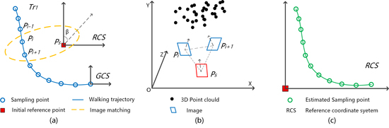
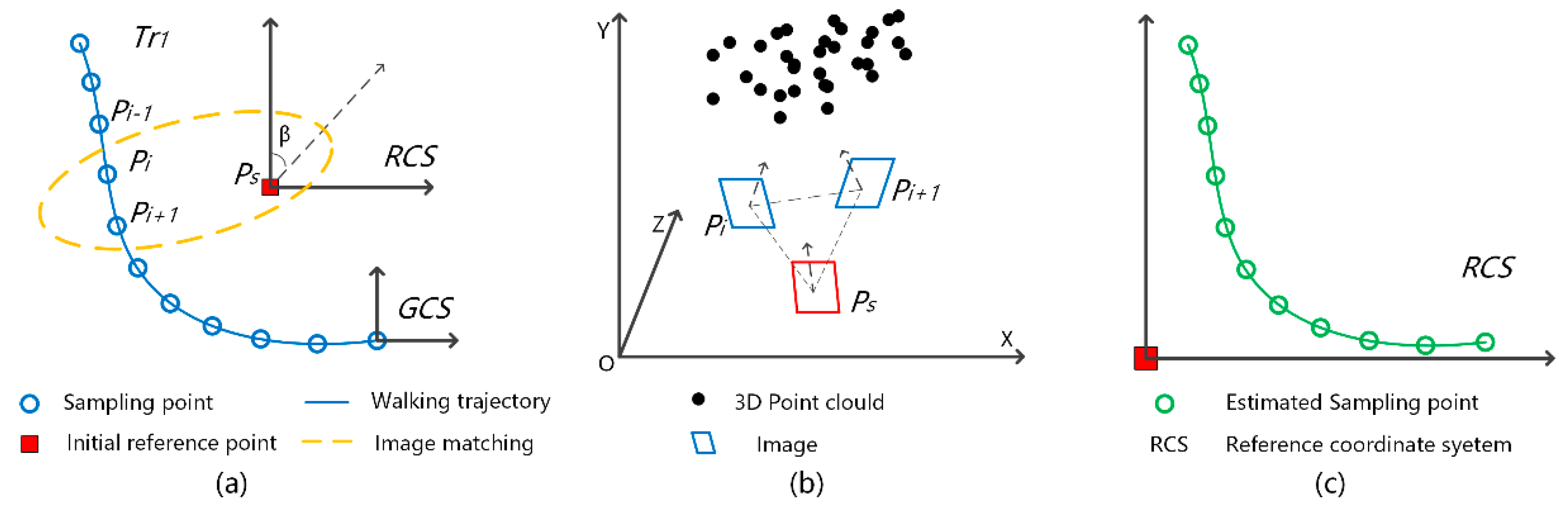
2. Visual Based Trajectory Geometry Recovery

Figure 1 illustrates the framework of this method. Smartphones are used to collect various sensor data, including video frames, inertial sensors data, Wi-Fi RSS, etc. In this study, some volunteers are required to collect the experiment data with smartphone. During data collection, the volunteers hold a smartphone in hand and walk normally in an indoor area. Firstly, a trajectory reconstruction method was designed to geometrically recover the trajectories from the corresponding crowdsourcing data. Heading angle estimation, step detection and step length estimation are the necessary steps for recovery of trajectory geometry. Both the video frames and the inertial data were employed in order to improve the accuracy of trajectory geometry recovery. Image matching and structure from motion (SFM) methods were used to calculate heading direction of trajectory geometry. This method can recover relative location of trajectory sampling points without prior knowledge, such as floorplan or initial location of the trajectory. After trajectory geometry recovering, a trajectory calibration algorithm was proposed to spatially estimate the location of trajectory in the RCS. By using the initial reference point (IRP), the trajectory geometry can be calibrated into RCS. Importantly, sampling points from the calibrated trajectory can be used as supplementary reference points for the following crowdsourced trajectories. Finally, the sensor data that are associated with the sampling points (from the calibrated trajectories) can be used for the mapping of different database, such as Wi-Fi radio map or image database with spatial labels.

During trajectory geometry recovery, the accurate estimation of heading angle of each sampling point from a trajectory is an important issue. The estimations by employing angular velocity (from gyroscope) are usually not accurate due to the drift error of smartphone sensors and the accuracy degradation over time [38]. The method that is proposed in this study uses an SFM-based method for the estimation of heading angle by using video frames. A sliding-window filter-based algorithm is proposed to improve further the performance of heading angle estimation. Finally, the geometry of a trajectory can be recovered by integrating the heading angle of each sampling point and the distance between every pair of adjacent sampling point.

The proposed approach aims to estimate, at every sampling instant t, the pose of sampling point $s_t=\left(x_t,y_t,{\theta }_t\right)$ with regard to the initial pose $s_0$, where $\left(x_t,y_t\right)$ represents the position of $s_t$ relative to the initial position $\left(x_0,y_0\right)$, and ${\theta }_t$ is the orientation of $s_t$ relative to the initial heading angle ${\theta }_0$. Note that the initial pose $s_0$ is unknown for each trajectory. Section 3 describes the spatial estimation of a trajectory in a coordinate system.

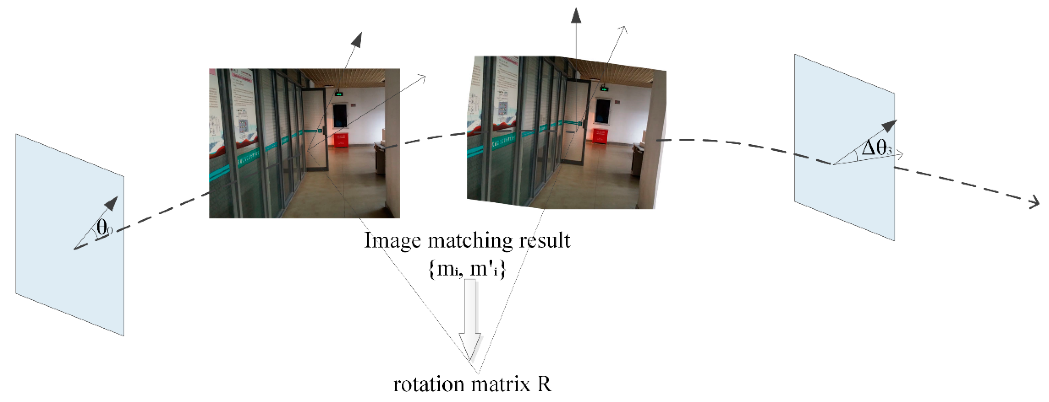
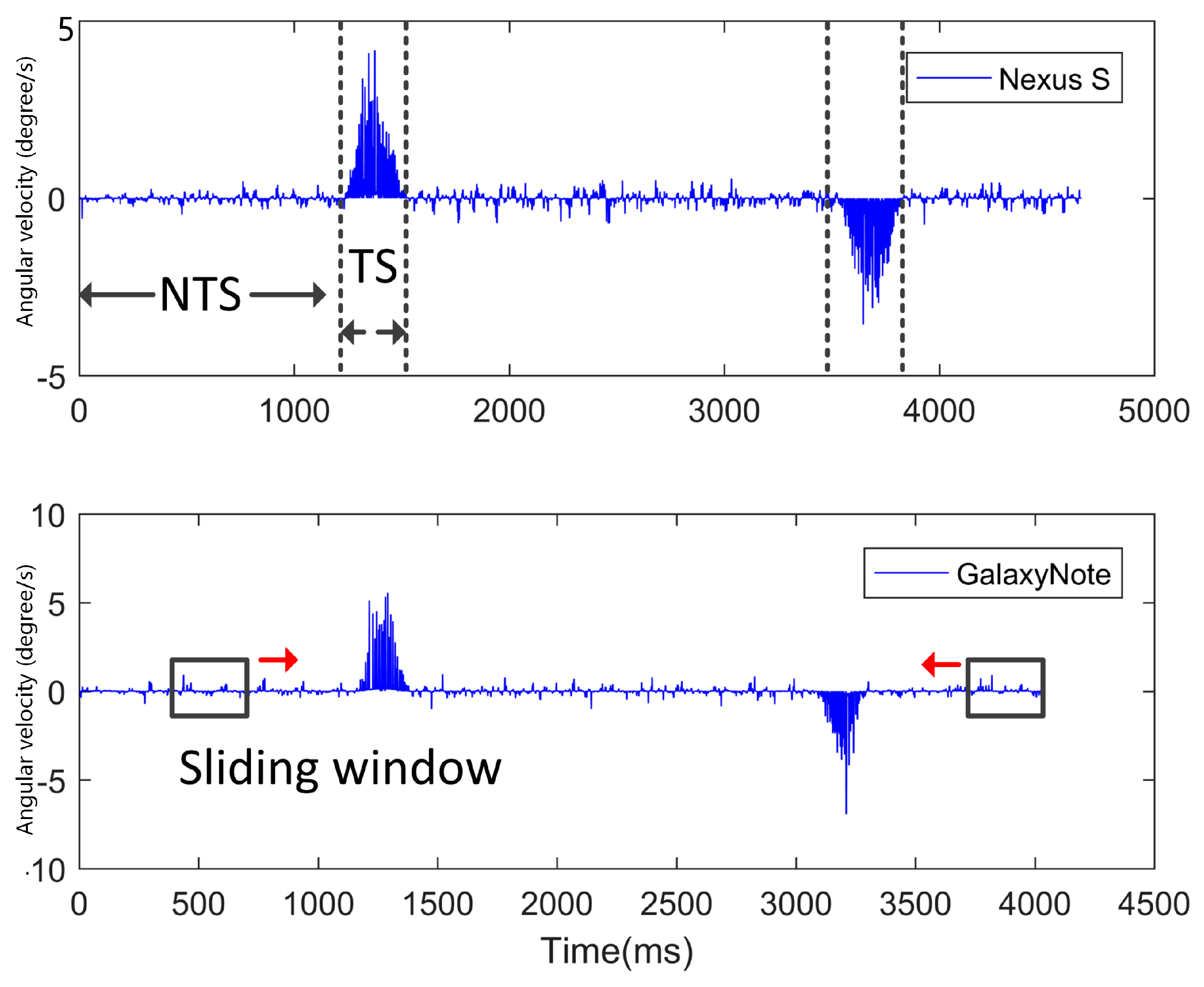
2.1. Heading Angle Estimation

The main idea of this method is that the heading angle of a sampling point can be represented by the heading angle of the image taken at this sampling point. Therefore, the heading angle change of a sampling point sequence can be estimated by calculating the heading angle change of the corresponding image sequence that is extracted from video frames. Similar to [8,11], we use the SFM-based method to estimate the heading angle change in sampling points from a trajectory. An image matching method was implemented on two adjacent images from image sequence. For a pair of images, the homogeneous matching points are used for calculating the fundamental matrix F:

$$\left[u_i^{\prime },v_i^{\prime },1\right]·F·\left[\begin{array}{c}{u}_i\\ v_i\\ 1\end{array}\right]=0$$

(1)

where $m_i{\left(u_i,v_i,1\right)}^T$, $m_i^{\prime }\left(u_i^{\prime },v_i^{\prime },1\right)$ are the homogeneous matching points from the image matching result $\left\{m_i,m_i^{\prime }|i=1,2,\dots n\right\}$, F is a $3\times 3$ order matrix. It is possible to linearly calculate the matrix F if there are enough matched points [39]. After obtaining the fundamental matrix, the essential matrix E can be calculated as:

$$\mathrm{E}=K^{T}FK$$

(2)

where K is the intrinsic matrix of a smartphone camera, which can be obtained based on the MATLAB Camera Calibrator (MATLAB 8.x on Windows) [40]. The rotation matrix R can be calculated by utilizing singular value decomposition (SVD) of essential matrix E. Importantly, the heading angle of a sampling point can be expressed by a rotation matrix:

$$R=\left[\begin{array}{ccc}cos\Delta \theta & 0& sin\Delta \theta \\ sin\Delta \vartheta sin\Delta \theta & cos\Delta \vartheta & -sin\Delta \vartheta cos\Delta \theta \\ -cos\Delta \vartheta sin\Delta \theta & sin\Delta \vartheta & cos\Delta \vartheta cos\Delta \theta \end{array}\right]$$

(3)

where $\Delta \theta$ is the heading angle change of sampling point $P_t$ relative to the last sampling point $P_{t-1}$. The schematic diagram of this SFM-based heading angle estimation method is shown in Figure 2. If the initial sampling point heading angle is ${\theta }_0$, the heading angle of sampling point $P_t$ can be calculated as:

$${\theta }_t={\theta }_0+{{\displaystyle \sum }}_{i=1}^{t-1}\Delta {\theta }_i$$

(4)

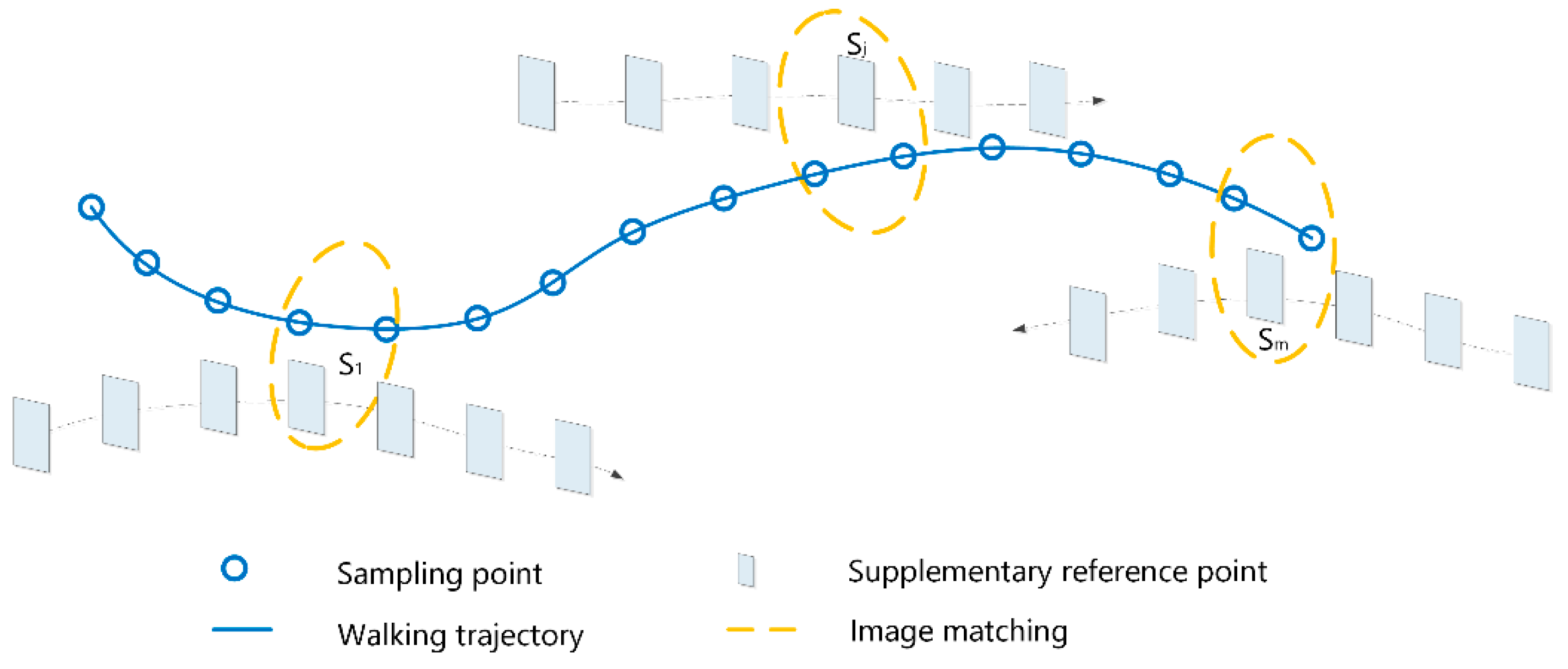
2.2. Trajectory geometry recovery

In this study, the aim of trajectory geometry recovery is to estimate the relative location of each sampling point from a trajectory. The relative location of a sampling point can be calculated, as follows:

$$\{\begin{array}{c}{x}_t=x_{t-1}+L·sin\left({\theta }_{t-1}+\Delta \theta \right)\\ y_t=y_{t-1}+L·cos\left({\theta }_{t-1}+\Delta \theta \right)\end{array}$$

(5)

where ($x_t, y_t$) is the location of sampling point $P_t$, ${\theta }_{t-1}$ is the heading angle of sampling point $P_{t-1}$, and $\Delta \theta$ is the heading angle change of $P_t$ that is relative to $P_{t-1}$. L is the distance between $P_t$ and $P_{t-1}$. The SFM-based heading angle estimation method can be used to calculate the $\Delta \theta$ of a sampling point, where accuracy of this method depends on the performance of image matching. The accuracy will be affected if the quality of video frames is poor. To solve this issue, the collected inertial data is also used to estimate the heading angle, which is independent from the visual estimation results.

Usually, smartphone gyroscope-based heading angle estimation can be calculated as integral of the angular velocity (rad/s) with respect to time. The frequency of smartphone gyroscope is more than 100 HZ, which is higher than video frame 30 fps. This method is only suitable for estimating heading angles in a short-term condition due to the drift error in smartphone gyroscope. With the increase in the integration time, the error of the heading angle rapidly and continuously grows. In order to avoid this problem, we have employed different strategies for different route segments. As shown in Figure 3, a pedestrian trajectory consists of two types of segments: turning segments (TSs) and non-turning segments (NTSs). A TS segment refers to a turning period with a relatively long turning time; an NTS segment refers to a straight (or approximately straight) walking period that may contain several slight turning actions with very short turning times. The strategy of our method is described as follows:

(1) for each TS sampling point (i.e., sampling points from a TS segment): the SFM-based method is used to estimate the heading angle if there is no image-matching failure.

(2) for TS sampling points with image-matching failure: the gyroscope-based method is used for heading angle estimation.

(3) for NTS sampling point: the lowest from two outputs (SFM-based and gyroscope-based) is used as the final output.

Based on the integration of the two sources, the robustness of the heading angle estimation method can be improved, especially when there is failure of image matching.

One important issue with this method is to accurately detect each turning moment (i.e., the joining point between each pair of TS segment and NTS segment) of a trajectory. When considering the high sampling rates (100 Hz) of gyroscope, this method uses gyroscope readings to detect turning moments. As shown in Figure 3, the angular velocity from an NTS segment fluctuates slightly around zero. However, for a TS segment, the angular velocity is always higher (or lower) than zero and the absolute value is much higher as compared to the NTS segment. According this regularity, a sliding-window filter is designed to detect the starting and ending moments of each turning action of a trajectory, detailed description can be found as follows:

Algorithm 1 Sliding-window filter-based turning moment detection

Input: gyroscope angles

Input: sliding window

Output: Turn[,]; //a two-dimensional vector which records the starting and ending moment of each TS segment of a trajectory

definition: size_win; //the size of the sliding window

count(); // The function to count the number of positive values or negative values

Pair(); // The function to find the starting and ending moment of each TS segment

Turn_S=[]; // The vector to record the candidate moments of start turning

Turn_E=[];// The vector to record the candidate moments of end turning

Np=0;// the number of angular velocity readings which are higher than 0

Ne=0;// the number of angular velocity readings which are below 0

for i=1:length(gyroscope angle)

sliding window=gyroscope angle[i,(size_win+i)];

Np=count(sliding window);

Ne=count(sliding window);

if Np==size_win || Ne=size_win

Turn_S.add(i);

end if

end for

for i=length(gyroscope angle):-1:1

sliding window=gyroscope angle[(i-size_win),i];

Np=count(sliding window);

Ne=count(sliding window);

if Np==size_win || Ne=size_win

Turn_E.add(i);

end if

end for

Turn=Pair(Turn_S, Turn_E);

The input of Algorithm 1 includes gyroscope-based heading angle estimations and a sliding window. The gyroscope-based angles are calculated by integrating the angular velocity readings with respect to the timespan between two sampling points. Similar to [41], the value of the sliding window was set to 50 in the experiment. The output of the Algorithm 1 is a two-dimensional vector Turn, which records the starting and ending moment for each TS segment. The main idea of Algorithm 1 is to monitor the fluctuation of gyroscope angles within the sliding window. If all of the gyroscope angles within the sliding window are in the same interval (>0^°or <0^°), the first moment of the sliding window can be treated as a candidate for the starting or ending moment of a TS segment, which are stored in vector Turn_S and Turn_E, respectively. For a TS segment, the first candidate in Turn_S is treated as its starting moment. Similarly, the first candidate in Turn_E is treated as its ending moment.

Based on the turning moment detection algorithm, the visual and inertial estimations can be integrated to calculate the heading angle for each sampling point from a trajectory. Walking steps can be detected by a peak and valley detection algorithm [38], which is an important step in restricting the distance between the adjacent sampling points. The length of each step can be estimated based on a Weinberg model [42]:

$$\mathrm{step}\_{\mathrm{length}}_i=K^4\sqrt{A_{max}-A_{min}}$$

(6)

where $\mathrm{step}\_{\mathrm{length}}_i$ is the length of the i-th step of a trajectory (i.e., ${\mathrm{step}}_i$), $A_{max}$ and $A_{min}$ are the maximum and minimum values of the Z-axis acceleration during one step period. K is the ratio of the real distance and the estimated distance. After the estimation of steps and step length, the location of the trajectory sampling points can be calculated. When considering the high sampling rate of gyroscope, we assumed the sampling points are equally spaced in a step. The distance between two sampling points from a trajectory can be calculated as:

$${\mathrm{distance}}_{t-1,t}=\frac{1}{n}step\_lengt{h}_i\hspace{1em}{P}_t,P_{t-1}\in S_i^P$$

(7)

where ${\mathrm{distance}}_{t-1,t}$ is the distance between two adjacent sampling points $P_t$ and $P_{t-1}$, which are in the i-th step of a trajectory. The $S_i^P$ is a set of sampling points within ${\mathrm{step}}_i$, n is the number of sampling points in $S_i^P$.

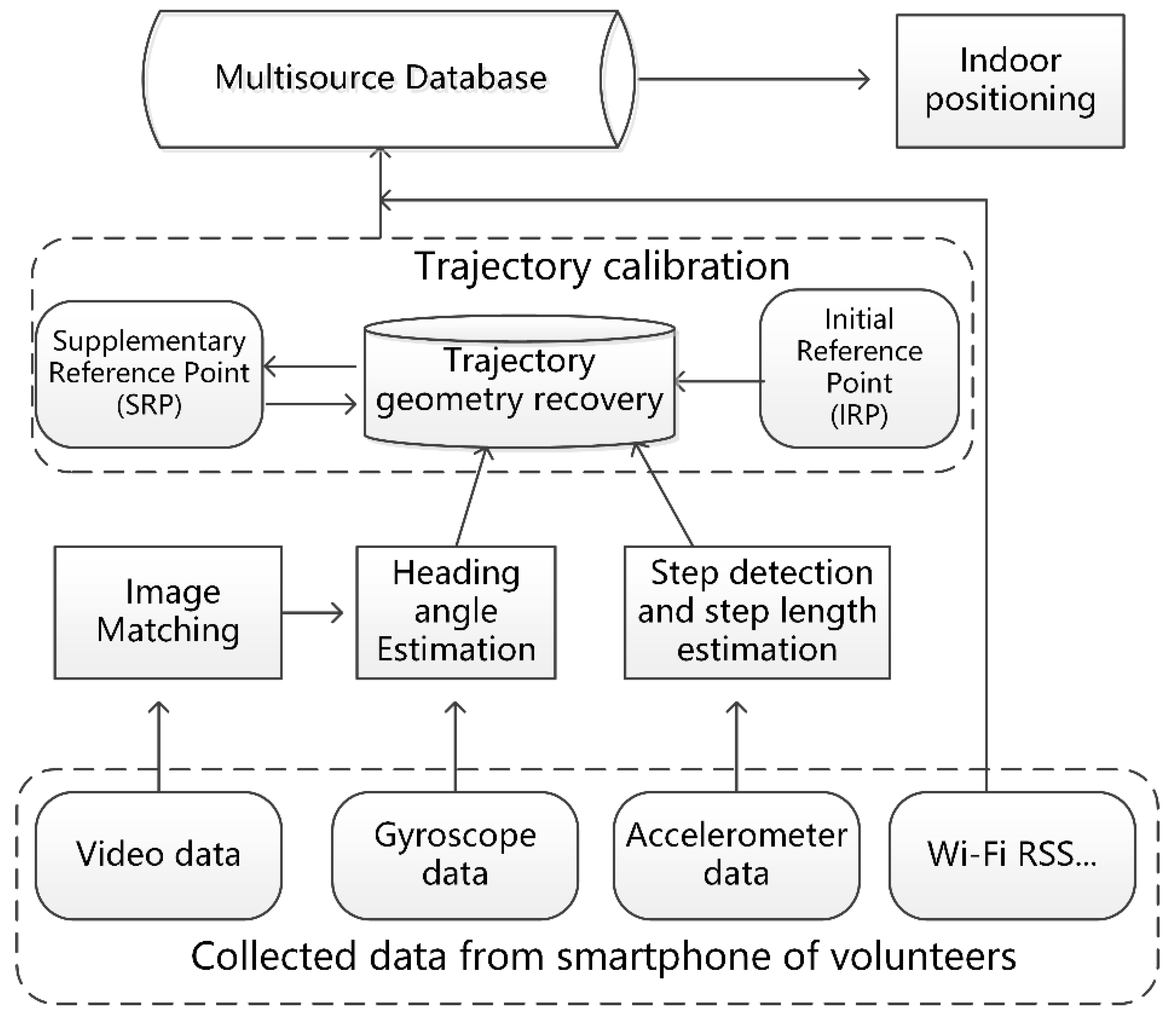
3. Trajectory Calibration and Geo-Tagging

In this section, a method is proposed to estimate spatial a trajectory in a reference coordinate system. Each sampling point from a trajectory can be geo-tagged while using an iterative algorithm. The geotagged sampling points, which are associated with the corresponding RSS and image data, can be used to construct multisource datasets for indoor localization.

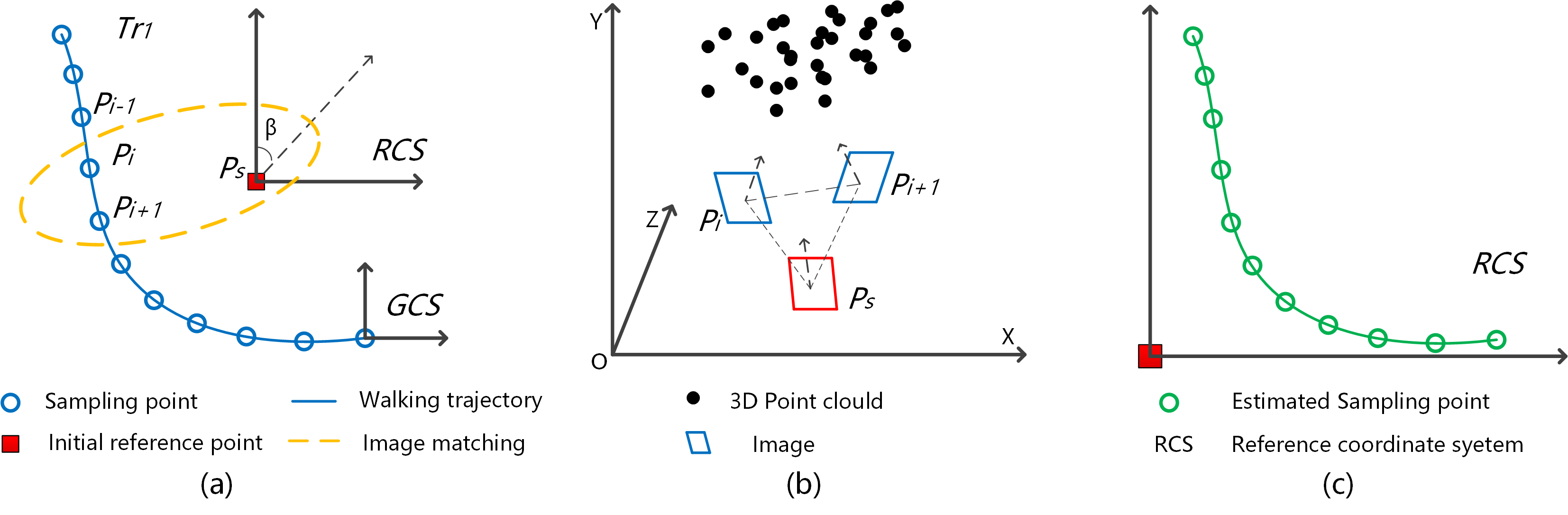
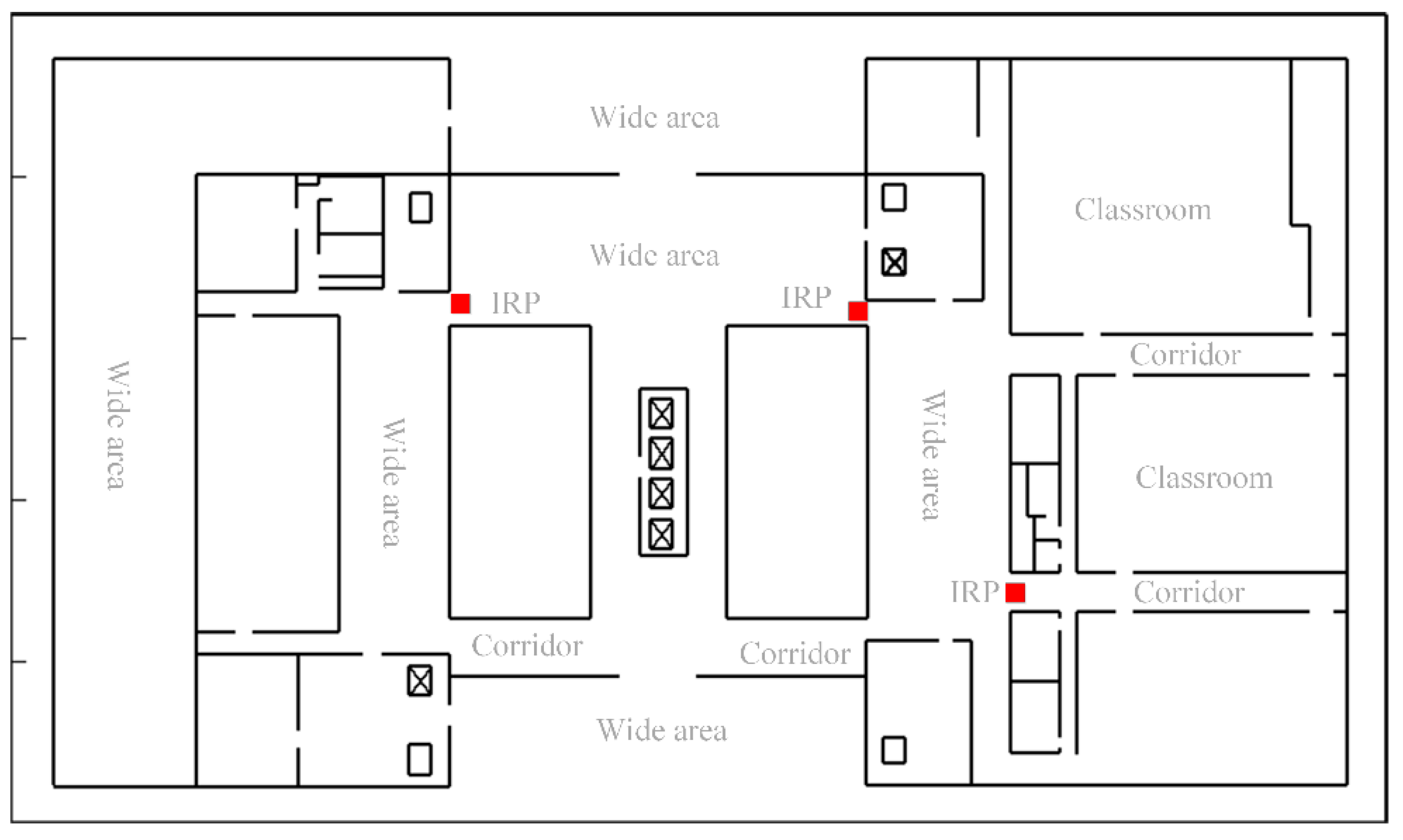
3.1. Indoor Reference Coordinate System

In most cases, indoor location-based services and applications mainly focus on the location of targets in the local coordinate system (e.g., inside a building), but not the location in a world coordinate system (e.g., WGS84). In this study, firstly, we define a trajectory geometry coordinate system (GCS), which represents the location of a trajectory relative to its initial location. It uses the initial location of a trajectory as its origin and the X and Y axes directly along the east and north, respectively. Subsequently, a two-dimensional reference coordinate system (RCS) is defined to determine the location of a point in the whole indoor space. It uses the location of an initial reference point (IRP) as its origin. Note that the IRP can be arbitrarily selected from an indoor space. For local applications (e.g., navigation services in a building), there is no need to measure its location in a world coordinate system. For global applications, the location of the whole indoor space can be estimated based on the global location of an IRP. The purpose of using IRP is to reduce the application difficulty for the geo-tagging method: it is difficult for many participants to measure the global location of the collected sampling points in a crowdsourcing condition. By using the IRP as an origin, the location of all the collected sampling points (from different participants) can be estimated in the RCS using the proposed algorithm. The location of an IRP needs to be measured once only. For the geo-tagging algorithm, several images are collected at the IRP (in different directions) and they are used as reference images. The algorithm can also be implemented in a multiple IRP condition. The influence of the number of IRP will be evaluated in Section 4. Prior knowledge, such as a floorplan or the initial location of the crowdsourced trajectories, is not required for the geo-tagging algorithm.

The main idea of this algorithm is to determine whether a trajectory crosses a reference point by matching image keypoints between the reference images (images of reference points) and the sampling images (images from a trajectory). If there is a matching success, the location of the sampling points (from the trajectory) can then be estimated in the RCS by using the bundle adjustment (BA) algorithm [43]. More importantly, the spatially estimated sampling points can also be used as reference points, called supplementary reference points (SRPs), to estimate the location of the sampling points from the following trajectories. The sampling images of the SRPs can be directly used as their reference images. The coverage of reference points, including IRPs and SRPs, continuously increases with the increase in crowdsourced trajectories, which makes the algorithm more efficient and robust.

3.2. Geo-Tagging Sampling Points in Reference Coordinate System

To geo-tag sampling points from a trajectory, keypoints from each sample image are matched against those from the reference images (i.e., reference images of IRPs and SRPs) by using the image matching technique that is detailed in Section 2. If the number of successfully matched keypoints is higher than a threshold r, the reference point is used to estimate the location of each sampling point (from the trajectory) by using a BA method. The main idea of BA is to calculate the three-dimensional (3D) location of keypoints and to refine the relative location between images by minimizing the projection error of the keypoints and the tracked keypoints on the images. The result of BA is the optimal 3D location of keypoints and the relative pose among the cameras. The spatial relation between a reference point and a sampling point can be represented by the cameras’ relative pose that is calculated by the use of BA. If a sampling point is successfully matched with reference point, the location of all the sampling points from the trajectory can be estimated in the RCS. The sampling points from the estimated trajectory will be used as SRPs for the following trajectories.

As shown in Figure 4a, Tr1 is a trajectory, and its geometry has been reconstructed by using the method that is proposed in Section 2. An image-matching method is used to find the best matching result (with the highest number of matched keypoints) between the sampling point image $P_i$ and the initial reference point image $P_s$. Note that its adjacent sampling point $P_{i+1}$ will also be selected as a candidate that may across the IRP $P_s$ if the matching result between $P_{i+1}$ and $P_s$ is higher as compared to $P_{i-1}$ and $P_s$. Otherwise, $P_{i-1}$ is selected. In Figure 4b, the optimal 3D point cloud and the relative location among $P_i$, $P_{i+1}$, and $P_s$ are calculated based on the BA method. After the BA process, the 3D coordinates of the two sampling points are: ($x_i$, $y_i$, $z_i$), ($x_{i+1}$, $y_{i+1}$, $z_{i+1}$), respectively. The 3D coordinates should be transformed to the coordinates in the RCS due to the lacking of scale information for the BA method. The scale parameter between the two coordinate systems can be calculated, as follows:

$$\mathsf{\sigma }=\frac{\mathrm{D}\left(\mathrm{i},\mathrm{i}+1\right)}{\sqrt{{\left(x_i-x_{i+1}\right)}^2+{\left(y_i-y_{i+1}\right)}^2+{\left(z_i-z_{i+1}\right)}^2}}$$

(8)

where $\mathsf{\sigma }$ is the scale parameter of BA, $\mathrm{D}\left(\mathrm{i},\mathrm{i}+1\right)$ is the distance between $P_i$ and $P_{i+1}$. Therefore, the coordinates of a sampling point $P_i$ in the RCS can be calculated, as follows:

$$\left[\begin{array}{c}{X}_i\\ Y_i\end{array}\right]=\mathsf{\sigma }\left[\begin{array}{cc}cos\beta & sin\beta \\ -sin\beta & cos\beta \end{array}\right]\left[\begin{array}{c}{x}_i^{\prime }\\ y_i^{\prime }\end{array}\right]$$

(9)

where ($X_i,Y_i$) is the coordinates of $P_i$ in the RCS, $\beta$ is the heading angle of the matched reference image of IRP $P_s$, and ($x_i^{\prime },y_i^{\prime }$) is the two-dimensional (2D) projection of the 3D coordinates ($x_i$, $y_i$, $z_i$) in the RCS. In equation (9), the coordinates of $P_{i+1}$ in the RCS are represented as ($X_{i+1},Y_{i+1}$). The coordinate of $P_i$ and $P_{i+1}$ in Section 2 can be calculated as ($g{x}_i,g{y}_i$) and ($g{x}_{i+1},g{y}_{i+1}$). The transformation parameters, including the rotation angle $\vartheta$ and the shiftings (${\mathrm{t}}_x$, ${\mathrm{t}}_y$), can be calculated according to the coordinates of $P_i$ and $P_{i+1}$ in the GCS and the RCS [44]. Based on the location estimation results of $P_i$, the location of each sampling point from the trajectory can be estimated in the RCS, as follows:

$$\left[\begin{array}{c}{X}_i\\ Y_i\end{array}\right]=\left[\begin{array}{c}{\mathrm{t}}_x\\ {\mathrm{t}}_y\end{array}\right]+\left[\begin{array}{cc}cos\vartheta & sin\vartheta \\ -sin\vartheta & cos\vartheta \end{array}\right]\left[\begin{array}{c}g{x}_i\\ g{y}_i\end{array}\right]$$

(10)

where ($X_i,Y_i$) is the coordinates of the sampling point in the RCS, ($g{x}_i,g{y}_i$) is the coordinates of the sampling point in the GCS. Figure 4c shows an example of a recovered trajectory in the RCS.

Once a trajectory has been estimated successfully in the RCS, its sampling points can be used as SRPs. This type of reference points is used to estimate the trajectories that do not cross IRP. As shown in Figure 5, a trajectory may cross multiple SRPs from different trajectories. To increase the robustness of this method, the location of a trajectory is calculated as the average of the estimation results by using each SRP. For example, utilizing supplementary reference point $S_1$, the coordinates of the sampling points can be calculated as {($X_1^1$, $Y_1^1$), ($X_2^1$, $Y_2^1$)…($X_k^1$, $Y_k^1$)}, where k is the number of sampling points in this trajectory. For example, using SRP $S_j$, the coordinates of each sampling point from a trajectory can calculated as: {($X_1^j$, $Y_1^j$), ($X_2^j$, $Y_2^j$)…($X_k^j$, $Y_k^j$)}, where k is the number of sampling points from this trajectory. If there are m SRPs, the coordinates of a sampling point can be estimated in the RCS, as follows:

$$\{\begin{array}{c}{X}_i=\frac{1}{m}\left(X_i^1+X_i^2+\cdots +X_i^m\right)\\ Y_i=\frac{1}{m}\left(Y_i^1+Y_i^2+\cdots +Y_i^m\right)\end{array} i\in \left[1,k\right]$$

(11)

where ($X_i,Y_i$) is the coordinates of the i-th sampling point, m is the number of SRPs that cross the trajectory.

The algorithm for trajectory estimation in the RCS is described in Algorithm 2. The inputs of this algorithm include N trajectories (geometry recovered), and at least one IRP where estimated trajectories are the outputs in RCS. The number of available SRPs continuously increases as the iteration of the algorithm. The algorithm ends when all trajectories are estimated.

Algorithm 2 Trajectory estimation in the RCS

input: N trajectories with recovered geometry

input: IRP[] //initial reference point

output: Estimated trajectories in the RCS

definition: Multi-IM() is the multi-constrained image-matching function, which returns the number of matched keypoints.

BA() is a bundle adjustment function which returns the location of two adjacent sampling points relative to an IRP

SRP=[]; // supplementary reference point

Label_trajectory=[]; //label a trajectory if it has been estimated in the RCS

While true

for ss=1:length(IRP)

for i=1 to N

if i does not exist in Label_trajectory

NUM=the number of sampling points of trajectory{i}

candidate=[];

for k=1 to NUM

n=Multi-IM(point{k}, IRP{ss}); // returns the number of matched keypoints

if n>r //the number of matched keypoints is higher than threshold r

candidate.add(point{k});

end if

if SRP.size>0

n=Multi-IM(point{k}, SRP);

if n>r //the number of matched keypoints is higher than threshold r

candidate.add(point{k});

end if

end

end for

flag=0; //label whether the two sampling points have been estimated in the RCS

for j=1: candidate

if points k and (k+1) exist in candidate[]

dist= || point{k}, point{k+1} ||; //calculate the distance between point{k} and point{k+1}

BA(point{k}, point{k+1}, dist, IRP); //calculate the relative location of point{k} and point{k+1} by using the bundle adjustment function

flag=1;

end if

if flag==1

estimate the trajectory{i} in the RCS;

SRP.add (sampling points of trajectory{i});

Label_trajectory.add(i);

break;

end if

end for

candidate.clear();

end if

end for

end for

if Label_trajectory.number==N

break;

end

end while

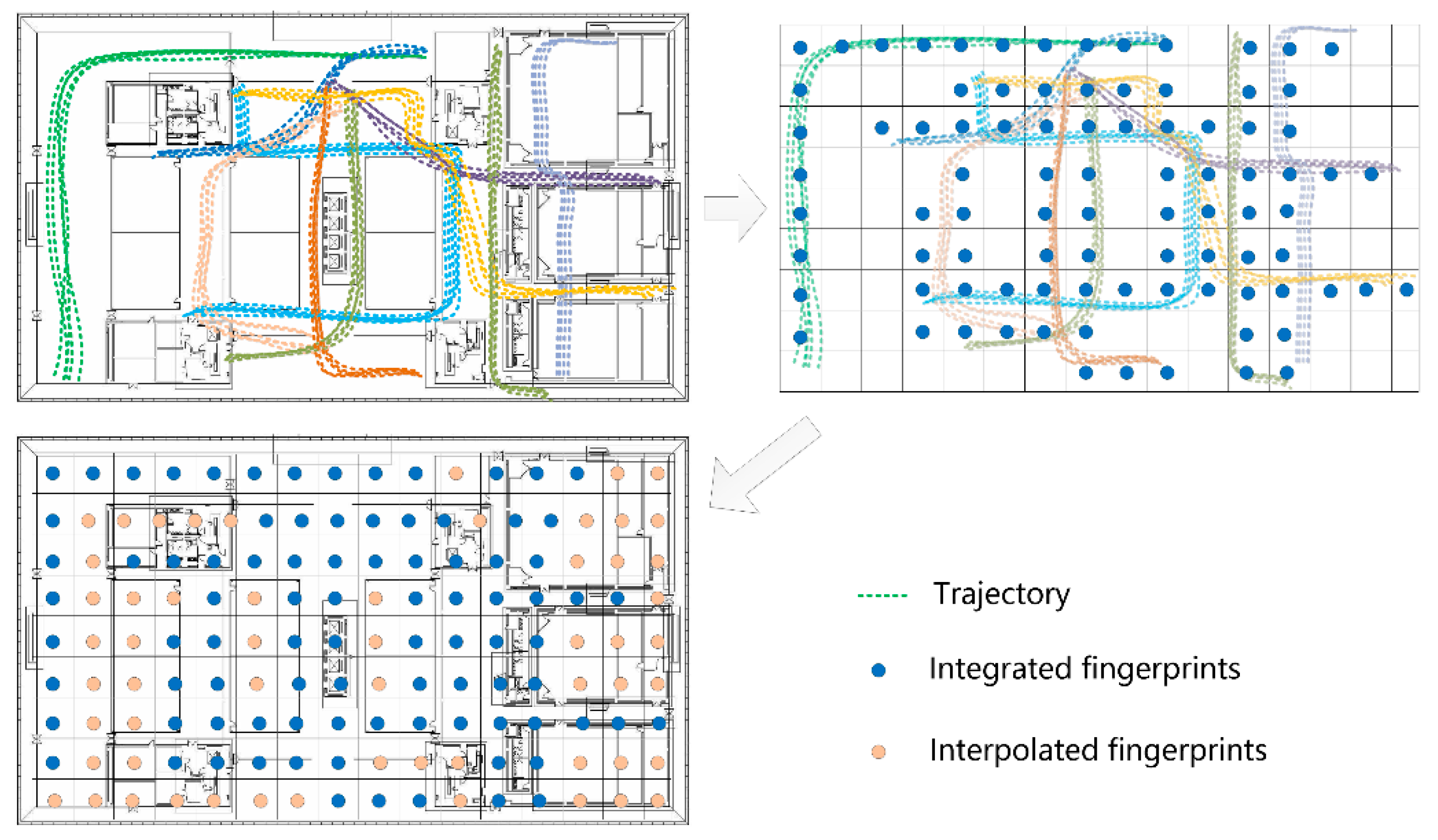
3.3. Generating Multi-Source Datasets for Indoor Positioning

After geo-tagging, the sampling points from crowdsourced trajectories can be used to generate datasets, including Wi-Fi radio map and geo-tagged image datasets.

Table 1. The attributes of the sampling points.

Sampling Point ID	Trajectory ID	Coordinates	RSS	Image	Direction
P1	Tr_1	$\left(X_1,Y_1\right)$	{($rs{s}_1,a{p}_1$), ($rs{s}_2,a{p}_2$)…}	I1	Azimuth1
P2	Tr_2	$\left(X_2,Y_2\right)$	{($rs{s}_1,a{p}_1$), ($rs{s}_2,a{p}_2$)…}	I2	Azimuth2
P3	Tr_3	$\left(X_3,Y_3\right)$	{($rs{s}_1,a{p}_1$), ($rs{s}_2,a{p}_2$)…}	I3	Azimuth2

shows the attributes of sampling points. The collected images, which are associated with their spatial location and direction attributes, can be directly used to generate geo-tagged image datasets. In order to reduce the time cost required for image matching-based indoor localization, a spatial index is constructed for the geo-tagged images.

In order to construct Wi-Fi radio map, an indoor space can be partitioned into many regular grids. The center of a grid is treated as the location of a Wi-Fi fingerprint. As this method is designed for crowdsourcing-based data collection and localization systems, it is assumed that the spatial distribution of fingerprints in an indoor space is not equal. Some grids may be passed through by multiple crowdsourced trajectories. Additionally, some grids may not be covered by any trajectory. In the first condition, the sampling points from all related trajectories can be integrated to generate fingerprints, we defined as integrated fingerprint. If there are m sampling points within the spatial extent of a grid, the RSS of AP i for this grid can be calculated, as follows:

$${\mathrm{rss}}_i=\frac{1}{m}{{\displaystyle \sum }}_{k\in G}rs{s}_i^k$$

(12)

where ${\mathrm{rss}}_i$ is the RSS value of AP i, G is the set of AP in the grid, $rs{s}_i^k$ is the ${\mathrm{rss}}_i$ of the k-th sampling point. If a grid does not contain any sampling point, we defined as interpolated fingerprint, the RSS of this grid can be interpolated by using its four-neighborhoods:

$${\mathrm{rss}}_i=\frac{{{\displaystyle \sum }}_{j}w\left(d_j\right)·RSS\left\{\right\}}{{{\displaystyle \sum }}_{j}w\left(d_j\right)}$$

(13)

where ${\mathrm{rss}}_i$ is the interpolated RSS value of AP i, $RSS\left\{\right\}$ is the four-neighborhoods grid of interpolated fingerprint, j is the index of a grid, d is the distance between interpolated fingerprint and grid j, $w\left(x\right)$ is the weight function which inverse the distance. The purpose of interpolation is to generate a radio map for indoor localization when space has not been completely covered by crowdsourced sampling points. The interpolated RSS of a grid will be replaced by an actual measured RSS when it is covered by the following trajectories.

4. Evaluation

In this section, several experiments are designed to evaluate the performance of the proposed method for indoor geo-tagging and positioning. As shown in Figure 6, a typical indoor environment with 106$\times 61$ m was selected as the experimental area with long corridors and wide areas. Two android based smartphones (SUMSUNG and HUAWEI) were used for collecting data, including inertial data, video frames and Wi-Fi RSS. The sampling rates of inertial data was 100 HZ, and the sampling frequency of video frame was 30 frames per second (FPS). During data collection, five volunteers (three males and two females) were invited to collect the experimental data. There are 10 different trajectories and each volunteer performed two trajectories. The participants held a smartphone vertically in front of them and kept the camera forward facing. Three IRPs were selected from the experimental area, as shown in Figure 6.

After data collection, the geometry recovery and geo-tagging of the trajectories were performed offline while using a laptop (4-core i7 CPU and 8G RAM). Based on the result of trajectory calibration and geo-tagging, a Wi-Fi radio map and a geo-tagged image dataset were constructed. An RSS based localization and an image based localization experiments were performed to evaluate the quality of the geo-tagged datasets.

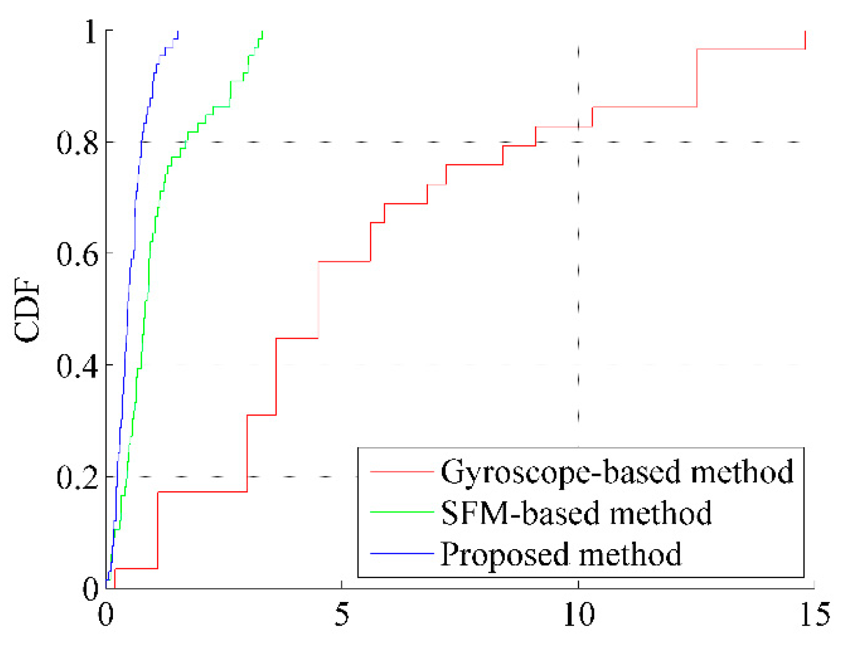
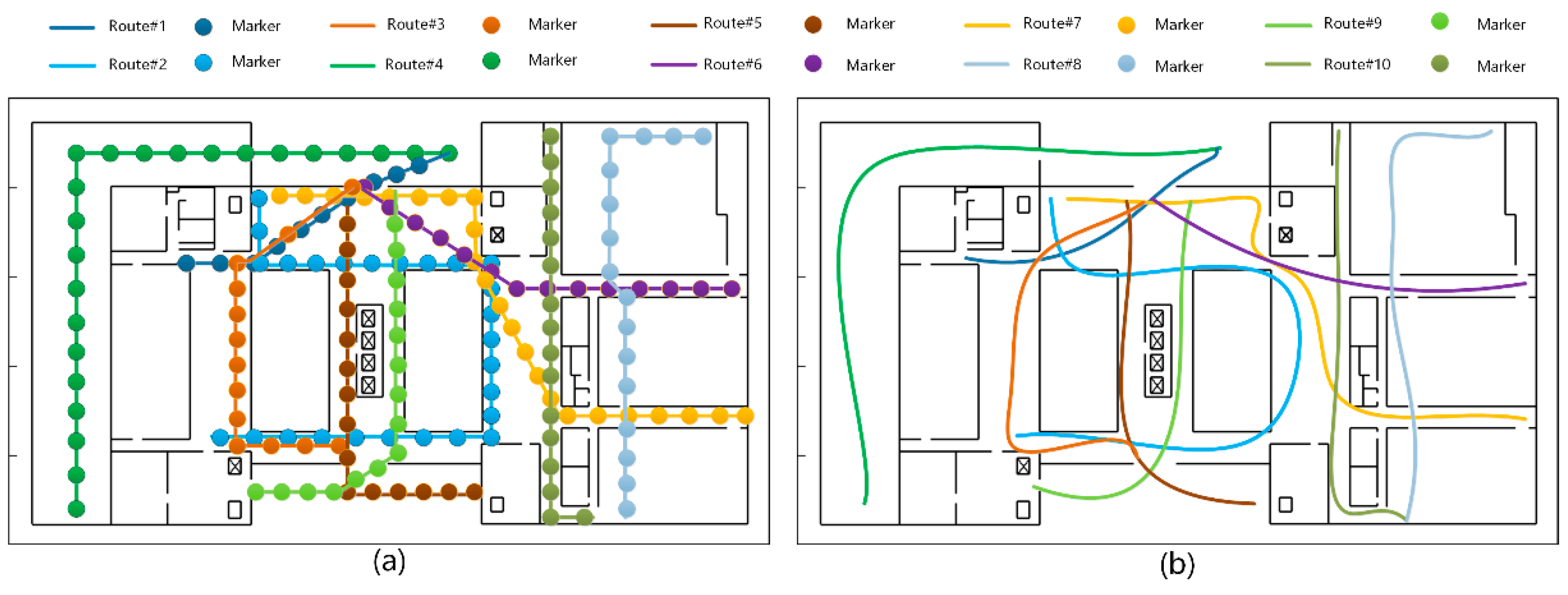
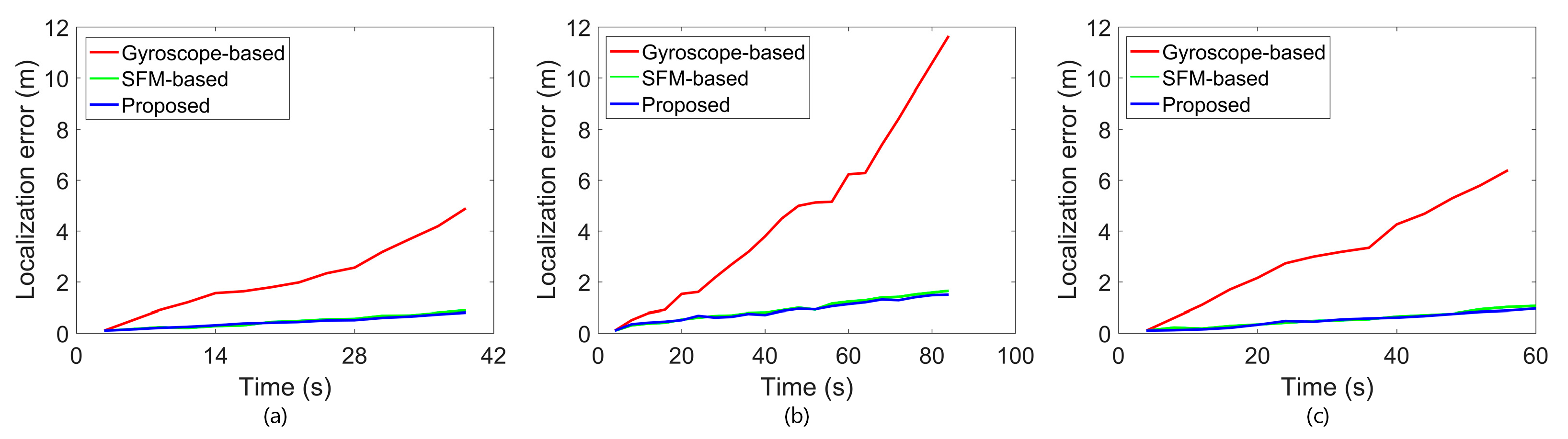
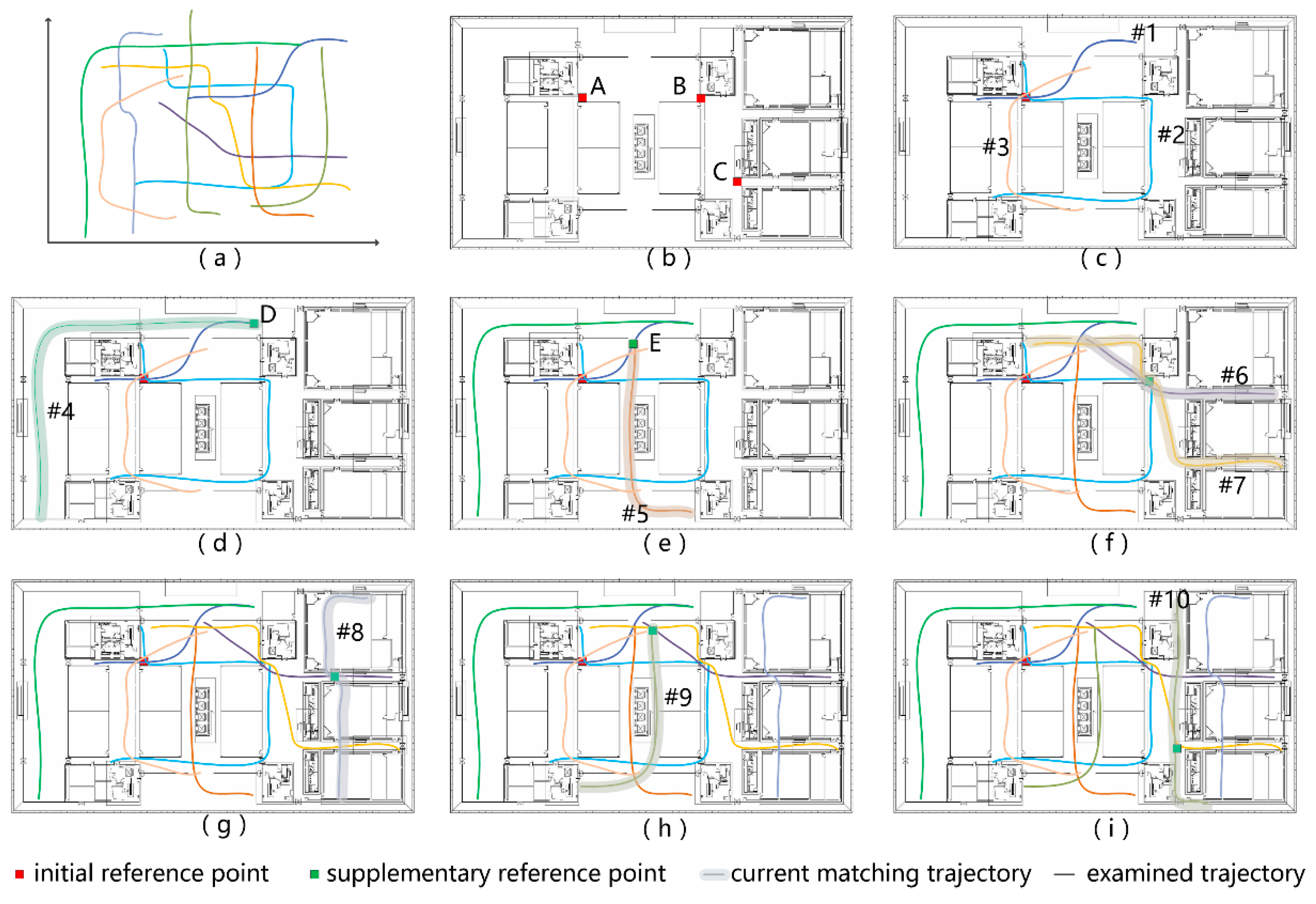
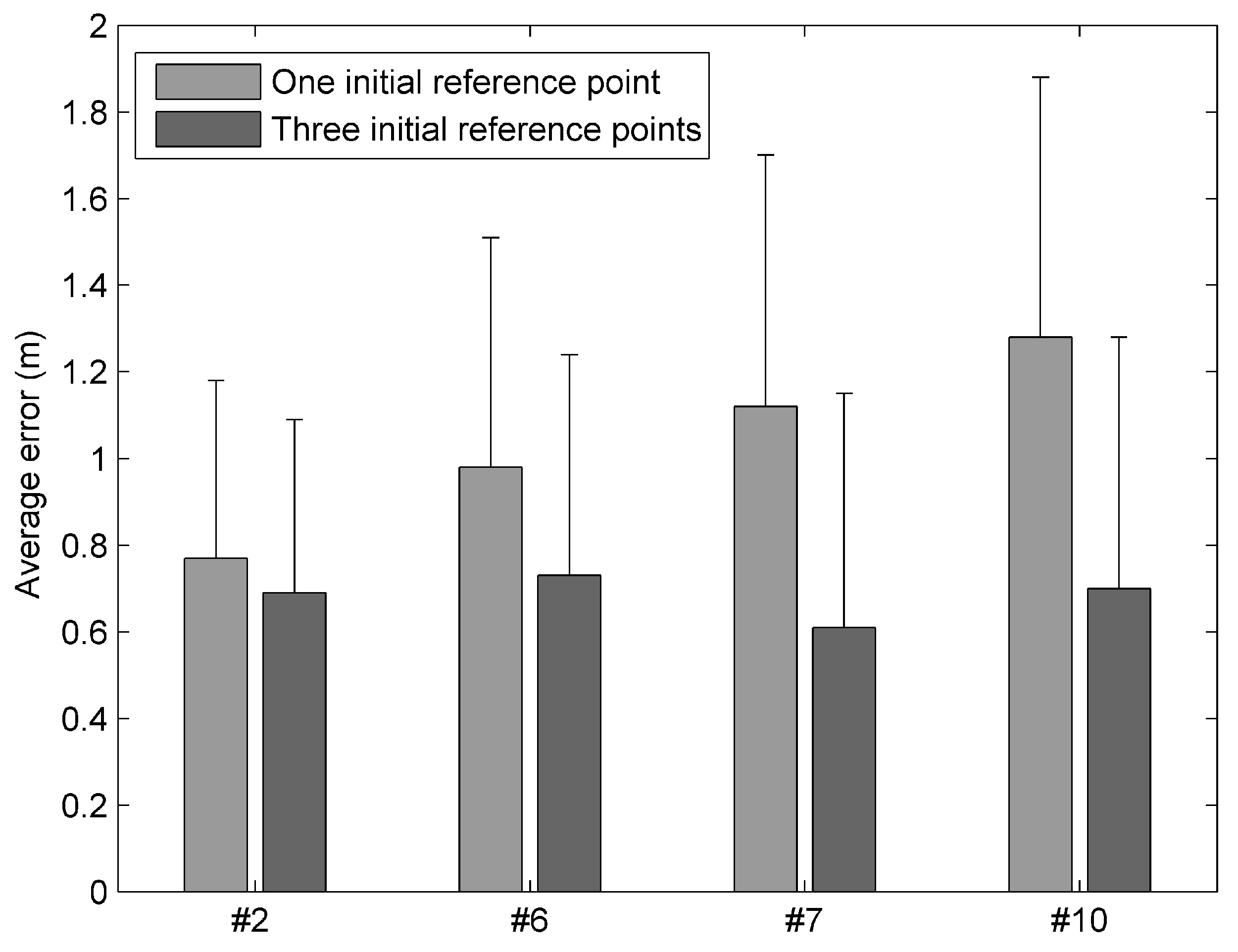
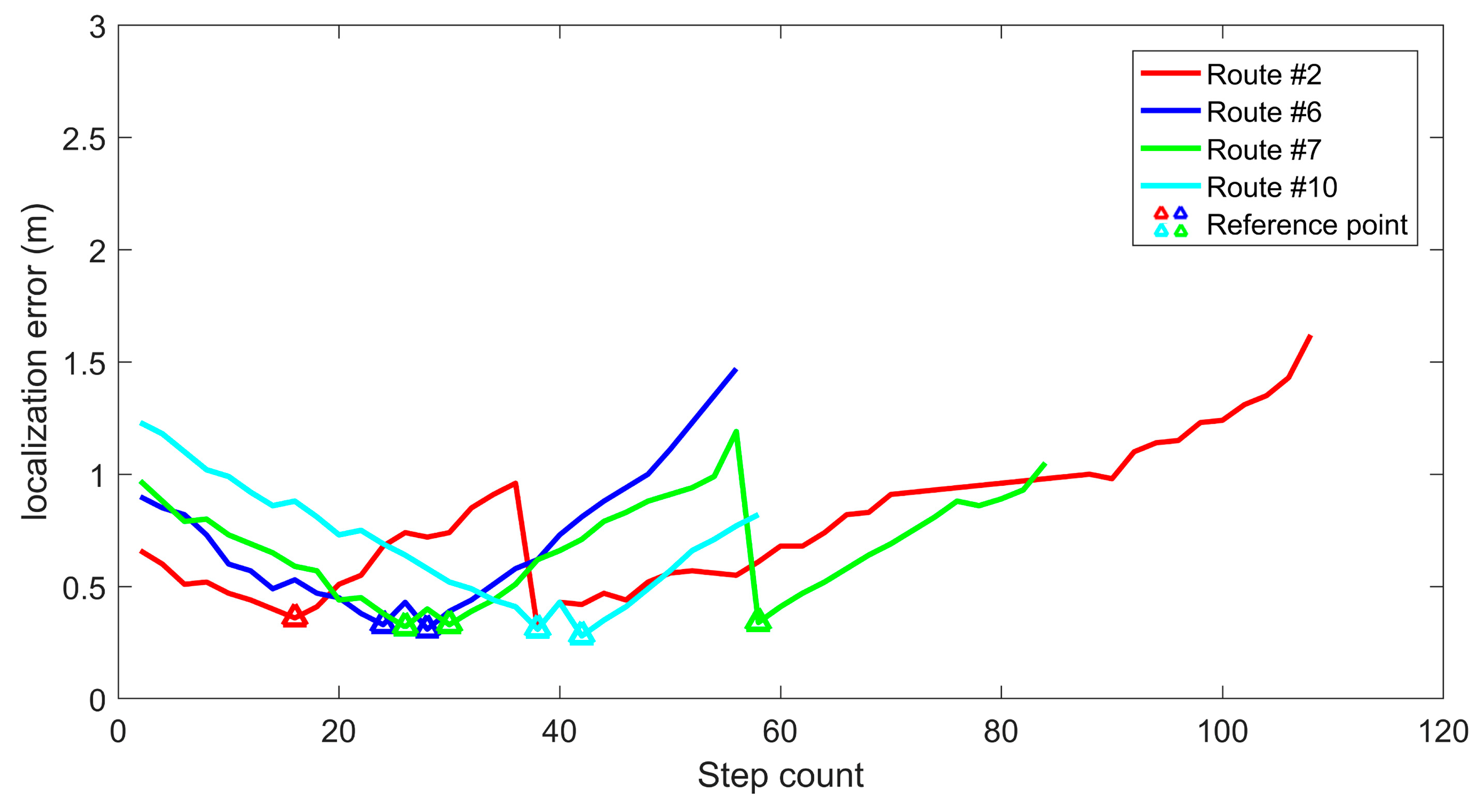
4.1. Evaluation of Trajectory Estimation

In this experiment, ten different trajectories were collected in the study area. As shown in Figure 7a, some markers with known location were set along each trajectory to collect the ground-truth data. The visual results of trajectories recovering are shown in Figure 7b. The average geo-tagging error of sampling points from ten trajectories is around 0.6m, the standard deviation of location error is about 0.4 m. The computation time of recovering 10 trajectories geometry is about 5.7 min.

The results were compared with gyroscope-based method and the SFM-based method in order to further evaluate the performance of the geometry recovery method. The gyroscope based method only uses the gyroscope data from smartphone to calculate the heading angle and restore walking trajectory. The SFM-based method employs a SFM process to estimate the heading angle using video frames. The shape discrepancy metric (SDM) [45] was used to verify the accuracy of these methods, which is defined as the Euclidean distance between a sampling point and its corresponding ground-truth point. Figure 8 shows the cumulative distribution function (CDF) of the SDM for 10 trajectories while using the three methods. The SDM error in gyroscope-based method is much higher as compared to other methods. For the SFM-based method, the maximum SDM error is about 3 m; the 80-percentile SDM error is around 2 m; and, the mean SDM error is about 1.1 m. This indicates that visual information can help to improve the estimation performance of the trajectory recovery. Moreover, the SDM error can be further reduced by integrating both visual and inertial information: the maximum SDM error is about 1.5 m; the 80-percentile SDM error is around 1 m; and, the mean SDM error is about 0.6 m. Figure 9 shows the increasing speed of trajectory recovery error using different methods. Three routes (#1, #2, and #3) are taken as examples. As can be seen from the figure, the increasing speed of the SFM-based method and the proposed method is obviously slower than the gyroscope-based method. These results demonstrate that the fusion of the visual and inertial information helps to overcome the shortcomings in a single-source based method, e.g., drift error from the gyroscope or matching failure of images. Furthermore, the experimental trajectories covered wide spaces in the study area. The results demonstrate that this approach can perform well in a wide indoor space, which may be difficult for the PDR-based methods.

Using the algorithm proposed in Section 3, the recovered crowdsourcing trajectories can be geo-tagged in the RCS. Note that the initial locations of these trajectories were unknown for the algorithm. As shown in Figure 10b, three IRPs (points A, B, and C) were set in the study area. Each IRP was associated with 12 reference images (intervals of 30°). Firstly, the algorithm uses one IRP (A) to estimate these trajectories and evaluate the performance of geo-tagging. After that, the two others IRPs are also used to test the influence of the number of IRPs on trajectory estimation and geo-tagging.

The spatial estimation results of all trajectories are shown in

Table 2. The estimation results of 10 trajectories based on one IRP.

	IRP Trajectory			SRP Trajectory
Trajectory	#1	#2	#3	#4	#5	#6	#7	#8	#9	#10
max error (m)	1.35	1.42	1.28	1.45	2.1	2.39	2.52	2.85	3.05	2.98
min error (m)	0.2	0.36	0.3	0.32	0.67	0.77	0.68	0.65	0.72	0.58
avg error (m)	0.61	0.77	0.65	0.85	1.09	0.98	1.12	1.55	1.46	1.28
Length (m)	41.7	102.8	56.9	101.1	59.0	55.2	85.6	65.4	57.8	57.6
Time (s)	21	52	29	153	180	980	1505	924	435	1260

. The results were evaluated by the maximum, minimum, average estimation error of the ground-truth points, and the computation time of each trajectory. The average error of all the trajectories is 1.03 m. The computation time for estimating these trajectories is 9.3 min.

As shown in Figure 10, the trajectories that cross an IRP (e.g., trajectories #1, #2, and #3) are termed IRP trajectories. Similarly, the trajectories that cross SRPs are termed SRP trajectories (e.g., trajectories #4–#10). The maximum, minimum, and average error of the IRP trajectories (1.45 m for #3, 0.36 m for #2, 0.85 m for #3) are clearly smaller than those of the SRP trajectories (3.05 m for #8, 0.77 m for #5, 1.55 m for #7), respectively. Nevertheless, the average error of all the SRP trajectories is below 1.56 m, which suggested that the proposed algorithm could achieve reasonable estimation results under the condition of only one reference point. By using SRPs, the spatial location of the SRP trajectories can also be estimated in the RCS.

Figure 10c–i shows the estimation process of all the trajectories. IRP A was firstly used for the estimation of trajectories. As shown in Figure 10c, only three trajectories (#1, #2, and #3) crossed IRP A. By using the method described in Section 3.2, these trajectories were first estimated in the RCS and the sampling points from the trajectories can be used as SRPs. By verifying relation between examined trajectories (nos. #1, #2, #3) and unexamined trajectories (nos. #4–#10), it was found that trajectories #4 and #5 are intersected with trajectory #1 at SRPs D and E, respectively (Figure 10d–e). The sampling points from the newly examined trajectories can also be used as SRPs, which continuously increases the coverage of the reference points in the study area. Note that although trajectories #6 and #7 also intersected with trajectory #1, the intersection relationship were not detected by the algorithm. This may be due to the orientation of the sample images of trajectory #6 (or #7), as it was not consistent with trajectory #1. As shown in Figure 10f–i, after several iterations, the remaining trajectories were all calibrated in the RCS.

To test the influence of the number of IRPs on the trajectory estimation, two other IRPs (B and C) have been added to the environment, as shown in Figure 10b. Same trajectories were estimated by the algorithm by using three IRPs. The average error of all trajectories reduced from 1.03 m (one IRP) to 0.67 m (three IRPs). As shown in Figure 11, after addition of two IRPs, the average error of trajectories #2, #6, #7, and #10 reduced from 0.77 m, 0.98 m, 1.12 m, and 1.28 m to 0.69 m, 0.73 m, 0.61 m, and 0.7 m, respectively. Figure 12 shows the increasing speed of trajectory estimation error. Four routes (#2, #6, #7, and #10) are taken as examples. As can be seen from the figure, once a trajectory passes through a reference point, the location error obviously reduces. The results show that the increase in number of IRPs helps to further improve the performance of the trajectory estimation. However, more IRPs also require more workload for the collection of reference points, including their location and reference images. Accordingly, this may increase the difficulty of crowdsourcing-based indoor positioning systems. Therefore, it is practical to set IRPs at the places where most people walk past, such as indoor intersections and entrances/exits, to reduce the number of required IRPs for large indoor environments.

4.2. Performance of Constructed Databases for Indoor Positioning

The sampling points from calibrated trajectory can be used to construct multisource databases for indoor positioning. In this section, two experiments are conducted to evaluate the quality of the constructed datasets, including RSS-based positioning test and image matching based positioning test.

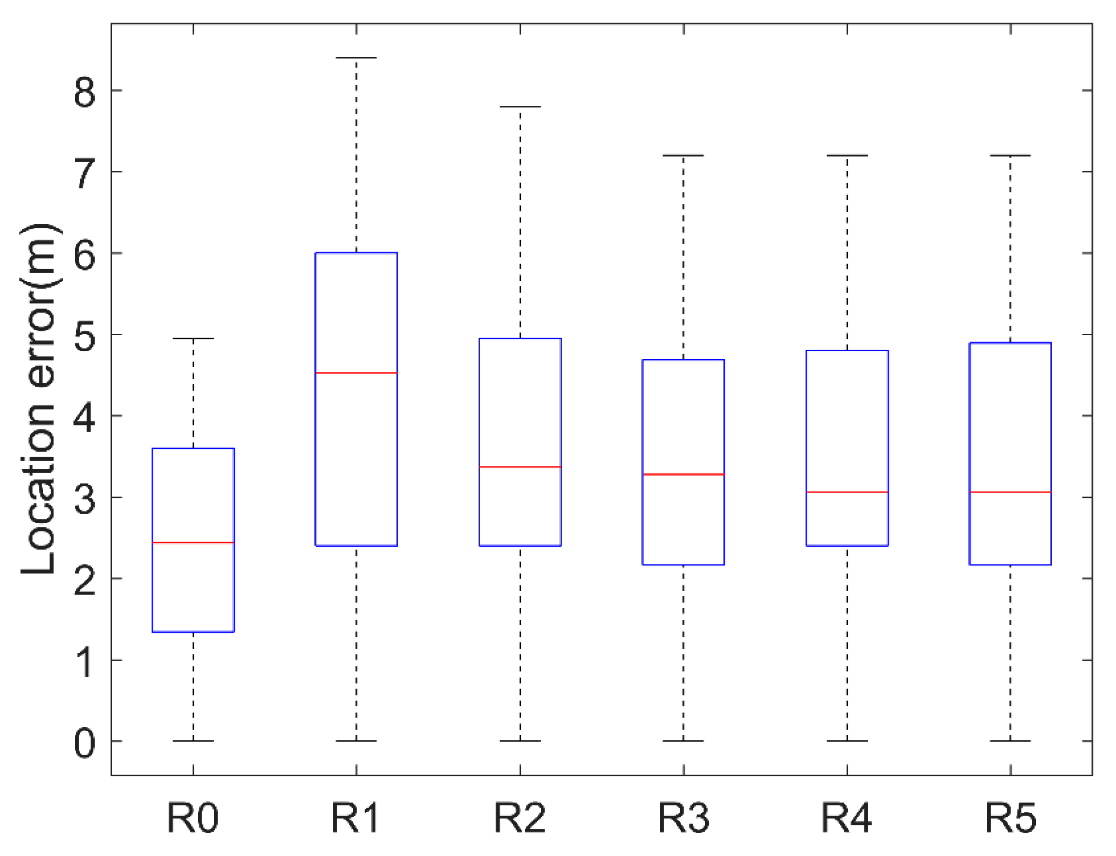
4.2.1. RSS-Based Indoor Positioning

Fifty calibrated trajectories (ten trajectories are shown in Figure 10, where each trajectory is repeated five times) were used to construct an indoor RSS database. The study area was partitioned into a 2.4 m × 2.4 m mesh grid. By using the method described in Section 3.3, the fingerprints were generated based on the integration of sampling points. The results of the fingerprint generation are shown in Figure 13. There were 89 integrated fingerprints (based on the integration of sampling points) and 55 interpolated fingerprints. Figure 14 shows the RSS distribution of two APs.

To evaluate the quality of the constructed RSS database, a positioning test was conducted based on a weighted k-nearest neighbor method at the 66 test points (the centers of 66 grids). Each grid was covered by more than five trajectories. The reason to select these grids was to verify the improvement in the quality of constructed radio map with increase in crowdsourced trajectories. For comparison, a site survey process was also conducted based on the same mesh grids. The positioning error was calculated, as follows:

$${\mathrm{Err}}_i=\sqrt{{\left(x_i^r-x_i^e\right)}^2+{\left(y_i^r-y_i^e\right)}^2}$$

(14)

where ${\mathrm{Err}}_i$ is the location error of point i, $\left(x_i^r,y_i^r\right)$ is the actual physical location of point i, and $\left(x_i^e,y_i^e\right)$ is the estimated physical location of point i.

Figure 15 shows the performance of the two methods (the site survey based method and the proposed method). R0 represents the localization error of the site survey based method. R1 to R5 represent the localization error of the proposed method. Here, R1 refers to the constructed radio map by using sampling points from one trajectory. Similarly, R2, R3, R4, and R5 refer to the radio maps constructed by using two, three, four, and five trajectories, respectively. As it can be seen from

Table 3. Average location error of different method.

Database	R0	R1	R2	R3	R4	R5
Max error	4.9	8.4	7.8	7.2	7.2	7.2
Average error	2.6	4.3	3.7	3.4	3.2	3.2
Error std	1.3	2.2	1.9	1.8	1.8	1.8

, the localization error of the site survey based method ranges from 0 to 4.9 m and the average error is 2.6 m. The average error of R1 is 4.3 m, which is higher as compared to R0. However, as the increase of the trajectories (from R1 to R5), the average error gradually decreases and reaches 3.2 m as the sampling points are extracted from five trajectories. It indicates that the quality of the constructed database is comparable to site survey based database provided with sufficient crowdsourced data. Once there are enough crowdsourced trajectories, the quality of the constructed radio map will become stable and it may not improve as the further increasing of crowdsourcing data. The proposed system can considerably reduce the human labor that is needed for database construction. Moreover, it performs well in wide indoor spaces, which increases the potential for applying this system to large indoor environments, such as shopping malls, underground parking garages, or supermarkets.

4.2.2. Image Matching Based Indoor Positioning

By using the proposed method, each collected sampling point contains single image associated with the corresponding location and direction information. The geo-tagged images can be used to construct image datasets for indoor positioning while using image matching. Most of the image matching based positioning methods use similarity as the metric for location estimation. In the experiment, the number of matched keypoints were calculated to find similarity between a query image and the images from the constructed dataset. The location of image (from the dataset) with the highest number of matched keypoints has been used as the positioning result. In the experiment, 100 different images with known coordinates are used as query images. A SURF [46] based image matching method is used to calculate the similarity among query images and reference images.

Table 4. Image matching based location error of three method.

Method	Matching Rate	Mean Error	Maximal Error
Proposed	94%	1.2 m	3 m
Reference [10]	80%	Room-level	Quarter-room-level
Reference [47]	94%	1 m	2 m

shows the results. The average location error of image matching based method is 1.2 m, the accurate matching rate is 94%. As compared with other image matching based method [10], the proposed method achieves a relative higher accuracy and matching rate. This can be due to high spatial sampling rate along trajectory which helps to construct image datasets with high spatial resolution. The current methods also help to improve the performance of image matching and reduce the location error of image matching based positioning. As compared with [47], this method does not need laser backpack to construct a 3D model. The time and equipment cost of this method are relatively low, which is important to crowdsourcing-based data collection and indoor localization.

5. Conclusions

The collection and updating of the indoor positioning database are an unavoidable bottleneck for indoor localization. The traditional site survey is quite labor-intensive and time-consuming, which limits the indoor localization for its commercial and industrial application. In this paper, an efficient geo-tagging method is proposed for crowdsourcing-based indoor positioning. This method can recover the geometry of trajectories and spatially estimate the location of sampling points in the RCS. Multi-source datasets can be geo-tagged and constructed by using this method in different types of indoor spaces, such as corridors, rooms, or wide spaces. It further minimizes the dependence on prior knowledge, such as floorplans or initial locations of crowdsourced trajectories, which makes the proposed method applicable. The experimental results demonstrated that the integration of visual and inertial information can improve the performance of trajectory recovery and geo-tagging significantly. The average location error of the RSS based positioning and image based positioning are 3.2 m and 1.2 m, respectively.

The proposed method can considerably reduce the workload needed for indoor positioning dataset constructing and updating. We believe that it could serve as a tool for crowdsourcing-based indoor positioning systems and facilitate the participation of the public in the collection of multi-source datasets. In future work, the energy and time cost for crowdsourcing-based data collection and geo-tagging will be studied, which is important for the practical use of the localization system.

References

1. Wang, A.Y.; Wang, L. Research on indoor localization algorithm based on WIFI signal fingerprinting and INS. In Proceedings of the International Conference on Intelligent Transportation, Big Data & Smart City (ICITBS), Xiamen, China, 25–26 January 2018; pp. 206–209. [Google Scholar]
2. Lee, N.; Ahn, S.; Han, D. AMID: Accurate magnetic indoor localization using deep learning. Sensors 2018, 18, 1598. [Google Scholar] [CrossRef] [PubMed]
3. Chen, P.; Kuang, Y.; Chen, X. A UWB/Improved PDR integration algorithm applied to dynamic indoor positioning for pedestrians. Sensors 2017, 17, 2065. [Google Scholar] [CrossRef] [PubMed]
4. Díaz, E.; Pérez, M.C.; Gualda, D.; Villadangos, J.M.; Ureña, J.; García, J.J. Ultrasonic indoor positioning for smart environments: A mobile application. In Proceedings of the IEEE 4th Experiment@ International Conference, Faro, Algarve, Portugal, 6–8 June 2017; pp. 280–285. [Google Scholar]
5. Bahl, P.; Padmanabhan, V.N. RADAR: An in-building RF-based user location and tracking system. In Proceedings of the IEEE INFOCOM 2000. Conference on Computer Communications. Nineteenth Annual Joint Conference of the IEEE Computer and Communications Societie, Tel Aviv, Israel, 26–30 March 2000; pp. 775–784. [Google Scholar]
6. Youssef, M.; Ashok, A. The Horus WLAN location determination system. In Proceedings of the 3rd International Conference on Mobile Systems, Applications, and Services, Seattle, WA, USA, 6–8 June 2005; pp. 205–218. [Google Scholar]
7. He, S.; Chan, S.H.G. Wi-Fi fingerprint-based indoor positioning: Recent advances and comparisons. IEEE Commun. Surv. Tutor. 2017, 18, 466–490. [Google Scholar] [CrossRef]
8. Tao, L.; Xing, Z.; Qingquan, L.; Zhixiang, F. A visual-based approach for indoor radio map construction using smartphones. Sensors 2017, 17, 1790. [Google Scholar]
9. IndoorAtlas. Available online: https://www.indooratlas.com/ (accessed on 21 June 2019).
10. Ravi, N.; Shankar, P.; Frankel, A.; Elgammal, A.; Iftode, L. Indoor localization using camera phones. In Proceedings of the IEEE Workshop on Mobile Computing Systems & Applications, Orcas Island, WA, USA, 1 August 2006, Orcas Island, WA, USA, 1 August 2006; pp. 1–7. [Google Scholar]
11. Chen, Y.; Chen, R.; Liu, M.; Xiao, A.; Wu, D.; Zhao, S. Indoor visual positioning aided by CNN-based image retrieval: Training-free, 3D modeling-free. Sensors 2018, 18, 2692. [Google Scholar] [CrossRef] [PubMed]
12. Ruotsalainen, L.; Kuusniemi, H.; Bhuiyan, M.Z.H.; Chen, L.; Chen, R. A two-dimensional pedestrian navigation solution aided with a visual gyroscope and a visual odometer. GPS Solut. 2013, 17, 575–586. [Google Scholar] [CrossRef]
13. Zhou, B.; Li, Q.; Mao, Q.; Tu, W. A robust crowdsourcing-based indoor localization system. Sensors 2017, 17, 864. [Google Scholar] [CrossRef]
14. Zhuang, Y.; Syed, Z.; Georgy, J.; El-Sheimy, N. Autonomous smartphone-based WiFi positioning system by using access points localization and crowdsourcing. Pervasive Mob. Comput. 2015, 18, 118–136. [Google Scholar] [CrossRef]
15. Jung, S.H.; Han, D. Automated construction and maintenance of Wi-Fi radio maps for crowdsourcing-based indoor positioning systems. IEEE Access 2018, 6, 1764–1777. [Google Scholar] [CrossRef]
16. Yang, S.; Dessai, P.; Verma, M.; Gerla, M. FreeLoc: Calibration-free crowdsourced indoor localization. In Proceedings of the IEEE INFOCOM 2013, Turin, Italy, 14–19 April 2013; pp. 2481–2489. [Google Scholar]
17. Wu, C.; Yang, Z.; Liu, Y. Smartphones based crowdsourcing for indoor localization. IEEE Trans. Mob. Comput. 2015, 14, 444–457. [Google Scholar] [CrossRef]
18. Rai, A.; Chintalapudi, K.K.; Padmanabhan, V.N.; Sen, R. Zee: Zero-effort crowdsourcing for indoor localization. In Proceedings of the 18th Annual International Conference on Mobile Computing and Networking, Istanbul, Turkey, 22–26 August 2012; pp. 293–304. [Google Scholar]
19. Yang, D.; Xue, G.; Fang, X.; Tang, J. Incentive mechanisms for crowdsensing: Crowdsourcing with smartphones. IEEE/ACM Trans. Netw. 2015, 99, 1–13. [Google Scholar] [CrossRef]
20. Zhao, W.; Han, S.; Hu, R.Q.; Meng, W.; Jia, Z. Crowdsourcing and multi-source fusion based fingerprint sensing in smartphone localization. IEEE Sens. J. 2018, 18, 3236–3247. [Google Scholar] [CrossRef]
21. Lim, J.S.; Jang, W.H.; Yoon, G.W.; Han, D.S. Radio map update automation for WiFi positioning systems. IEEE Commun. Lett. 2013, 17, 693–696. [Google Scholar] [CrossRef]
22. Zhuang, Y.; Syed, Z.; Li, Y.; El-Sheimy, N. Evaluation of two WiFi positioning systems based on autonomous crowd sourcing on handheld devices for indoor navigation. IEEE Trans. Mob. Comput. 2015, 15, 1982–1995. [Google Scholar] [CrossRef]
23. Chen, W.; Wang, W.; Li, Q.; Chang, Q.; Hou, H. A crowd-sourcing indoor localization algorithm via optical camera on a smartphone assisted by Wi-Fi fingerprint RSSI. Sensors 2016, 16, 410. [Google Scholar]
24. Zhang, C.; Subbu, K.P.; Luo, J.; Wu, J. GROPING: Geomagnetism and crowdsensing powered indoor navigation. IEEE Trans. Mob. Comput. 2014, 14, 387–400. [Google Scholar] [CrossRef]
25. Wu, T.; Liu, J.; Li, Z.; Liu, K.; Xu, B. Accurate smartphone indoor visual positioning based on a high-precision 3D photorealistic map. Sensors 2018, 18, 1974. [Google Scholar] [CrossRef]
26. Gao, R.; Tian, Y.; Ye, F.; Luo, G.; Bian, K.; Wang, Y.; Li, X. Sextant: Towards ubiquitous indoor localization service by photo-taking of the environment. IEEE Trans. Mob. Comput. 2015, 15, 460–474. [Google Scholar] [CrossRef]
27. Bollinger, P. Redpin–adaptive, zero-configuration indoor localization through user collaboration. In Proceedings of the First ACM International Workshop on Mobile Entity Localization and Tracking in GPS-Less Environments, San Francisco, CA, USA, 14–19 September 2008; pp. 55–60. [Google Scholar]
28. Park, J.G.; Charrow, B.; Curtis, D.; Battat, J.; Minkov, E.; Hicks, J.; Ledlie, J. Growing an organic indoor location system. In Proceedings of the 8th International Conference on Mobile Systems, Applications, and Services, San Francisco, CA, USA, 15–18 June 2010; pp. 271–284. [Google Scholar]
29. Lee, M.; Jung, S.H.; Lee, S.; Han, D. Elekspot: A platform for urban place recognition via crowdsourcing. In Proceedings of the 2012 IEEE/IPSJ 12th International Symposium on Applications and the Internet, Izmir, Turkey, 16–20 July 2012; pp. 190–195. [Google Scholar]
30. Wu, C.; Yang, Z.; Liu, Y.; Xi, W. WILL: Wireless indoor localization without site survey. IEEE Trans. Parallel Distrib. Syst. 2012, 24, 839–848. [Google Scholar]
31. Liu, T.; Zhang, X.; Li, Q.; Fang, Z.X. Modeling of structure landmark for indoor pedestrian localization. IEEE Access 2019, 7, 15654–15668. [Google Scholar] [CrossRef]
32. Gu, Y.; Zhou, C.; Wieser, A.; Zhou, Z. WiFi based trajectory alignment, calibration and crowdsourced site survey using smart phones and foot-mounted IMUs. In Proceedings of the International Conference on Indoor Positioning and Indoor Navigation (IPIN), Sapporo, Japan, 18–21 September 2017; pp. 1–6. [Google Scholar]
33. Chen, S.; Li, M.; Ren, K.; Qiao, C. Crowd map: Accurate reconstruction of indoor floor plans from crowdsourced sensor-rich videos. In Proceedings of the IEEE 35th International Conference on Distributed Computing Systems, Columbus, OH, USA, 29 June–2 July 2015; pp. 1–10. [Google Scholar]
34. Pan, J.J.; Pan, S.J.; Yin, J.; Ni, L.M.; Yang, Q. Tracking mobile users in wireless networks via semi-supervised colocalization. IEEE Trans. Pattern Anal. Mach. Intell. 2011, 34, 587–600. [Google Scholar] [CrossRef] [PubMed]
35. Park, J.G.; Curtis, D.; Teller, S.; Ledlie, J. Implications of device diversity for organic localization. In Proceedings of the IEEE INFOCOM 2011, Shanghai, China, 10–15 April 2011; pp. 3182–3190. [Google Scholar]
36. Wu, Z.; Jiang, L.; Jiang, Z.; Chen, B.; Liu, K.; Xuan, Q.; Xiang, Y. Accurate indoor localization based on CSI and visibility graph. Sensors 2018, 18, 2549. [Google Scholar] [CrossRef] [PubMed]
37. Wang, X.; Gao, L.; Mao, S.; Pandey, S. CSI-based fingerprinting for indoor localization: A deep learning approach. IEEE Trans. Veh. Technol. 2016, 66, 763–776. [Google Scholar] [CrossRef]
38. Kang, W.; Han, Y. SmartPDR: Smartphone-based pedestrian dead reckoning for indoor localization. IEEE Sens. J. 2015, 15, 2906–2916. [Google Scholar] [CrossRef]
39. Luong, Q.T.; Faugeras, O.D. The fundamental matrix: Theory, algorithms, and stability analysis. Int. J. Compt. Vis. 1996, 17, 43–75. [Google Scholar] [CrossRef]
40. Bouguet, J.Y. Camera Calibration Toolbox for Matlab. Available online: http://www.vision.caltech.edu/bouguetj/calib_doc/ (accessed on 1 June 2017).
41. Mladenov, M.; Mock, M. A step counter service for Java-enabled devices using a built-in accelerometer. In Proceedings of the 1st International Workshop on Context-Aware Middleware and Services: Affiliated with the 4th International Conference on Communication System Software and Middleware (COMSWARE 2009), Dublin, Ireland, 16 June 2009; pp. 1–5. [Google Scholar]
42. Jahn, J.; Batzer, U.; Seitz, J.; Patino-Studencka, L.; Boronat, J.G. Comparison and evaluation of acceleration based step length estimators for handheld devices. In Proceedings of the International Conference on Indoor Positioning and Indoor Navigation, Zurich, Switzerland, 15–17 September 2010; pp. 1–6. [Google Scholar]
43. Torr, P.H.; Zisserman, A. Vision Algorithms: Theory and Practice; Springer: Berlin, Germany, 1999. [Google Scholar]
44. Akyilmaz, O. Total least squares solution of coordinate transformation. Surv. Rev. 2007, 39, 68–80. [Google Scholar] [CrossRef]
45. Shen, G.; Chen, Z.; Zhang, P.; Moscibroda, T.; Zhang, Y. Walkie-Markie: Indoor pathway mapping made easy. In Proceedings of the 10th Symposium on Networked Systems Design and Implementation, Lombard, IL, USA, 2–5 April 2013; pp. 85–98. [Google Scholar]
46. Bay, H.; Tuytelaars, T.; Van Gool, L. Surf: Speeded up robust features. In Proceedings of the European Conference on Computer Vision, Graz, Austria, 7–13 May 2006; pp. 404–417. [Google Scholar]
47. Liang, J.Z.; Corso, N.; Turner, E.; Zakhor, A. Image based localization in indoor environments. In Proceedings of the 2013 Fourth International Conference on Computing for Geospatial Research and Application, Washington, DC, USA, 22–24 July 2013; pp. 70–75. [Google Scholar]
Figure 1. The framework of the proposed method.
Remotesensing 11 01912 g001
Figure 2. The schematic diagram of structure from motion (SFM)-based heading angle estimation.
Remotesensing 11 01912 g002
Figure 3. Sliding-window filter-based turning detection.
Remotesensing 11 01912 g003
Figure 4. Trajectory estimation in the reference coordinate system (RCS). (a) Image matching between an initial reference point (IRP) and the sampling points. (b) Calculating the relative pose of Ps by using bundle adjustment (BA) method. (c) The estimated trajectory in the RCS.
Remotesensing 11 01912 g004
Figure 5. Trajectory estimation in the RCS by using supplementary reference points (SRPs).
Remotesensing 11 01912 g005
Figure 6. Experimental area with multiple corridors and wide areas.
Remotesensing 11 01912 g006
Figure 7. Ten routes to verify this trajectory recovery method. (a) is the ground-truth data, (b) is the recovered trajectory.
Remotesensing 11 01912 g007
Figure 8. The CDF error of 10 trajectories.
Remotesensing 11 01912 g008
Figure 9. Geometry recovery error drift with time. (a) Route#1, (b) Route#2, (c) Route#3.
Remotesensing 11 01912 g009
Figure 10. Estimation of 10 trajectories in the RCS. (a) The geometrically recovered trajectories. (b) Configuration of the three IRPs. (c)–(i) The estimation process of the trajectories.
Remotesensing 11 01912 g010
Figure 11. The estimation results under two conditions.
Remotesensing 11 01912 g011
Figure 12. Trajectory estimation error drift with time.
Remotesensing 11 01912 g012
Figure 13. The generation of fingerprints based on the integration of sampling points.
Remotesensing 11 01912 g013
Figure 14. RSS distribution of two APs.
Remotesensing 11 01912 g014
Figure 15. Localization results of the two methods, R0 is the localization error of the site survey-based method, R1 to R5 is the localization error using the crowdsourced radio maps.
Remotesensing 11 01912 g015