Single Space Object Image Denoising and Super-Resolution Reconstructing Using Deep Convolutional Networks

Abstract

Space object recognition is the basis of space attack and defense confrontation. High-quality space object images are very important for space object recognition. Because of the large number of cosmic rays in the space environment and the inadequacy of optical lenses and detectors on satellites to support high-resolution imaging, most of the images obtained are blurred and contain a lot of cosmic-ray noise. So, denoising methods and super-resolution methods are two effective ways to reconstruct high-quality space object images. However, most super-resolution methods could only reconstruct the lost details of low spatial resolution images, but could not remove noise. On the other hand, most denoising methods especially cosmic-ray denoising methods could not reconstruct high-resolution details. So in this paper, a deep convolutional neural network (CNN)-based single space object image denoising and super-resolution reconstruction method is presented. The noise is removed and the lost details of the low spatial resolution image are well reconstructed based on one very deep CNN-based network, which combines global residual learning and local residual learning. Based on a dataset of satellite images, experimental results demonstrate the feasibility of our proposed method in enhancing the spatial resolution and removing the noise of the space objects images.

1. Introduction

Space objects (SO) refer to objects in space, including satellites, space debris, cosmic stars, etc. Object recognition, orbit determination, position estimation and other researches based on SO are becoming increasingly important. These researches are the basis for entering space, understanding space and controlling space. These researches are also indispensable parts of space attack and defense. SO recognition, especially, satellite recognition and surveillance is the basis of space attack and defense confrontation. The morphological characteristics are one of the important features of SO. Therefore, the geometric shape and texture features are important for SO recognition, orbit estimation, satellite attitude, and state judgment [1,2]. That means high resolution (HR) space object images with less noise are very important to be obtained.

In SO research areas, software solutions used to obtain HR images for three reasons. First, due to the limitations on sensor technology and high costs, it is very difficult to obtain HR images easily. Second, updating imaging devices is very difficult when satellites are launched. Third, the space environment is very complicated. So, denoising and super-resolution (SR) reconstruction technique, which can lower the cost as much as possible, is one of the key solutions to enhance the quality of space object images very effectively.

SR methods improve image quality by adding useful information (high-resolution details). SR methods could be generally categorized into two types according to the number of low resolution (LR) images as the input: single image super-resolution (SISR) and multiple images super-resolution (MISR). MISR methods require a collection of low-resolution images that are slightly different views of the same object. But MISR methods are not a generally effective method in SO research area due to the lack of data in this area.

SISR aims at recovering a HR image from a single LR image. This is an ill-posed problem since a multiplicity of solutions exist for any given LR pixel [3]. SISR methods are often separated into 3 types: interpolation-based, reconstructed-based and example-based.

Interpolation-based methods [4,5] are the simplest way to enhance the spatial resolution of a single image. However, the disadvantage of interpolation-based methods is that they could not effectively recover the high-frequency information lost in the LR images and could easily lead to image blurring. Reconstruction-based methods [6,7] treat the obtained LR images as the down-sampling result of the HR images. Therefore, reconstruction-based methods solve the inverse process of down-sampling using signal processing technology to recover the high-frequency lost details. Especially, using the edge before solving SR problems. The disadvantage of reconstruction-based methods using edge prior is it could reconstruct edge very well, but could not reconstruct the texture features well.

Example-based methods predict the high-frequency loss in the LR image by learning the relationship between HR image and LR image [8,9,10]. Along with the great improvement of calculating the ability of computers and a large amount of training data available, more and more machine learning methods emerge endlessly. Especially, deep learning methods, which are generally referred to deep convolutional neural networks (CNN) [8,11,12], are demonstrated to be a very effective way not only for feature extraction and classification, but also for many problems in many other artificial intelligence fields. Examples include image recognition [13], normal image SR reconstruction [9,14] and remote-sensing image SR reconstruction [15,16,17,18,19]. CNN-based methods also could be used to solve SR problems and have already been demonstrated to be a very feasible way. Dong et al. [3,20] proposed the first CNN-based SR method named SRCNN. SRCNN is a three-layer convolutional neural network, which is the same as the sparse-coding SR method, but performs better than the sparse-coding SR method. Then, Kim et al. [21] proposed a very deep convolutional network using residual learning [22], which had been demonstrated that could enhance the SR reconstruction performance and became one of the state-of-the-art methods. But there is still room for improvement of the SR reconstruction performance and there is no CNN-based method solving SR problem of single SO image.

Denoising methods improve image quality by removing useless information (noise). Noise is another key reason causing low quality SO images obtained by launched satellites. The noise in obtained SO images mainly caused by cosmic-ray. Cosmic-rays are formed by various energetic particles from space, mainly including protons, particles and a small number of other nuclei. They could be regarded as salt and pepper noise of SO images, whose gray value is obviously higher or lower than surrounding pixels. These noises seriously affect the analysis of SO images. Hitherto, the most widely used methods to remove cosmic-ray noise are conventional methods, which would be introduced in the next section. There is no CNN-based method to be used for removing cosmic-ray noise in a single SO image.

Hitherto, most of these methods could only solve one problem in the meantime. Especially in the field of improving the image quality of a space object, there is no method that could solve the SR problem and denoising problem with only one method. Considering the effect that residual learning has achieved in the field of image processing. So, in this paper, a deep CNN-based denoising and SR method is proposed. This method could enhance the spatial resolution of obtained SO images with cosmic-ray noise well removed in the meantime. We call this method “enhanced very deep super-resolution network in space object researching” (SO-EVDSR). Considering that the lost details are the high-frequency part of SO images while most of the other information between the LR image and HR image is the same, residual learning is a very good algorithm to implement to solve this problem [21]. We use one deep CNN-based network, which combines global residual learning and local residual learning to solve both denoising and SR problem. The HR results with cosmic-ray noise well removed could be finally generated by this network. By the way, our method could handle three scale factors in solving the SR problem. This could reduce the number of parameters three-fold.

In summary, our contribution is divided into the following two aspects:

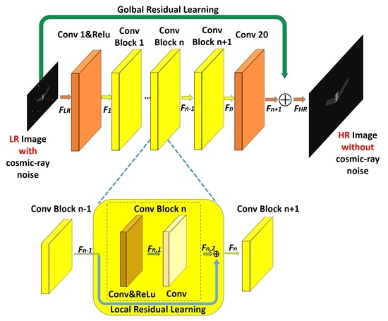
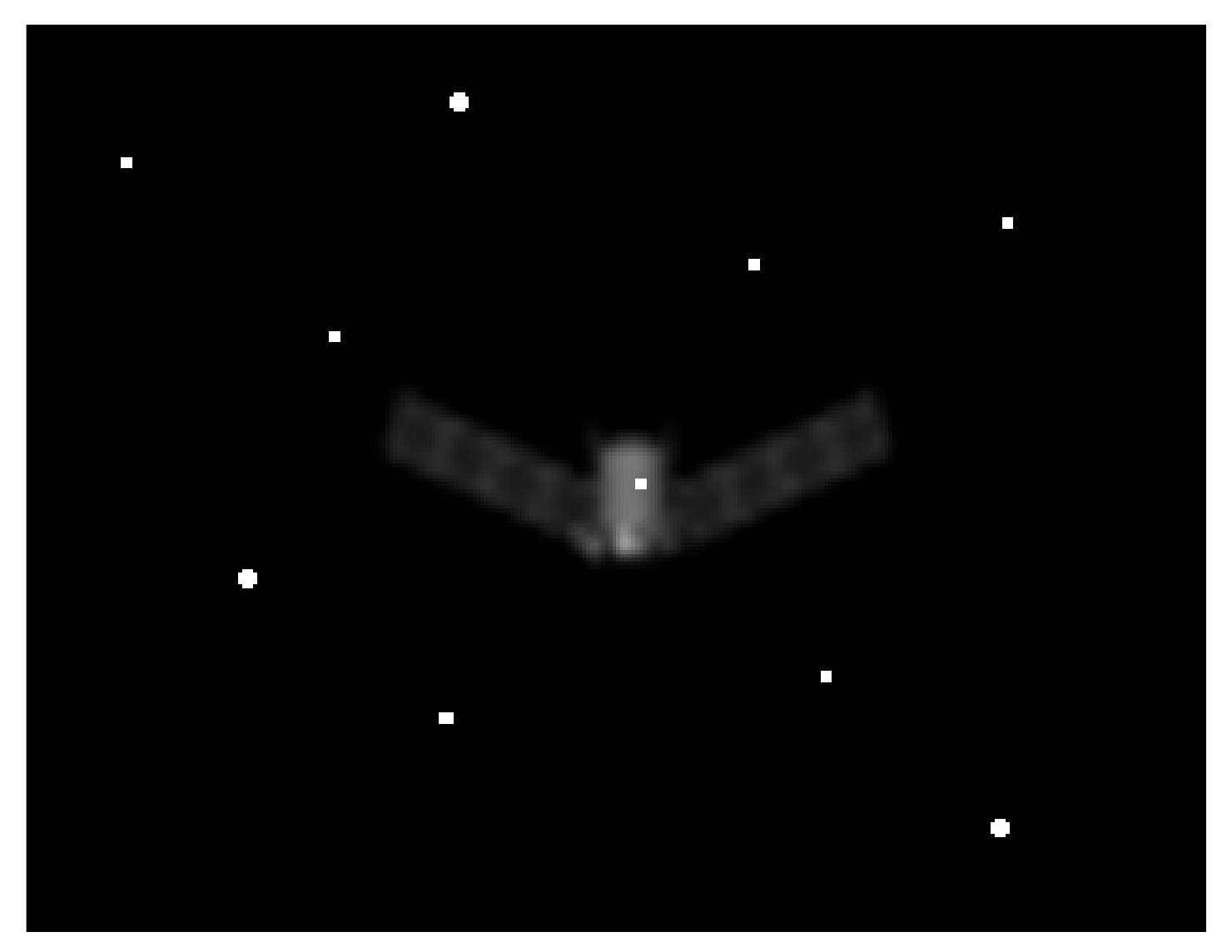
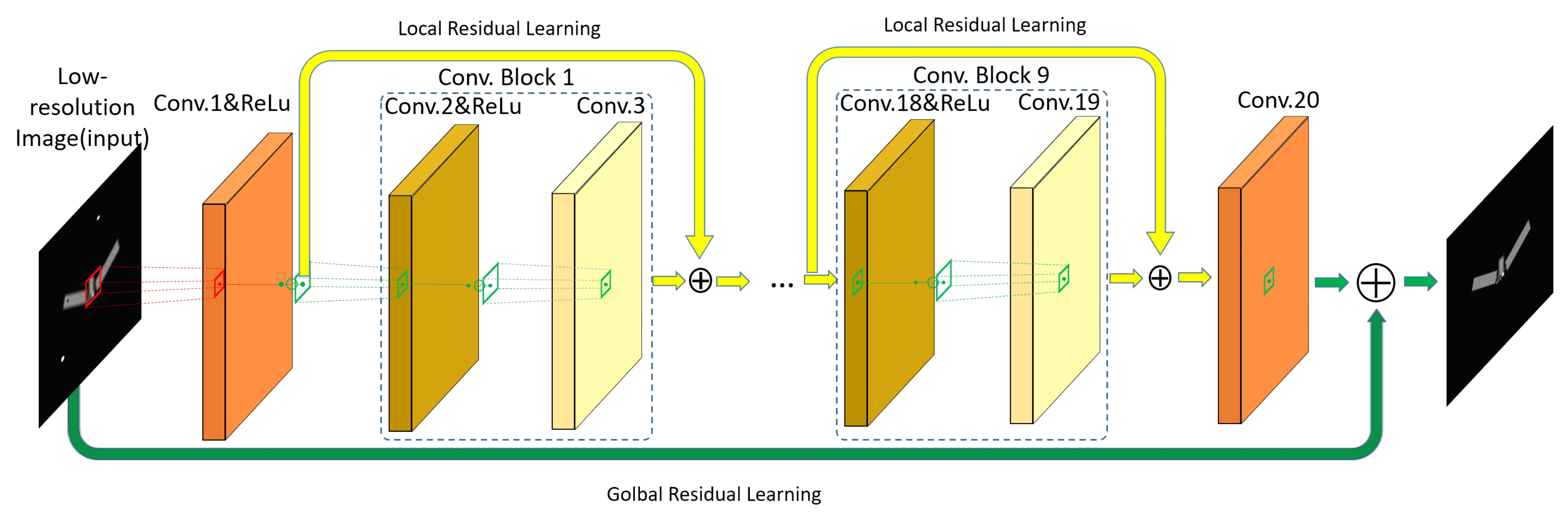
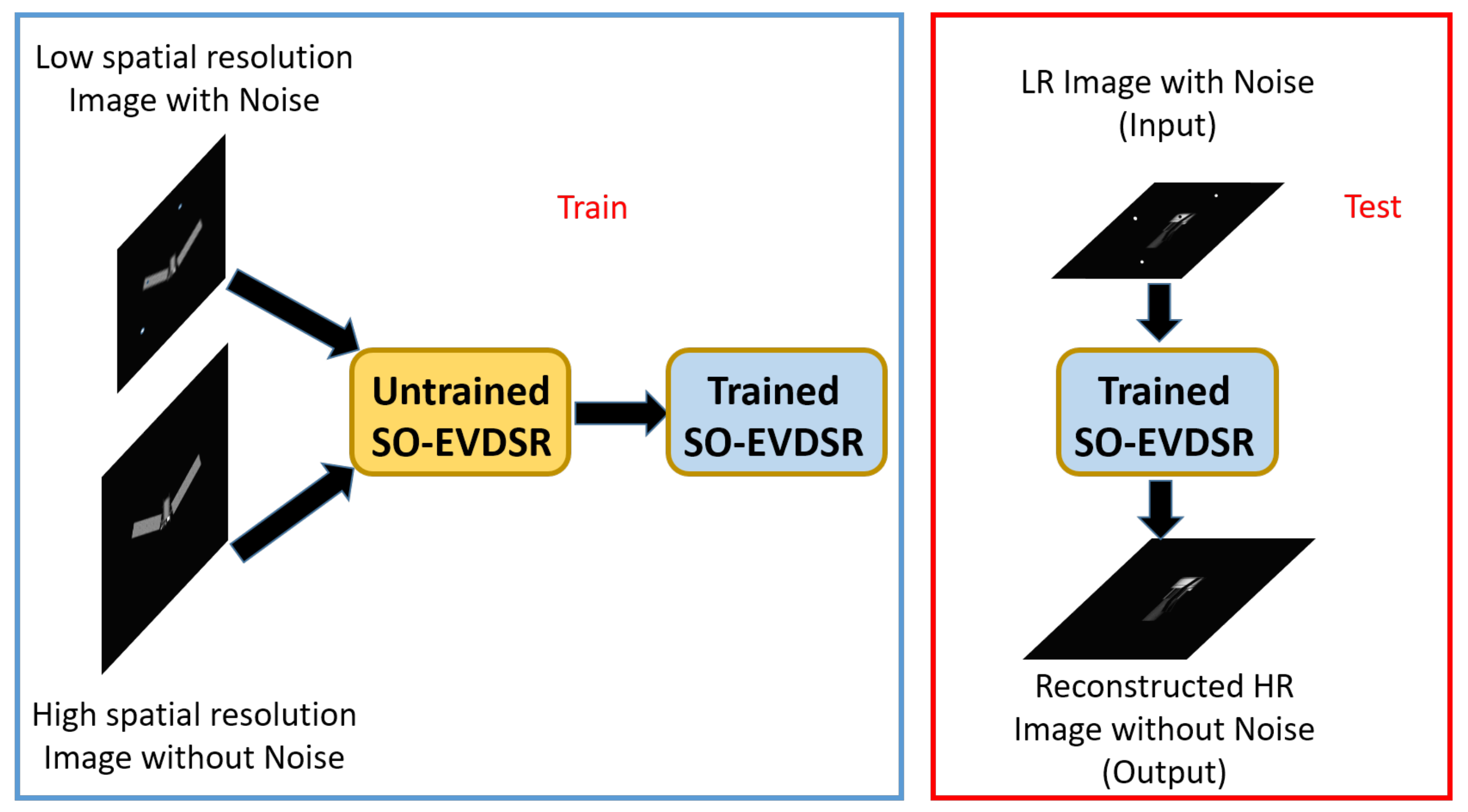
• We propose a method named SO-EVDSR. This method could remove cosmic-ray noise and enhance the spatial resolution of SO images in the meantime. It is the first time that a denoising and SR reconstruction method based on only one very deep convolutional network implemented in the SO images research field.
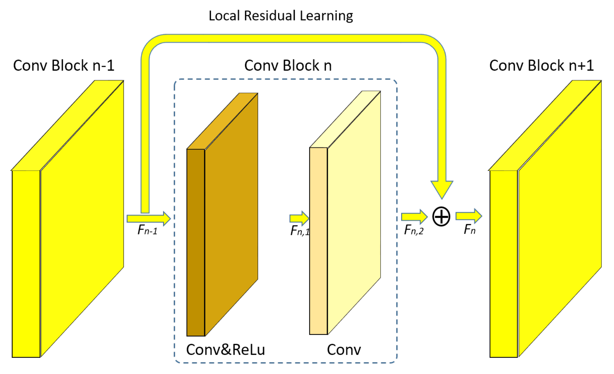
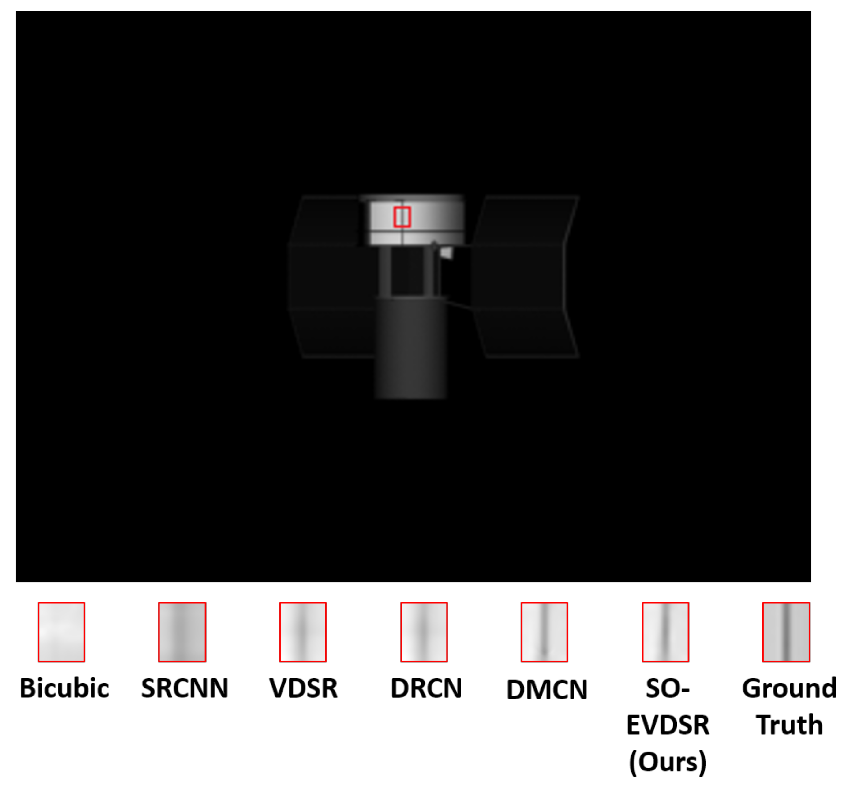
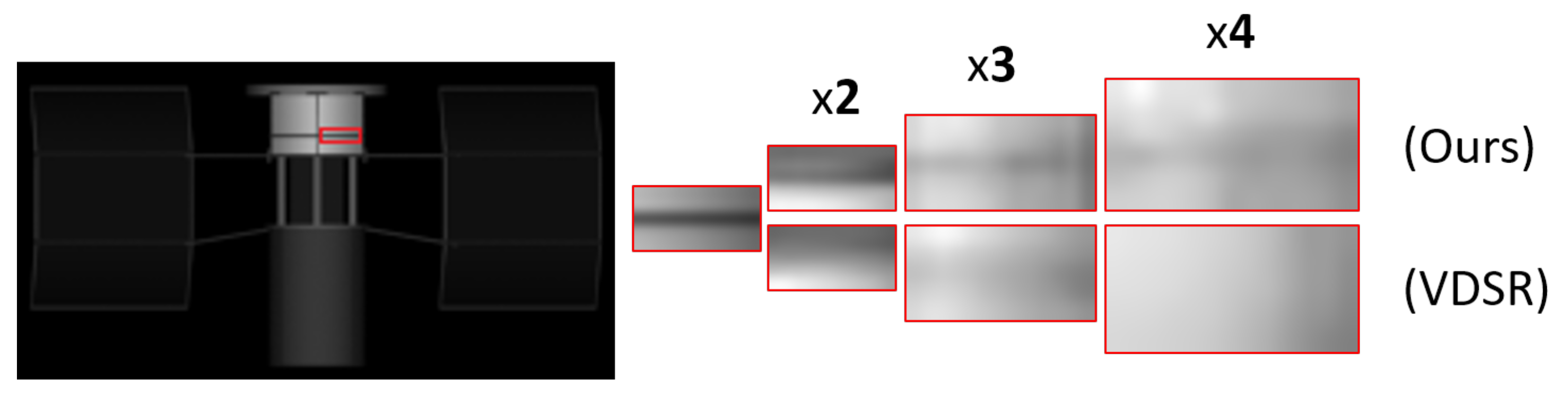
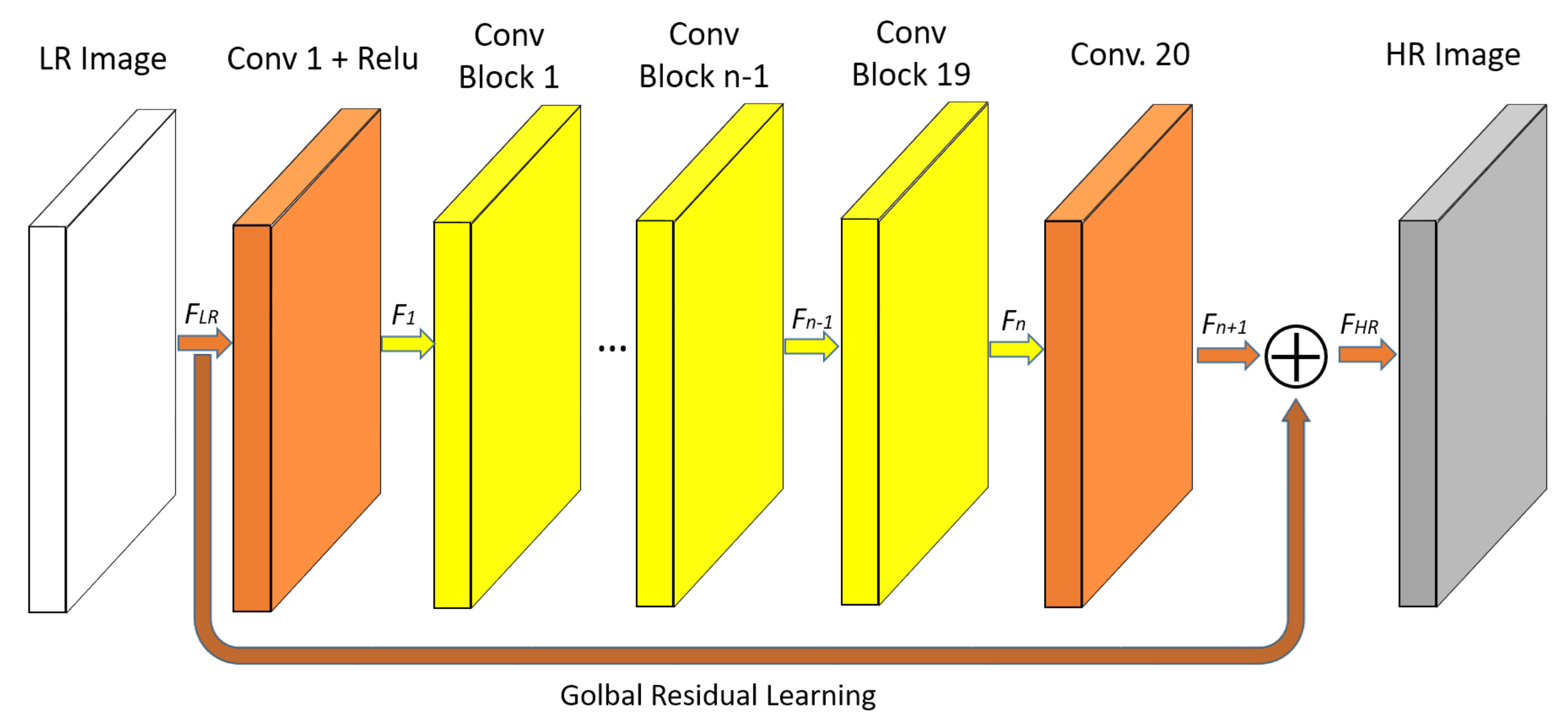
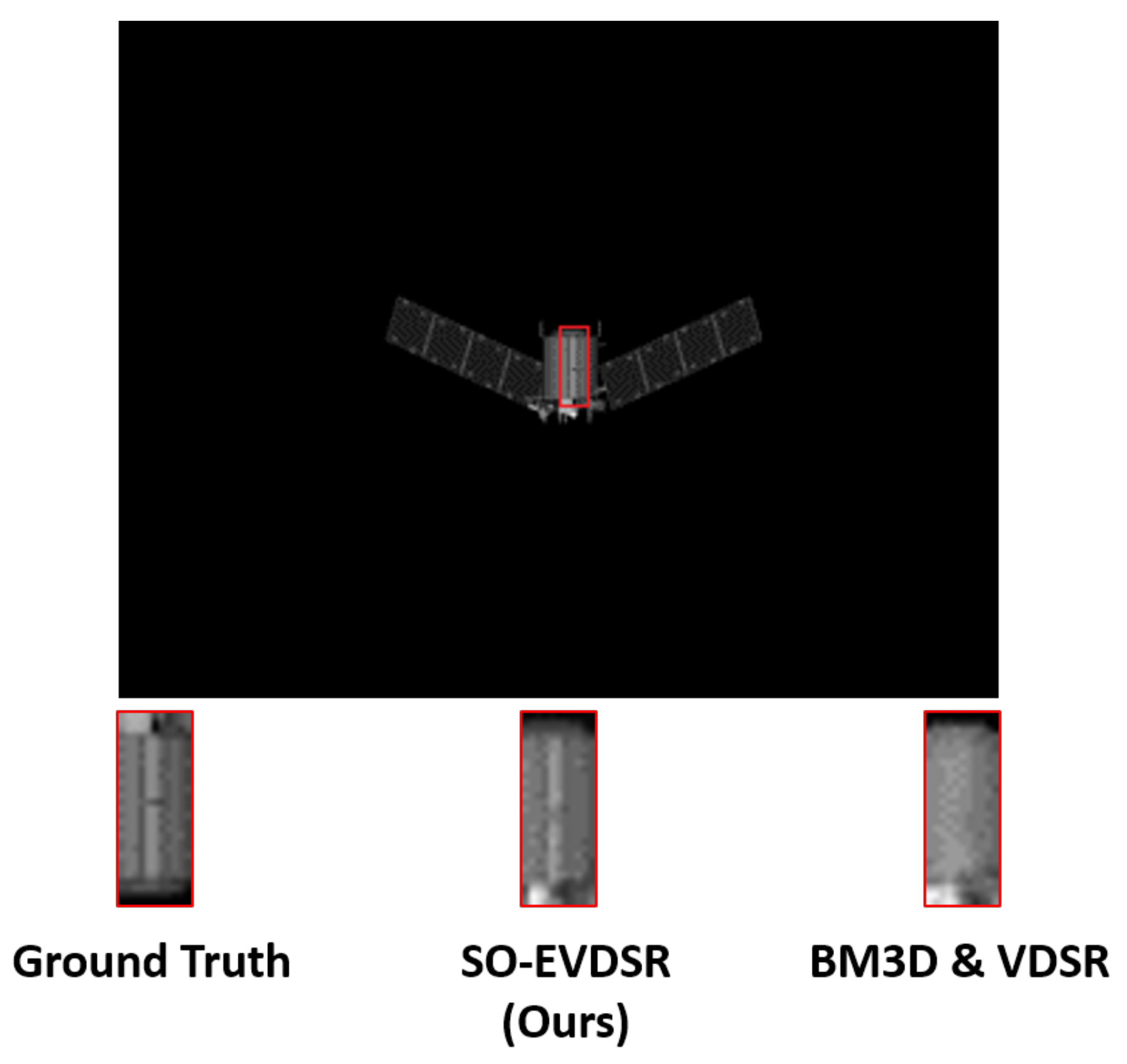
• This method combines the global residual learning and local residual learning. Experimental results show that our method performs better than several typical methods including some state-of-the-art methods in both quantitative measurements and visual effect.

The rest of this paper is organized as follows: in Section 2, we introduce and analyze some related works in denoising and solving SR problems, In Section 3, we give detailed descriptions of the proposed method. In Section 4, the detail of the experiment and the results are reported. In Section 5, some discussions are shown. Conclusion are drawn in Section 6.

2. Related Works

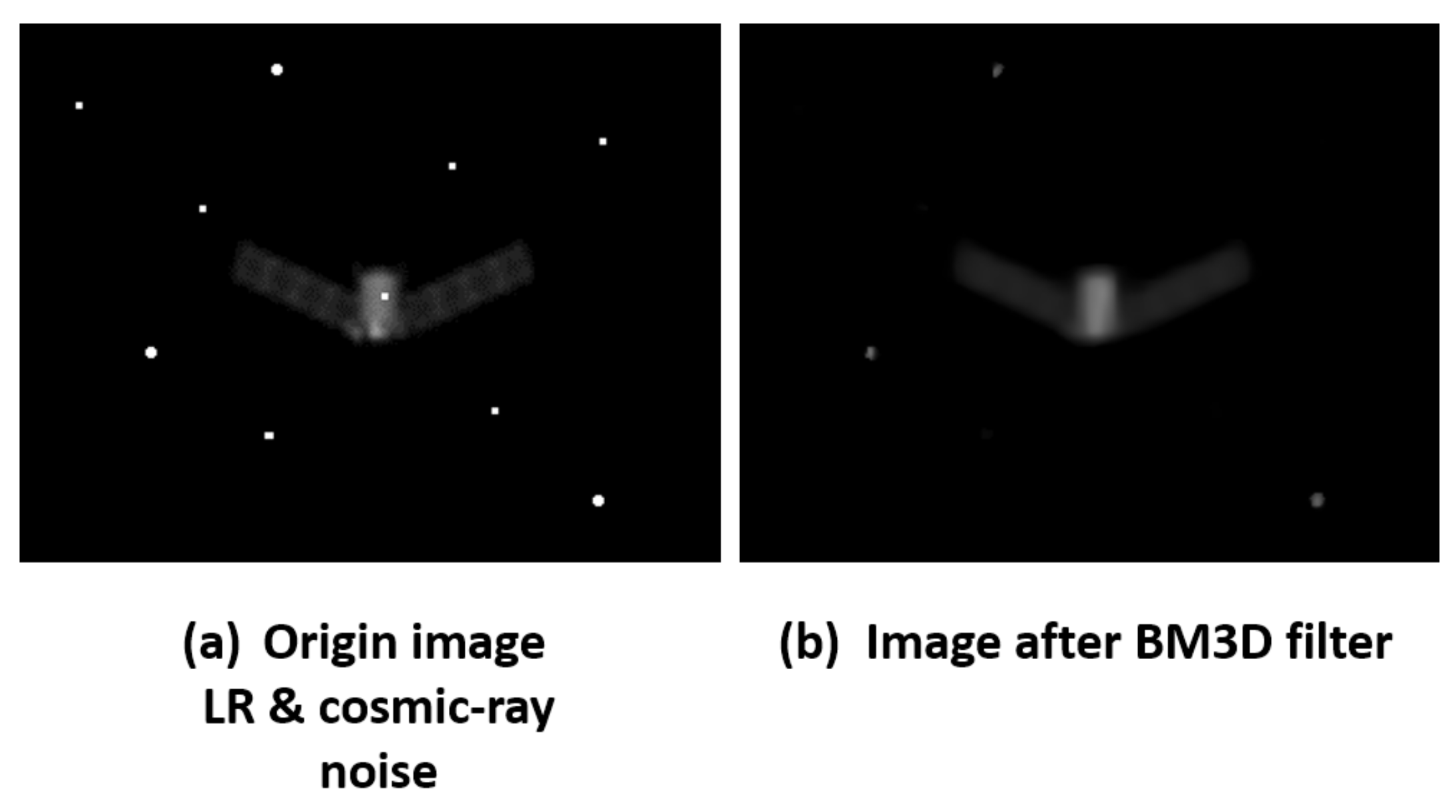
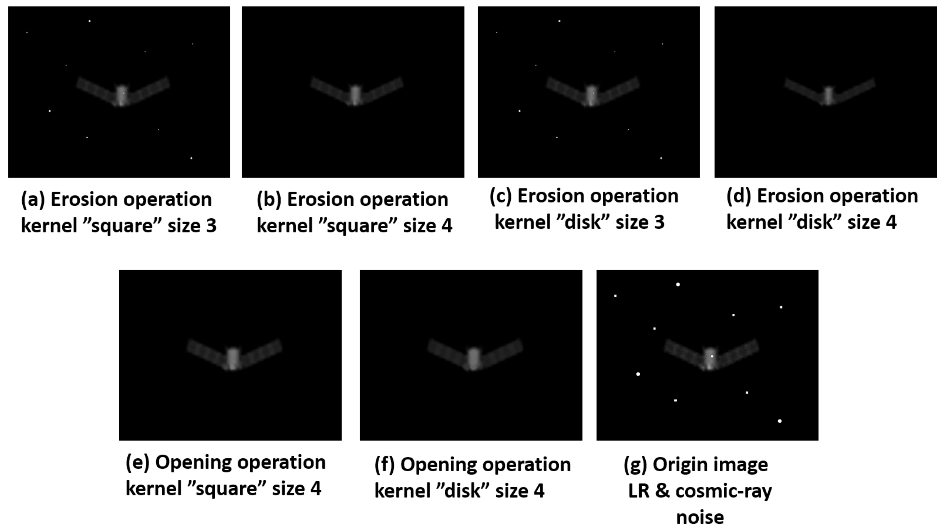
2.1. Cosmic-Ray and Denoising

As mentioned above, cosmic-ray noise could be regarded as salt and pepper noise, whose gray value is obviously higher or lower than surrounding pixels. But this type of noise is different from typical salt and pepper noise because its area is usually larger than one pixel, just like Figure 1 illustrated. The area whose gray value is obviously higher than surrounding pixels are cosmic-ray noise.

The early method to remove cosmic-ray noise in SO images is to take multiple images in the same field of view, just like Windhorst R.A. et al. [23] proposed. Then the cosmic-ray noise would be located based on sequential image information. Finally, a correct gray value is used to replace the gray value of the pixel contaminated by cosmic-ray noise. This type of method requires multiple images from the same field of view, which could not handle cosmic-ray noise in a single image.

Median filtering is one of the widely used classical methods to remove the cosmic-ray noise in a single SO image. But this method is no longer a very good method because it can further blur the edge of the SO image, which is not good for SR problem.

There are also some other conventional methods to remove the cosmic-ray noise in a single SO image. Zhu Z. et al. [24] first, make the first-order difference in two directions of the image, and the difference result is compared with the threshold to distinguish noise and candidate noise. Then, a Bessel curve fitting method is used to calculate the deviation of candidate noise. Finally, cosmic-ray noise is identified. The drawback is this model is that it is so simple that the applicability of this method is not good. Dokkum P.G. [25] uses a Laplacian edge detection method to detect cosmic-ray noise. This method achieves a very good effect in removing cosmic-ray noise. However, it does not consider the presence of bright supersaturated space objects. To reduce the running time, Pych. W. [26] proposed a fast removing cosmic-ray noise method based on image histogram. This method does not need to model objects, nor does it need a high signal-to-noise ratio. However, the drawback of this method is spectral energy in some pixels would be eliminated incorrectly.

Recently, CNN-based methods have achieved better results than conventional methods in the computer vision area [27,28]. So, some CNN-based denoising methods are appearing constant. Because cosmic-ray noise belongs to a type of salt and pepper noise, let us discuss some CNN-based denoising methods in removing salt and pepper noise.

The first CNN-based method to solve the denoising problem was proposed by Jain et al. [29]. This method achieved similar or even better results compared with other conventional methods. Mao et al. [30] proposed an auto-encoders with symmetric skip connections network. This method implemented 10 pairs of symmetrical convolutional and deconvolutional layers, whose first five layers are coding layer and the last five layers are decoding layer. From this method, the CNN-based network for image denoising became deeper and deeper. Zhang et al. [31] proposed DnCNN combined batch-normalization and residual learning and achieved state-of-the-art results.

2.2. Single Image Super-Resolution

Like the denoising problem, CNN-based methods are becoming more popular and efficient. Due to the limited space, we only discuss some works on the most representative CNN-based SISR reconstruction methods.

SRCNN is the first CNN-based SISR method, which achieved better results than conventional methods. It was proposed by Dong et al. [3,20] SRCNN is the first SISR method based on CNN, and discussed the relationship between SRCNN and the spare-coding method, which is one of the typical conventional SR methods. This method was then further improved mainly by increasing network depth or sharing network weights. SRCNN consists of three layers, which are inspired by sparse-coding: feature extraction, non-linear mapping, and reconstruction. Filters of spatial sizes $9\times 9$, $1\times 1$ and $5\times 5$ are used respectively. For validation, LR images are created by the downsampling of HR images, then are transformed through a HIS transform. The Intensity channel matrix is upscaled through the network. Finally, an HIS reverse transform is implemented to generate the final image.

VDSR [21] is the first CNN-based SISR method using residual learning. VDSR always consists of several layers, which could deepen the network. VDSR achieved very good results and became one of the state-of-the-art SISR methods. Normally, Kim et al. [21] uses a 20 layers network to train and test data in that paper. As the basic theory in VDSR, residual learning [22] is very important and affects many methods in deepening the convolutional network. Conventional convolutional networks or fully connected networks will more or less lose information when transmitting information. At the same time, gradient disappearance or gradient vanishment will cause deep networks hard to train. Residual learning could solve this problem. By directly transferring input information to output, the integrity of information is protected. The whole network only needs to learn the difference between input and output, which simplifies the learning goal and difficulty. So, the depth of the residual network is much deeper than the depth of conventional convolutional network.

DRCN [32] combines residual learning and recursive network and it was also proposed by Kim et al. for solving the SISR problem in the same year. DRCN is another CNN-based method, which combines residual learning and recursive neural network. This network takes an interpolated image as input and is divided into three modules. The first module is Embedding network, which could extract feature maps. This module is a recursive network. The second module is the inference network, which can do non-linear mapping. The last module is the reconstruction network, which could reconstruct the final result.

DMCN is another CNN-based method, which proposed by Xu et al. [33]. This method is used to handle various remote-sensing image restoration tasks such as SR and Gaussian denoising. This method also build local and global memory connections to combine image detail with global information. This method could not only solve SR problems but also achieve a very good denoised result.

3. Proposed Method

In this section, the problem definition is discussed first, then the details of our proposed method, SO-EVDSR, are given.

3.1. Problem Definition

Because of the lack of data in the remote-sensing area, a single image for denoising and super-resolution reconstruction is one of the best ways to solve this problem. So, our method could be defined as this: recover a HR image from its LR version. The relationship between HR image and its LR version could be achieved by the final trained output of the CNN-based network, which takes a lot of HR ground truth and its LR downsampling as inputs.

In summary, the purpose of solving the denoising and SISR problem using a CNN-based method is to establish a mapping F from the LR image to its HR reconstruction image, which is as similar as possible to the ground truth HR image. Let us denote the LR image as Y. Our goal is to recover from Y an image F(Y). In our proposed method, SO-EVDSR is the mapping F that could recover from Y an image F(Y).

By the way, image denoising problem and SR problem are similar because these two problems all need to be processed high-frequency parts while most other information preserved. Although the noise in obtained SO images is caused by cosmic-ray, it could still be regarded as a kind of salt and pepper noise. So only one deep CNN-based network is used to solve these two problems. That means there is only one mapping F in our method.

The training and testing procedure of our SO-EVDSR are illustrated in Figure 2. Pairs of LR images and HR images were sent to SO-EVDSR for training, then other LR images are sent to SO-EVDSR for testing.

3.2. Proposed Network

In this subsection, the structure of our SO-EVDSR is proposed first. Then the details of global residual learning and local residual learning in our method are also discussed.

3.2.1. Enhanced Very Deep Super-Resolution Network in Space Object Researching

The proposed SO-EVDSR is illustrated in Figure 3. SO-EVDSR takes an interpolated LR image (to the desired size) with simulated cosmic-ray noise (salt and pepper noise) as input. The HR image with noise well removed is reconstructed by SO-EVDSR.

SO-EVDSR is a very deep convolutional network that contains 20 convolutional layers. These convolutional layers were divided into three types. The first convolutional layer with relu belongs to the first type. The last convolutional layer without relu belongs to the second type, The rest belong to the third type, which includes nine identical convolutional blocks. Each convolutional block contains two convolutional layers with one relu. SO-EVDSR combines one global residual learning (GRL) and nine local residual learning (LRL). Except for the first and the last, the rest of layers are in the same type: 64 filters of the size $3\times 3\times 64$, where a filter handle on $3\times 3$ spatial region through 64 feature maps. The first layer handles the input image. The function of the last layer, which consists of a single filter of the size $3\times 3\times 64$, is reconstructing image.

By the way, our output image has the same size as the input image by padding zeros every layer during training.

The configuration of SO-EVDSR is shown in

Table 1. Enhanced very deep super-resolution network in space object researching (SO-EVDSR) configuration.

Block	Layer	Name	Conv<Receptive Field Size>-<Number of Channels>-<Number of Filter>	Parameters
	1	Conv	Conv3-1-64	1664
		Relu
1	2	Conv	Conv3-64-64	102,464
		Relu
	3	Conv	Conv3-64-64	102,464
2	4	Conv	Conv3-64-64	102,464
		Relu
	5	Conv	Conv3-64-64	102,464
3	6	Conv	Conv3-64-64	102,464
		Relu
	7	Conv	Conv3-64-64	102,464
4	8	Conv	Conv3-64-64	102,464
		Relu
	9	Conv	Conv3-64-64	102,464
5	10	Conv	Conv3-64-64	102,464
		Relu		102,464
	11	Conv	Conv3-64-64	102,464
6	12	Conv	Conv3-64-64	102,464
		Relu
	13	Conv	Conv3-64-64	102,464
7	14	Conv	Conv3-64-64	102,464
		Relu
	15	Conv	Conv3-64-64	102,464
8	16	Conv	Conv3-64-64	102,464
		Relu
	17	Conv	Conv3-64-64	102,464
9	18	Conv	Conv3-64-64	102,464
		Relu
	19	Conv	Conv3-64-64	102,464
	20	Conv	Conv3-1-64	102,464

.

3.2.2. Residual Learning in SO-EVDSR

Residual learning means the input and output are largely similar, so in our method, a residual $r=y-x$ is defined, where most values are likely to be zero or small. Using residual learning to solve SR problems had been demonstrated in a very effective way [21]. In SO-EVDSR, r is the residual pixel of x and y. So, we could make the whole network training easy and could further make the whole network deeper than normal. It could roughly be divided into two types, i.e., global residual learning and local residual learning.

Global residual learning. The global residual learning (GRL) in SO-EVDSR is a long skip connection that could make the whole network deeper and easier to train. As illustrated in Figure 4, it usually connected the input and the output of the last convolutional layer by the Equation (1).

$$F_{HR}=F_{LR}+F_{n+1}.$$

(1)

$F_{HR}$, $F_{LR}$ and $F_{n+1}$ denote the global residual learning of mapping F whose function is reconstructing the final result, the input image and the last convolutional layer of mapping F respectively.

Local residual learning. The local residual learning (LRL) was used to alleviate the degradation problem caused by ever-increasing network depths and improve the learning ability. It could further improve the information flow [34]. As illustrated in Figure 5, the Equation (2) could describe how LRL in our SO-EVDSR works.

$$F_n=F_{n,2}+F_{n-1}.$$

(2)

$F_n$, $F_{n,2}$ and $F_{n-1}$ denote the nth local residual learning of mapping F, the second convolutional layer of the n-th convolutional block and the $(n-1)$-th local residual learning of mapping F.

4. Experiment

In this section, the dataset we used in this article is discussed first. Then training parameters we used are discussed and given the final parameters we used. The experimental results are given in the last part of this section.

4.1. Dataset

The dataset this paper used was BUAA-SID1.0 [35], which contains 9200 gray images of the size $320\times 240$. Before this dataset is established, there were no public documents about SO and image simulation mentioned SO image database, which contained abundant geometric characteristics. But the geometric characteristics of SO are very important for detecting and recognizing. Therefore, this database, which contains different viewing angles of 20 satellites, has great significance. The names of satellites in the database are a2100, astrolink, cobe, dsp, early-bird, eo1, ers, esat, ets8, fengyun, gallieo, glonas, goms, helios2, irns, is-601, minisat-1, radarsat-2, timed and worldview, respectively.

We separated the whole database into a training set and testing set with a hold-out method. We used 80% to train and 20% to test, because in SO research field, images obtained are comparatively similar and the requirements of reconstruction precision are higher than those of normal image (like cat or dog). First, we randomly chose 16 satellites (7360 images) as a training set and the other four satellites (1840 images) as a testing set. In order to shorten the experiment time, we randomly chose 20 images of different satellite attitudes from each satellite in the training set we mentioned above. Similarly, we also chose 20 images of different satellite attitudes from each satellite in the testing set. All images used in our experiment were down-sampled into 1/2, 3/1 and 1/4, respectively. Then salt and pepper noise was added to these down-sampling images. This could be used to simulate the actual situation. Finally, all images were separated into pieces of the size $41\times 41$.

4.2. Training Parameters

We now describe some details of our training model. Let Y denote an interpolated LR image and X a HR image. A training dataset ${\left\{x^{\left(i\right)},y^{\left(i\right)}\right\}}_{i=i}^N$ was given, and our goal was to learn an end-to-end relationship model F that predicts values $\widehat{X}=F\left(X\right)$, where $\widehat{X}$ is the prediction from LR image. We used mean squared error and L2 regularization to train the parameters. The definition of L2 loss function was illustrated in Equation (3):

$$L_2=\frac{1}{2M}\sum _i^M\sum _j^M{\left(F\left(Y_{ij}\right)-X_{ij}\right)}^2$$

(3)

As illustrated in Equation (3), M represents the number of samples, $F\left(Y\right)$ represents reconstructed image, and X represents the ground truth.

Depth. The depth of the network is a very important parameter. In VDSR [21], the author has verified the training results of the network from five layers to 20 layers. The results show that when the network layers are 20, the best result can be achieved by considering the training time and training effect comprehensively. We verify this conclusion, and the results are consistent with VDSR. As Figure 6 shows, we further deepened the network to 25 layers and found that the Peak Signal-to-Noise Ratio (PSNR) was not significantly enhanced. So we use 20 layers to train and test.

Learning rate. One possible reason that could affect the convergence of the model is learning rate. A basic rule of learning rate is that a high learning rate could boost training. But simply setting the learning rate higher could also lead to vanishing or exploding gradients, which could make the whole network difficult to converge.

Figure 7 illustrates the comparing result of different initial learning rates. This result shows that the learning rate was very important for training and only a proper learning rate could achieve the best effect.

Gradient clipping. Gradient clipping is used in our training. In essence, the chain derivative was used in the back-propagation method while training. When calculating the gradient of each layer, some multiplication operations will be involved. Therefore, if the network was too deep, most of the multiplication factors were greater than unity, then the final result may tend to be infinite, which is called gradient exploding. Gradient clipping is a method that is often used to resolve gradient exploding problem. By setting a threshold $\theta$, the gradient will be limited to that range $\left[-\theta ,\theta \right]$ when it exceeds to the threshold.

Mini-batch gradient descent. Mini-batch gradient descent is a compromise method between the batch gradient descent method and the stochastic gradient descent method. This method not only ensures the accuracy, but also speeds up the convergence. So, this method was also used in our training.

Epochs. Epoch is another important parameter in training. Figure 8 illustrate the result of increasing epoch. The result shows that peak signal-to-noise ratio did not increase obviously after 120 epochs.

Finally, we used a network of depth 20. Momentum and weight decay parameters are set to 0.9 and 0.001, respectively. Training batches were set to 64. We trained our model over 120 epoch. The learning rate was initially set to 0.001 and then decreased by a factor of 10 every 20 epochs. We used NVIDIA Tesla P4 to run our experiment and the total time taken by training was almost eight hours.

4.3. Results

To evaluate the result of these algorithms, we used quantitative measures to compare these results. Normally, we use five methods to evaluate the results.

4.3.1. Quantitative Measurements

PSNR is the most commonly used measurement to evaluate the result of an image. It is defined as the ratio between the maximum possible value of a signal and the value of distorting noise that affects the quality of its representation [36]. The definition of PSNR is showed in Equation (4):

$$PSNR=10{log}_{10}\frac{{\left(maximumpixelvalue\right)}^2}{MSE}$$

(4)

The MSE witch is defined in Equation (5) is the mean square error. X and $F\left(Y\right)$ are the ground truth and reconstructed image, respectively. M and N are number of rows and columns in the images X and $F\left(Y\right)$, respectively.

$$MSE=\frac{{\sum }_{j=1}^N\left({\sum }_{i=1}^M{\left(F\left(Y_{i,j}\right)-X_{i,j}\right)}^2\right)}{MN}$$

(5)

$$SSIM=\frac{\left(2{\mu }_x{\mu }_y+C_1\right)\left(2{\sigma }_{xy}+C_2\right)}{\left({\mu }_x^2{\mu }_y^2+C_1\right)({\sigma }_x^2+{\sigma }_y^2+C_2))}.$$

(6)

Another most commonly used measurement is the structure similarity (SSIM), which is defined in Equation (6). In Equation (6), a and b refer to images X and $F\left(Y\right)$, which are referenced the ground truth and the reconstructed HR image respectively. $C_1$ and $C_2$ are constants. ${\mu }_x$ is the local mean of reference (X) image and ${\mu }_y$ is the local mean of the reconstructed $F\left(Y\right)$ image. ${\sigma }_x$ and ${\sigma }_y$ are the standard deviations and ${\sigma }_{xy}$ is the cross-covariance for these images. Finally, a higher SSIM is better.

However, in this article, SSIM was probably not a good metric as the numbers were so close in different methods up to the fifth or sixth decimal places (as illustrated in

Table 2. Results of applying the SR methods to the BUAA-SID1.0 image.

Method	Scale	MSE	PSNR	SSIM	HVS	HVSm
Bicubic	2	4.810885296	41.30855358585935	0.9999984940625836	54.1835	54.2532
	3	9.004434909	38.58623897872875	0.9999963947901308	52.2901	52.3281
	4	13.07634938	36.96593844957169	0.9999929499766917	50.8295	51.0292
SRCNN	2	3.087851266	43.23423987529352	0.9999989854654752	56.5810	56.7858
	3	6.815264731	39.79597630702207	0.9999972759376027	54.6213	54.9024
	4	10.10653004	38.08478289567298	0.9999954949789307	52.0198	52.2285
VDSR	2	2.518198065	44.11990474992009	0.9999992553686302	57.0211	57.2354
	3	5.540032111	40.69568078908413	0.9999982028334025	55.2018	55.3811
	4	8.284960877	38.94789898927323	0.9999968440793972	52.7028	53.0285
DRCN	2	2.452489995	44.23473116546864	0.9999992569876331	57.8302	58.0522
	3	5.527730285	40.70533516546694	0.9999982135434648	56.0238	57.2419
	4	8.263899739	38.95895321354315	0.9999968452134436	53.5229	53.9219
DMCN	2	2.370692141	44.38205200938572	0.9999992858920935	59.3410	60.1925
	3	5.31803133	40.87329469327502	0.9999982947593297	56.6815	58.2859
	4	8.124998092	39.03257093209752	0.9999969012845702	54.0283	54.8921
SO-EVDSR	2	2.263607982	44.58279144085883	0.9999993199209739	61.4168	62.0269
	3	5.08946923	41.06407867788109	0.9999983700995432	59.0214	60.1920
	4	7.891428243	39.15924749054321	0.9999969575852177	57.1832	57.9237

). So the human visual system (HVS) [37] and human visual system model (HVSm) [37] metrics are also used to compare the reconstruction performance among different methods.

The HVS metric is defined as Equation (7).

$$HVS=20log(255/MS{E}_H).$$

(7)

In Equation (7), $MS{E}_H$ is defined as Equation (8).

$$MS{E}_H=K\sum _{i=1}^{M-7}\sum _{j=1}^{N-7}\sum _{m=1}^8\sum _{n=1}^8{((D{[m,n]}_{i,j}-D{[m,n]}_{i,j}^e)Tc[m,n])}^2$$

(8)

In Equation (8), M and N denote image size respectively, $D_{ij}$ denotes the Discrete Cosine Transform (DCT) [38] coefficients of $8\times 8$ image block for which the coordinates of its upper left corner are equal to i and, $D{e}_{ij}$ denote the DCT coefficients of the corresponding block in the original image and K denotes $1/\left[\right(M-7\left)\right(N-7\left)64\right]$. Finally, $Tc$ denotes the matrix of correcting factors which was introduced in [39].

The only difference between HVS and HVSm is the visual masking effects are taken into account by HVSm. First, DCT coefficients of size $8\times 8$ original image block and $8\times 8$ processed image block are calculated between pixel values, then a reduction based on the value of contrast masking was done. Finally, we calculated $MS{E}_H$. More details could be found in [40].

4.3.2. Quantitative Results

Table 2 shows that based on BUAA-SID1.0 dataset, our SO-EVDSR model has the best performance (red text in Table 2) in MSE, PSNR, SSIM, HVS and HVSm.

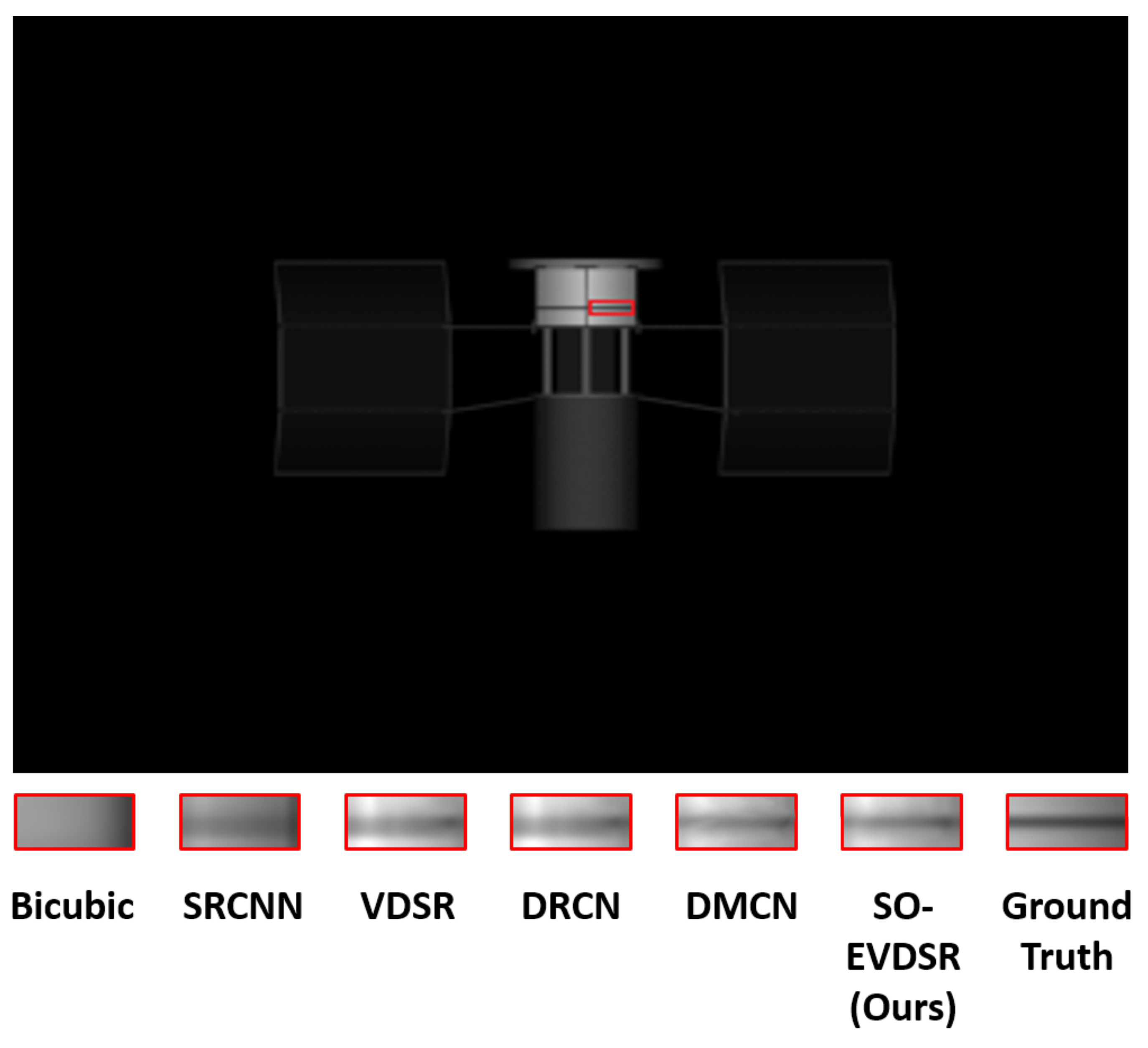
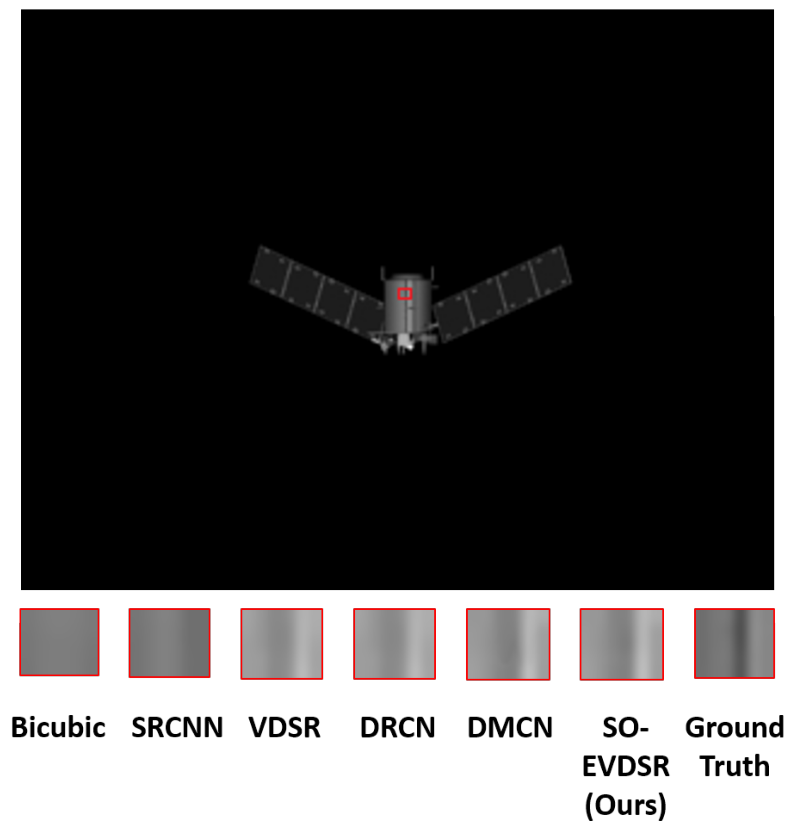
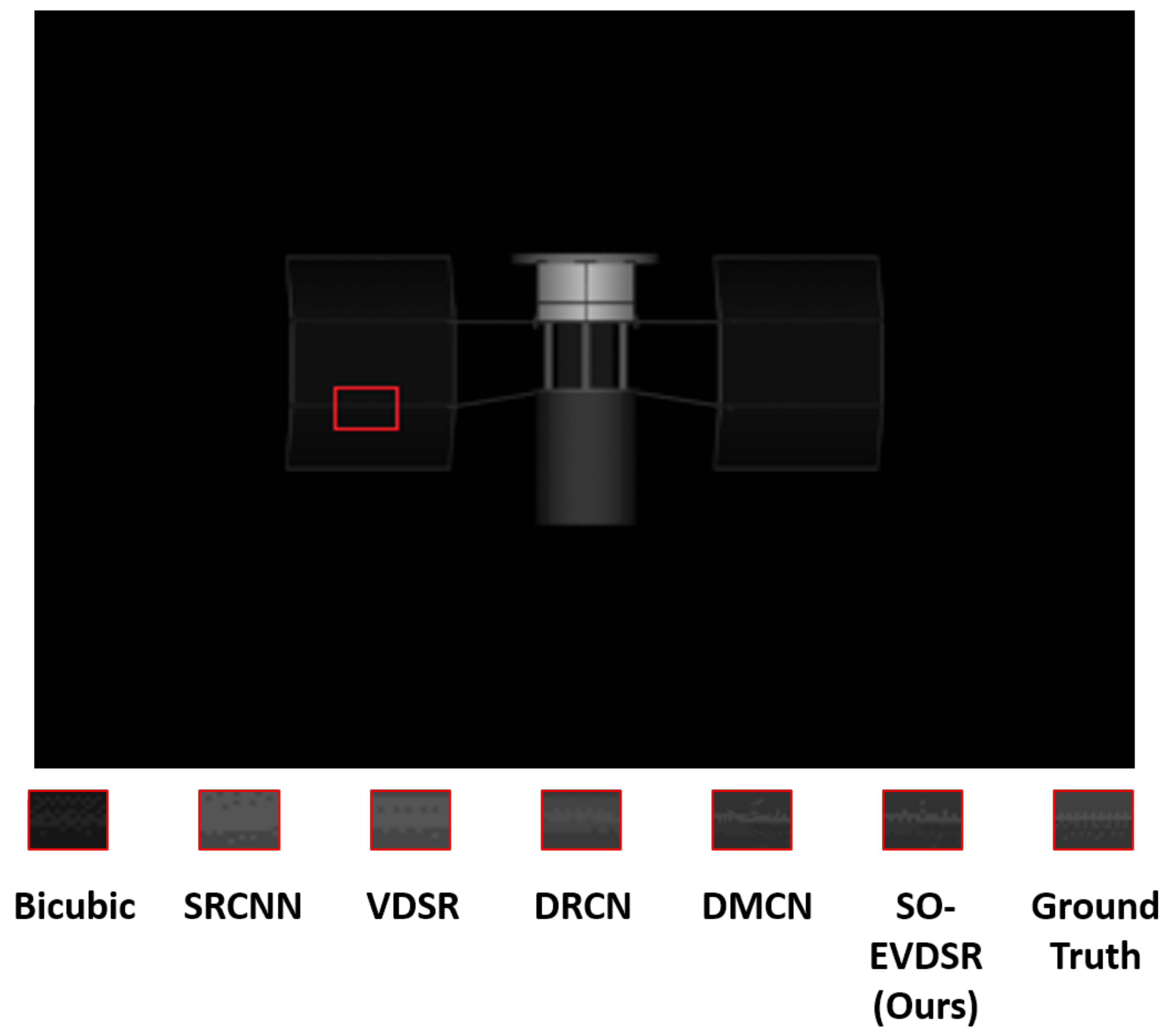
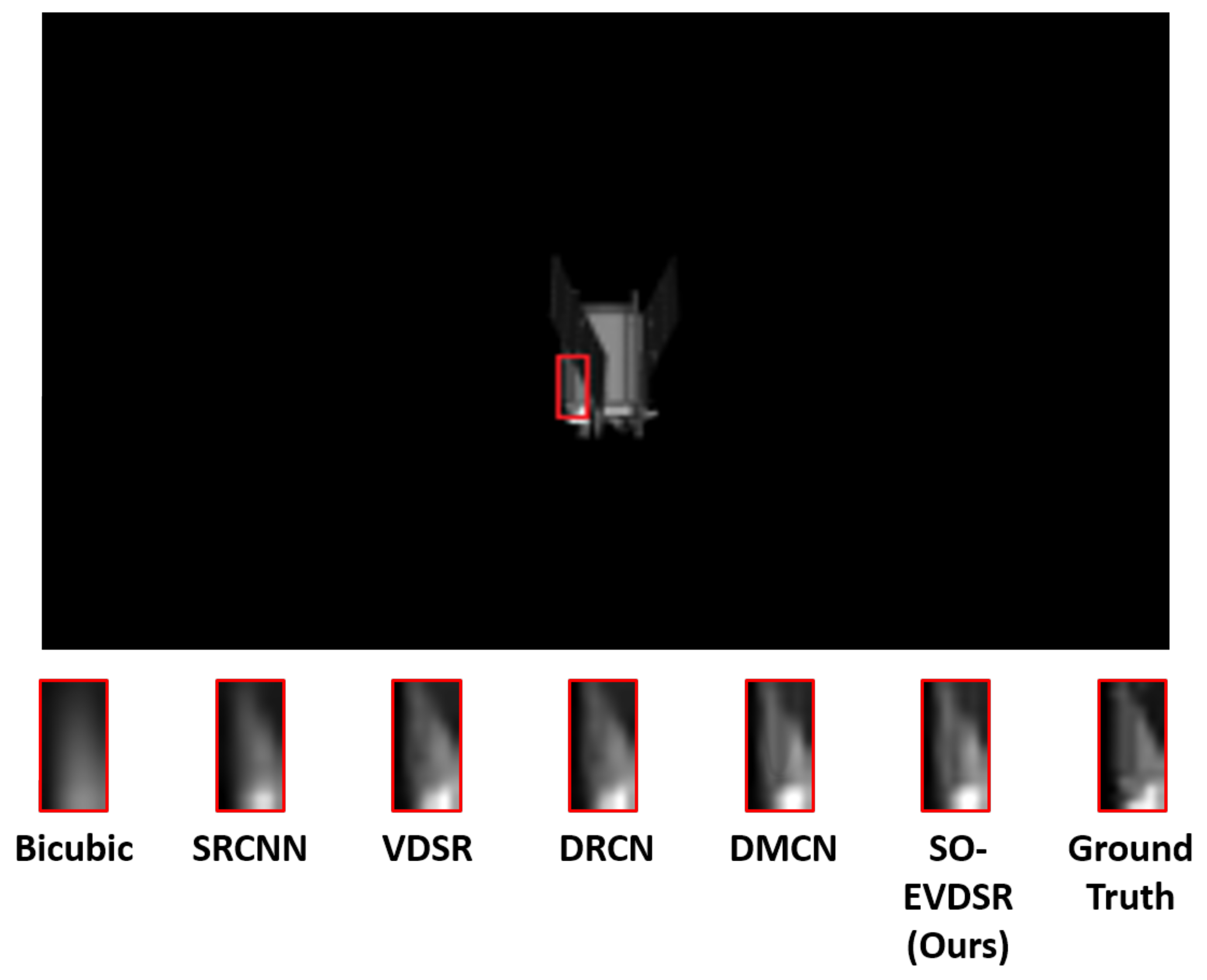
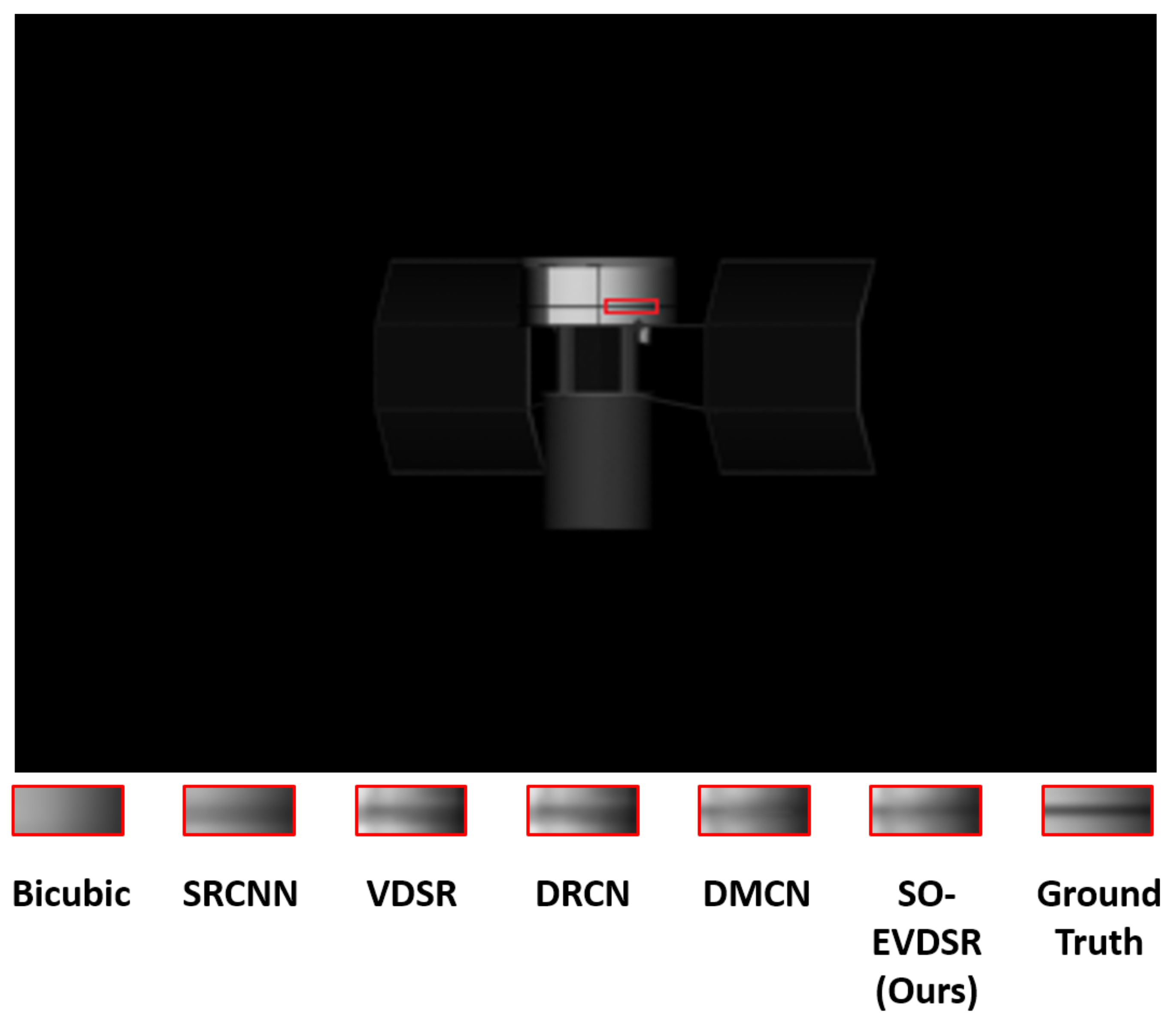
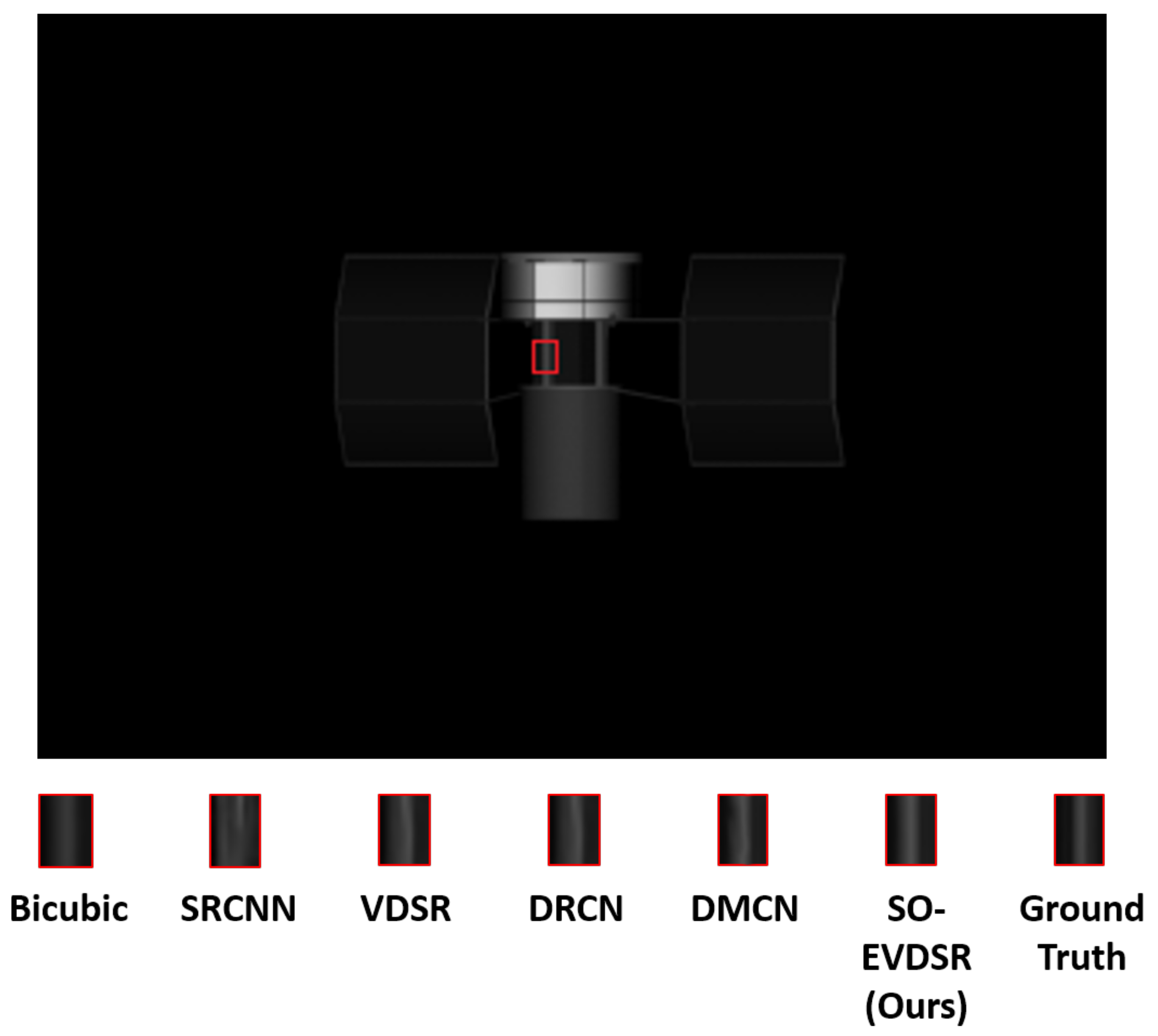
4.3.3. Visual Comparison Results

Firstly, we applied some classical methods to deal with cosmic-ray noise. Figure 9 shows the result of median filtering with filter sizes $3\times 3$, $5\times 5$, $7\times 7$ and $9\times 9$. The result shows that filter size $3\times 3$ and $5\times 5$ could not remove cosmic-ray noise completely, while $7\times 7$ and $9\times 9$ could remove cosmic-ray noise, but also cause further loss of image details. Therefore, using median filtering only could not achieve ideal denoising effect, and it is not suitable for space object image processing because of the high-precision measurement.

Then, Figure 10 shows the result of using an erosion operation to deal with cosmic-ray noise. We used the “disk” and “square” kernel type respectively. The result shows that when the kernel size was 3, cosmic-ray noise could not be removed, and when the size was 4, cosmic-ray noise could be removed, but at the same time, the satellite details were obviously lost, so the simple erosion operation could not achieve the desired denoising effect. Then the expansion operation of the same size was added, the combination of these two operations was called the opening operation. The results show that the image details will still be lost further. Therefore, only using the erosion operation or opening operation could not achieve ideal denoising effect, and it was not suitable for space object image processing because of the high-precision measurement.

Figure 11 shows the result of using the BM3D algorithm [41] to deal with cosmic-ray noise. The result shows that the ideal denoising effort is still not achieved and the image is blurred further. That is because BM3D could not regard cosmic-ray noise as typical noise, which it could deal with. The similar result happens on the algorithm, which was proposed in [42].

Visually, in Figure 12, Figure 13, Figure 14, Figure 15, Figure 16, Figure 17, Figure 18 and Figure 19, we could see the difference and enhancement among bicubic, SRCNN [3,20], VDSR [21], DRCN [32], SO-EVDSR, DMCN and the ground truth. We could also see the details that SO-EVDSR reconstructed, which SRCNN, VDSR, DRCN and DMCN could not reconstruct that clearly.

Compared to VDSR, which also could provide three scale factors in one network, our method not only performed better in scale factor 2, but also performed better in scale factor 3 and factor 4. Figure 20 shows the result of the comparison.

Finally, we also experimented using SO-EVDSR to compare with a cascade method, which applied a BM3D filter first to deal with cosmic-ray noise, then VDSR is applied to solve the SR problem. Figure 21 is the result of comparison and the result shows that the performance of the cascade method we applied was not as good as SO-EVDSR.

5. Discussion

Our SO-EVDSR, which combines GRL and LRL, achieves a very good result.

Table 3. Results of applying the SR methods to the BUAA-SID1.0 image.

Method	Scale	PSNR
Only Using GRL(VDSR)	2	44.11990474992009
	3	40.69568078908413
	4	38.94789898927323
Only Using LRL	2	44.00266113315757
	3	40.42742178926535
	4	38.63971533159192
SO-EVDSR	2	44.58279144085883
	3	41.06407867788109
	4	39.15924749054321

shows that based on the same training parameters, the combination of GRL and LRL has better performance in PSNR than using GRL or LRL only. This is different from Table 2. Table 2 focuses on comparing the effects of each single-frame super-resolution reconstruction method, while Table 3 is based on SO-EVDSR, comparing the effects of using GRL only (like VDSR), using LRL only and using GRL and LRL (like our method) at the same time. The result shows that our SO-EVDSR has the best performance in PSNR (red text in Table 3).

In this work, we show that a single space object image denoising and super-resolution problem could be well solved by a deep CNN-based method. This is the first time using CNN-based method to solve single SO image denoising and SR problem. The experiment result shows that cosmic-ray noise are well removed and textures, especially linear textures in a high-resolution image are recovered. However, future research needs to especially evaluate the improvement for images of a star, which is another important type of SO. The texture and detail in star images are very different from these in satellite images.

It also of interest to research residual learning. Because we have already seen that the effect of combining global residual learning and local residual learning. So, future research will try more combinatorial approaches of the two.

6. Conclusions

In this work, we have presented a CNN-based denoising and single-image super-resolution method named SO-EVDSR. This is the first time using a very deep CNN-based denoising and SISR method to reconstruct high quality SO images. We combine global residual learning and local residual learning to enhance the reconstruction effect. We have demonstrated that based on BAUU-SID1.0 dataset, which is a collection of satellite images affiliated to 20 satellites, our proposed SO-EVDSR not only could remove the cosmic-ray noise, but also has better performance than VDSR and DRCN do, which are two of the state-of-the-art SISR methods, in both quantitative measurements and visual effect.

References

1. He, Z.; Liu, L. Hyperspectral Image Super-Resolution Inspired by Deep Laplacian Pyramid Network. Remote Sens. 2018, 10, 1939. [Google Scholar] [CrossRef]
2. Pouliot, D.; Latifovic, R.; Pasher, J.; Duffe, J. Landsat Super-Resolution Enhancement Using Convolution Neural Networks and Sentinel-2 for Training. Remote Sens. 2018, 10, 394. [Google Scholar] [CrossRef]
3. Dong, C.; Loy, C.; He, K.; Tang, X. Learning a deep convolutional network for image super-resolution. In Proceedings of the European Conference on Computer Vision, Zurich, Switzerland, 6–12 September 2014; pp. 184–199. [Google Scholar]
4. Hou, H.; Andrews, H. Cubic spline for image interpolation and digital filtering. IEEE Trans. Image Process. 1978, 26, 508–517. [Google Scholar]
5. Dodgson, N. Quadratic interpolation for image resampling. IEEE Trans. Image Process. 1997, 6, 1322–1326. [Google Scholar] [CrossRef] [PubMed]
6. Huang, T.; Tsai, R. Multi-frame image restoration and registration. Adv. Comput. Vis. Image Process. 1984, 1, 317–339. [Google Scholar]
7. Kim, S.; Bose, N.; Valenauela, H. Recursive reconstruction of high resolution image from noisy undersampled multiframes. IEEE Trans. Acoust. Speech Signal Process. 1990, 38, 1013–1027. [Google Scholar] [CrossRef]
8. Hayat, K. Super-Resolution via Deep Learning. arXiv 2017, arXiv:1706.09077. [Google Scholar]
9. Timofte, R.; Rothe, R.; Gool, L.V. Seven ways to Improve Example-based Single Image Super-Resolution. In Proceedings of the IEEE Conference on Computer Vision and Pattern Recognition, Las Vegas, NV, USA, 26 June–1 July 2016; pp. 1865–1873. [Google Scholar]
10. Yang, J.; Wright, J.; Huang, T.S.; Ma, Y. Image super resolution via sparse representation. IEEE Trans. Image Process. 2010, 19, 2861–2873. [Google Scholar] [CrossRef] [PubMed]
11. LeCun, Y.; Bengio, Y.; Hinton, G. Deep learning. Nature 2015, 521, 436–444. [Google Scholar] [CrossRef] [PubMed]
12. Huang, G.; Zhuang, L.; Maaten, L. Densely Connected Convolutional Networks. In Proceedings of the IEEE Conference on Computer Vision and Pattern Recognition, Honolulu, HI, USA, 21–26 July 2017; pp. 4700–4708. [Google Scholar]
13. Simonyan, K.; Zisserman, A. Very deep convolutional networks for large-scale image recognition. arXiv 2015, arXiv:1409.1556. [Google Scholar]
14. Tong, T.; Li, G.; Liu, X.; Gao, Q. Image Super-Resolution Using Dense Skip Connections. In Proceedings of the IEEE International Conference on Computer Vision, Venice, Italy, 22–29 October 2017; pp. 4799–4807. [Google Scholar]
15. Mei, S.; Lin, X.; Ji, J.; Zhang, Y.; Wan, S.; Du, Q. Hyperspectral Image Spatial Super-Resolution via 3D Full Convolutional Neural Network. Remote Sens. 2017, 9, 1139. [Google Scholar] [CrossRef]
16. Zhang, K.; Zuo, W.; Zhang, L. Learning a single convolutional super-resolution network for multiple degradations. In Proceedings of the IEEE Conference on Computer Vision and Pattern Recognition, Salt Lake City, UT, USA, 18–22 June 2018; pp. 3262–3271. [Google Scholar]
17. Huang, J.; Singh, A.; Ahuja, N. Single image super resolution from transformed self-exemplars. In Proceedings of the IEEE Conference on Computer Vision and Pattern Recognition, Boston, MA, USA, 7–12 June 2015; pp. 5197–5206. [Google Scholar]
18. Kim, K.; Kwon, Y. Single-image super-resolution using sparse regression and natural image prior. IEEE Trans. Pattern Anal. Mach. Intell. 2010, 32, 1127–1133. [Google Scholar] [PubMed]
19. Jiang, K.; Wang, Z.; Yi, P.; Jiang, J.; Xiao, J.; Yao, Y. Deep Distillation Recursive Network for Remote Sensing Imagery SuperResolution. Remote Sens. 2018, 10, 1700. [Google Scholar] [CrossRef]
20. Dong, C.; Loy, C.; He, K.; Tang, X. Image super-resolution using deep convolutional networks. IEEE Trans. Pattern Anal. Mach. Intell. 2016, 38, 295–307. [Google Scholar] [CrossRef] [PubMed]
21. Kim, J.; Lee, J.; Lee, K. Accurate Image Super-Resolution Using Very Deep Convolutional Networks. In Proceedings of the IEEE Conference on Computer Vision and Pattern Recognition, Las Vegas, NV, USA, 27–30 June 2016; pp. 142–149. [Google Scholar]
22. He, K.; Zhang, X.; Ren, S.; Sun, J. Delving deep into rectifiers: Surpassing human-level performance on imagenet classification. In Proceedings of the IEEE International Conference on Computer Vision, Santiago, Chile, 7–13 December 2015; pp. 1026–1034. [Google Scholar]
23. Windhorst, R.; Franklin, B.; Neuschaefer, L. Removing Cosmic-ray Hits from Multiorbit HST Wide Field Camera Images. Publ. Astron. Soc. Pac. 1994, 106, 798–806. [Google Scholar] [CrossRef]
24. Zhu, Z.; Ye, Z. Detection of Cosmic-ray Hits for Single Specroscopic CCD Images. Publ. Astron. Soc. Pac. 2008, 120, 814–820. [Google Scholar] [CrossRef]
25. Van Dokkum, P. Cosmic-Ray Rejection by Laplacian Edge Detection. Publ. Astron. Soc. Pac. 2000, 113, 1420–1429. [Google Scholar] [CrossRef]
26. Pych, W. A Fast Algorithm for Cosmic-ray Removal from Single Images. Publ. Astron. Soc. Pac. 2004, 116, 148–153. [Google Scholar] [CrossRef]
27. Yang, W.; Zhang, X.; Tian, Y.; Wang, W.; Xue, J.; Liao, Q. Deep Learning for Single Image Super-Resolution: A Brief Review. arXiv 2019, arXiv:1808.03344. [Google Scholar] [CrossRef]
28. Wang, Z.; Chen, J.; Hoi, S. Deep Learning for Image Super-resolution: A Survey. arXiv 2019, arXiv:1902.06068. [Google Scholar]
29. Jain, V.; Seung, H. Natural image denoising with convolutional networks. In Proceedings of the Advances in Neural Information Processing Systems, Vancouver, BC, Canada, 8–10 December 2008; pp. 769–776. [Google Scholar]
30. Mao, X.; Shen, C.; Yang, Y. Image Restoration Using Convolutional Auto-encoders with Symmetric Skip Connections. arXiv 2016, arXiv:1606.08921. [Google Scholar]
31. Zhang, K.; Zuo, W.; Chen, Y.; Meng, D.; Zhang, L. Beyond a Gaussian Denoiser: Residual Learning of Deep CNN for Image Denoising. IEEE Trans. Image Process. 2017, 26, 3142–3155. [Google Scholar] [CrossRef] [PubMed]
32. Kim, J.; Lee, J.; Lee, K. Deeply-Recursive Convolutional Network for Image Super-Resolution. In Proceedings of the IEEE Conference on Computer Vision and Pattern Recognition, Las Vegas, NV, USA, 27–30 June 2016; pp. 1637–1645. [Google Scholar]
33. Xu, W.; Xu, G.; Wang, Y.; Sun, X.; Lin, D.; Wu, Y. Deep Memory Connected Neural Network for Optical Remote Sensing Image Restoration. Remote Sens. 2018, 10, 1893. [Google Scholar] [CrossRef]
34. Zhang, Y.; Tian, Y.; Kong, Y.; Zhong, B.; Fu, Y. Residual Dense Network for Image Super-Resolution. In Proceedings of the IEEE Conference on Computer Vision and Pattern Recognition, Salt Lake City, UT, USA, 18–22 June 2018; pp. 2472–2481. [Google Scholar]
35. Zhang, H.; Liu, Z.; Jiang, Z. Buaa-sid1.0 space object image dataset. Spacecr. Recovery Remote. Sens. 2010, 31, 65–71. [Google Scholar]
36. Wang, Z.; Simoncelli, E.P.; Bovik, A.C. Multiscale Structural Similarity for Image Quality Assessment. Signals Syst. Comput. 2004, 2, 1398–1402. [Google Scholar]
37. Kwan, C.; Larkin, J.; Budavari, B.; Chou, B.; Shang, E.; Tran, T.D. A Comparison of Compression Codecs for Maritime and Sonar Images in Bandwidth Constrained Applications. Computers 2019, 8, 32. [Google Scholar] [CrossRef]
38. Ochoa, H.D.; Rao, K.R. Discrete Cosine Transform, 2nd ed.; CRC Press: Boca Raton, FL, USA, 2019. [Google Scholar]
39. Wang, Z.; Bovik, A.C. A universal image quality index. IEEE Signal Process. 2002, 9, 81–84. [Google Scholar] [CrossRef]
40. Ponomarenko, N.; Silvestri, F.; Egiazarian, K.; Carli, M.; Astola, J.; Lukin, V. On between-coefficient contrast masking of DCT basis functions. In Proceedings of the Third International Workshop on Video Processing and Quality Metrics for Consumer Electronics VPQM-07, Scottsdale, AZ, USA, 25–26 January 2007. [Google Scholar]
41. Lebrun, M. An analysis and implementation of the BM3D image denoising method. Image Process. Line 2012, 2, 175–213. [Google Scholar] [CrossRef]
42. Kwan, C.; Zhou, J. Method for Image Denoising. U.S. Patent US9159121B2, 13 October 2015. [Google Scholar]
Figure 1. Space object image with simulated cosmic-ray noise.
Remotesensing 11 01910 g001
Figure 2. The training and testing procedure of enhanced very deep super-resolution network in space object researching (SO-EVDSR).
Remotesensing 11 01910 g002
Figure 3. The structure of SO-EVDSR.
Remotesensing 11 01910 g003
Figure 4. Global residual learning in SO-EVDSR.
Remotesensing 11 01910 g004
Figure 5. Local residual learning in SO-EVDSR.
Remotesensing 11 01910 g005
Figure 6. PSNR comparison of different depths with learning rate 0.001.
Remotesensing 11 01910 g006
Figure 7. Comparison of different learning rates.
Remotesensing 11 01910 g007
Figure 8. Comparison of different epochs with the learning rate 0.001.
Remotesensing 11 01910 g008
Figure 9. Median filtering result of dealing with cosmic-ray noise.
Remotesensing 11 01910 g009
Figure 10. Erosion operation and opening operaiton result of dealing with cosmic-ray noise.
Remotesensing 11 01910 g010
Figure 11. BM3D result of dealing with cosmic-ray noise.
Remotesensing 11 01910 g011
Figure 12. Results of denoising and super-resolution (SR) of “timed0010” with scale factor ×2.
Remotesensing 11 01910 g012
Figure 13. Results of denoising and SR of “worldview0004” with scale factor ×2.
Remotesensing 11 01910 g013
Figure 14. Results of denoising and SR of “worldview0000” with scale factor ×2.
Remotesensing 11 01910 g014
Figure 15. Results of denoising and SR of “worldview0006” with scale factor ×2.
Remotesensing 11 01910 g015
Figure 16. Results of denoising and SR of “timed0004” with scale factor ×2.
Remotesensing 11 01910 g016
Figure 17. Results of denoising and SR of “worldview0003” with scale factor ×2.
Remotesensing 11 01910 g017
Figure 18. Results of denoising and SR of “worldview0000” with scale factor ×2.
Remotesensing 11 01910 g018
Figure 19. Results of denoising and SR of “worldview0005” with scale factor ×2.
Remotesensing 11 01910 g019
Figure 20. (top) Our results from using a single network for all scale factors. Super-resolved images over all scales are better than the images below. (bottom) Results of VDSR. Result images are not visually pleasing.
Remotesensing 11 01910 g020
Figure 21. Result of comparing SO-EVDSR and a cascade method (BM3D and VDSR).
Remotesensing 11 01910 g021