Fine-Resolution Population Mapping from International Space Station Nighttime Photography and Multisource Social Sensing Data Based on Similarity Matching


Abstract
1. Introduction
2. Materials
2.1. Study Areas
2.2. Data Sources
3. Methods
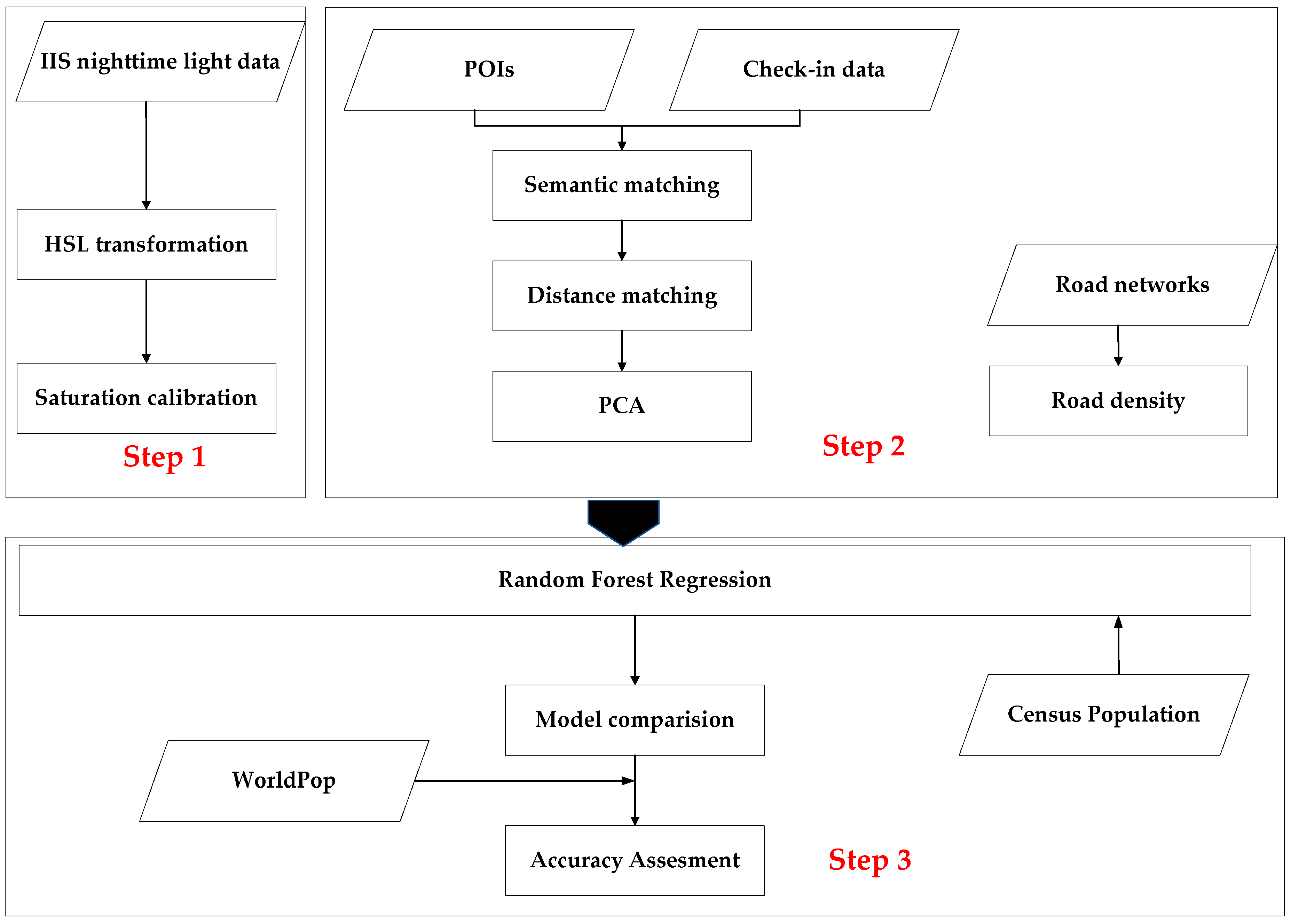
3.1. Flowcharts
3.2. Preprocessing of ISS Photography
3.3. Similarity Matching of Mobile Check-In Data and POI Data
3.3.1. Semantic Similarity Matching
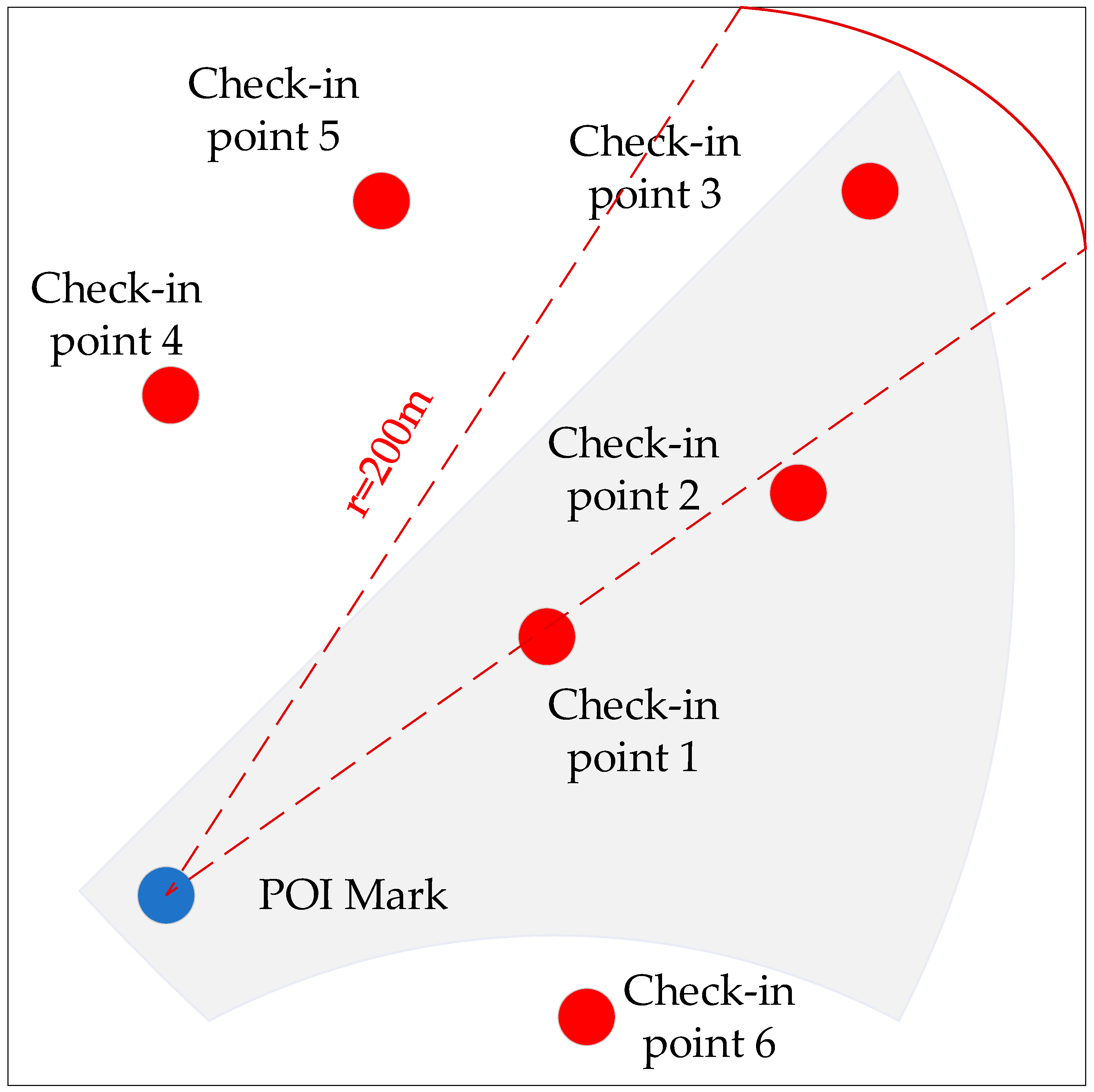
3.3.2. Distance Similarity Matching
3.4. Principal Component Analysis of Point of Intrests Data
3.5. Population Mapping with RF Model
4. Results
4.1. HSL and VANUI Calibration Results of ISS Photography
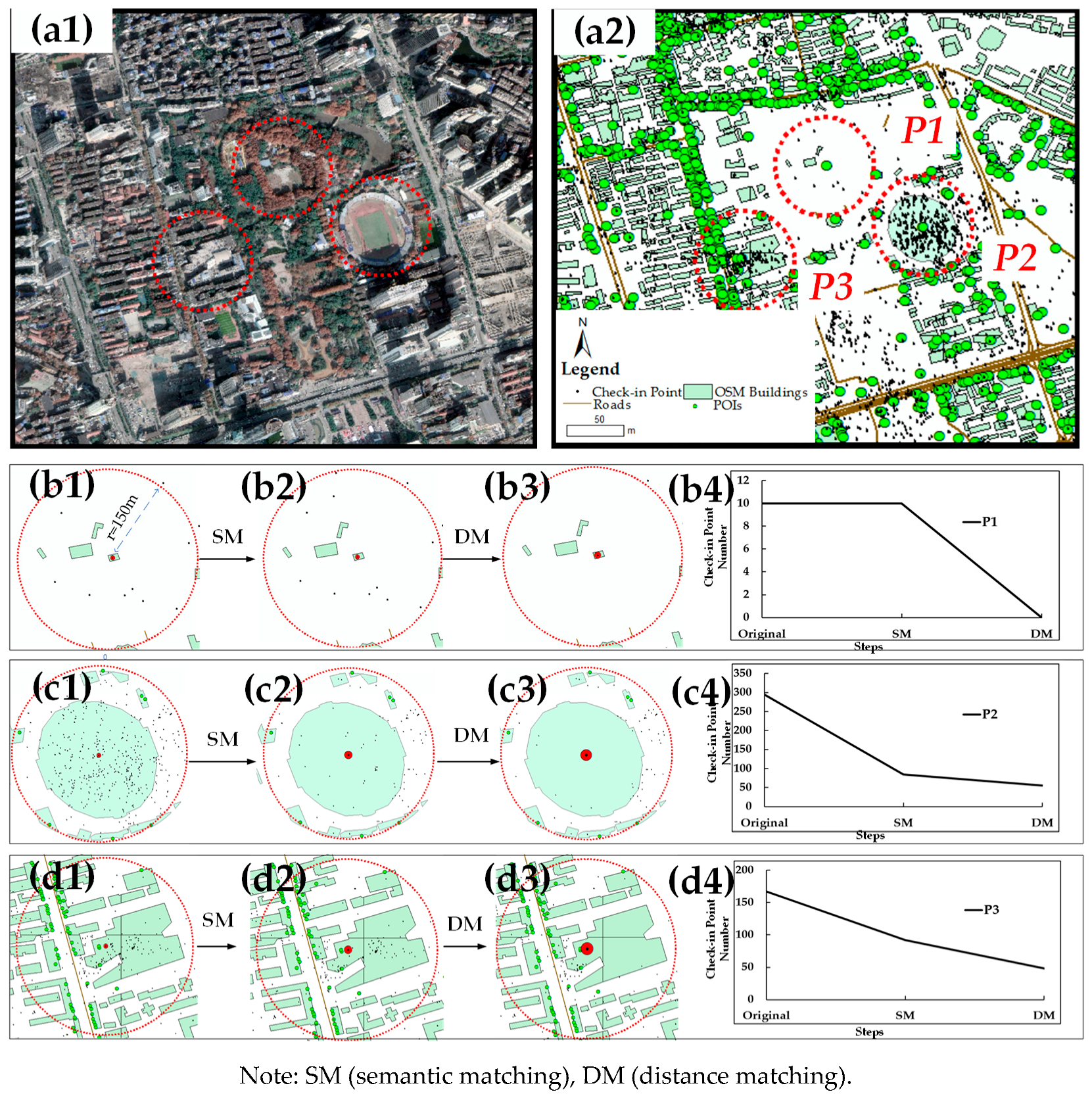
4.2. Results of Similarity Matching
4.3. Results of Principal Component Analysis
4.4. Results of Population Mapping
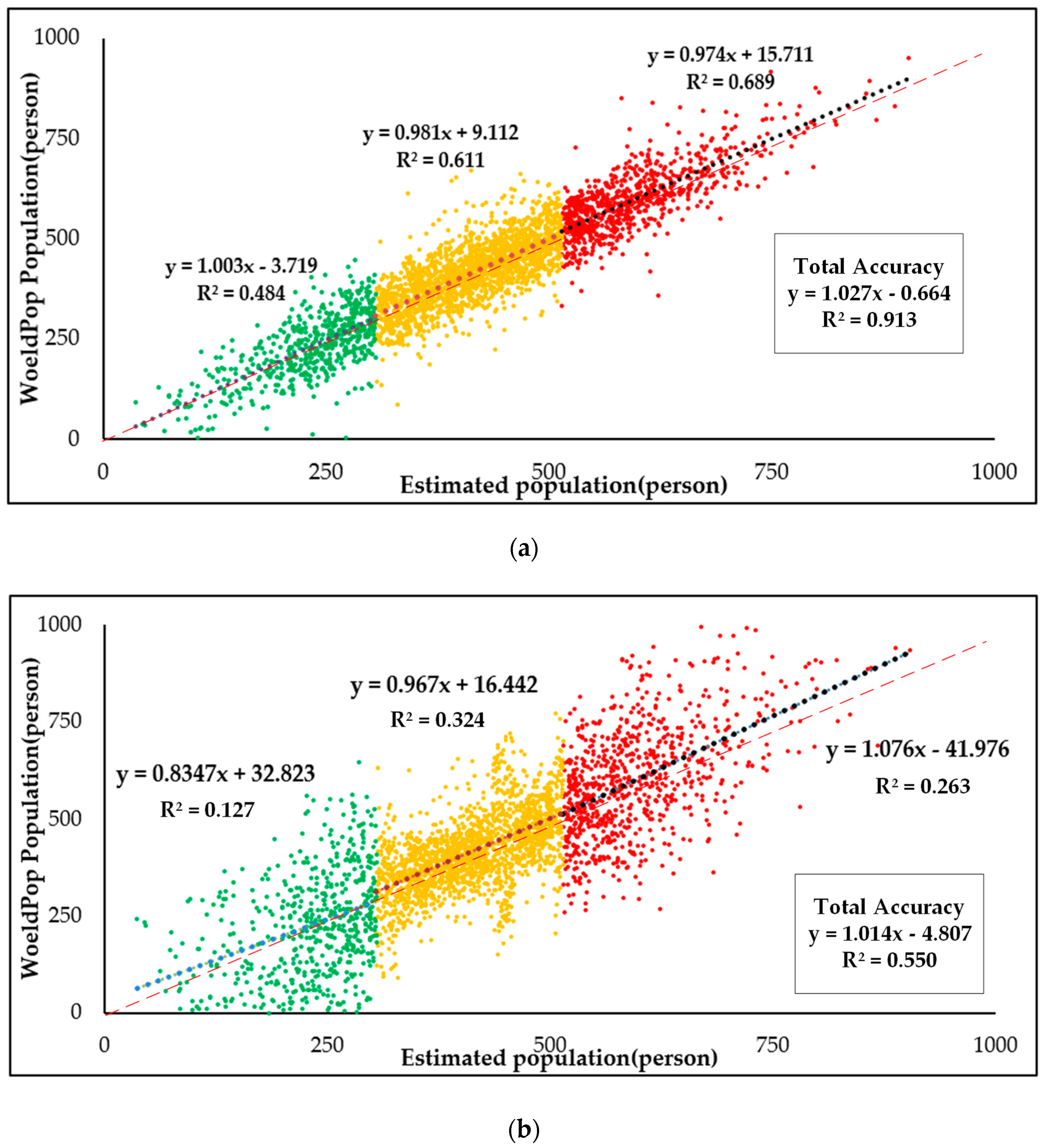
4.5. Accuracy Assesment
5. Discussion
5.1. Advantages of Using Check-In Data
5.2. Influence of Check-In Data Volume
5.3. Influence of the Acquisition Time of Check-In Data
6. Conclusions
Author Contributions
Funding
Acknowledgments
Conflicts of Interest
References
- Deville, P.; Linard, C.; Martin, S.; Gilbert, M.; Stevens, F.R.; Gaughan, A.E.; Blondel, V.D.; Tatem, A.J. Dynamic population mapping using mobile phone data. Proc. Natl. Acad. Sci. USA 2014, 111, 15888–15893. [Google Scholar] [CrossRef] [PubMed]
- Tatem, A.; Linard, C. Population mapping of poor countries. Nature 2011, 474, 36. [Google Scholar] [CrossRef] [PubMed]
- Ural, S.; Hussain, E.; Shan, J. Building population mapping with aerial imagery and GIS data. Int. J. Appl. Earth Obs. Geoinf. 2011, 13, 841–852. [Google Scholar] [CrossRef]
- Patel, N.N.; Stevens, F.R.; Huang, Z.; Gaughan, A.E.; Elyazar, I.; Tatem, A.J. Improving Large Area Population Mapping Using Geotweet Densities. Trans. GIS 2017, 21, 317–331. [Google Scholar] [CrossRef] [PubMed]
- Weber, E.M.; Seaman, V.Y.; Stewart, R.N.; Bird, T.J.; Tatem, A.J.; Mckee, J.J.; Bhaduri, B.L.; Moehl, J.J.; Reith, A.E. Census-independent population mapping in northern Nigeria. Remote Sens. Environ. 2018, 204, 786–798. [Google Scholar] [CrossRef]
- Zhou, Y. China’s Urbanization Levels: Reconstructing a Baseline from the Fifth Population Census. China Q. 2003, 173, 176–196. [Google Scholar]
- Office, P.N.G.N.S. 1980 National Population Census, Final Figures: National Summary; National Statistical Office: Port Moresby, Papua New Guinea, 1988. [Google Scholar]
- Hay, D.R. Cigarette smoking in New Zealand: Results from the 1976 population census. N. Z. Med. J. 1978, 111, 135–138. [Google Scholar]
- Hongqi, C.Z.M.; Chen, Z. Patterns of Inter-provincial Migration in China: Evidence from the Sixth Population Census. Popul. Res. 2012, 36, 87–99. [Google Scholar]
- Li, S.M. Population Migration and Urbanization in China: A Comparative Analysis of the 1990 Population Census and the 1995 National One Percent Sample Population Survey. Int. Migr. Rev. 2004, 38, 655–685. [Google Scholar] [CrossRef]
- Morton, T.A.; Yuan, F. Analysis of population dynamics using satellite remote sensing and US census data. Geocarto Int. 2009, 24, 143–163. [Google Scholar] [CrossRef]
- Amaral, S.; Gavlak, A.A.; Escada, M.I.S.; Monteiro, A.M.V. Using remote sensing and census tract data to improve representation of population spatial distribution: Case studies in the Brazilian Amazon. Popul. Environ. 2012, 34, 142–170. [Google Scholar] [CrossRef]
- Amaral, S.; Camara, G.; Monteiro, A.M.V.; Quintanilha, J.A.; Elvidge, C.D. Estimating population and energy consumption in Brazilian Amazonia using DMSP night-time satellite data. Comput. Environ. Urban Syst. 2005, 29, 179–195. [Google Scholar] [CrossRef]
- Cheng, L.; Yi, Z.; Wang, L.; Wang, S.; Cong, D. An estimate of the city population in China using DMSP night-time satellite imagery. In Proceedings of the IEEE International Geoscience & Remote Sensing Symposium, Barcelona, Spain, 23–28 July 2007. [Google Scholar]
- Linard, C.; Gilbert, M.; Snow, R.W.; Noor, A.M.; Tatem, A.J. Population Distribution, Settlement Patterns and Accessibility across Africa in 2010. PLoS ONE 2012, 7, e31743. [Google Scholar]
- Hillson, R.; Alejandre, J.D.; Jacobsen, K.H.; Ansumana, R.; Bockarie, A.S.; Bangura, U.; Lamin, J.M.; Malanoski, A.P.; Stenger, D.A. Methods for Determining the Uncertainty of Population Estimates Derived from Satellite Imagery and Limited Survey Data: A Case Study of Bo City, Sierra Leone. PLoS ONE 2014, 9, e11224. [Google Scholar]
- Mossoux, S.; Kervyn, M.; Soulé, H.; Canters, F. Mapping Population Distribution from High Resolution Remotely Sensed Imagery in a Data Poor Setting. Remote Sens. 2018, 10, 1409. [Google Scholar] [CrossRef]
- Li, X.; Guofan, S. Object-Based Land-Cover Mapping with High Resolution Aerial Photography at a County Scale in Midwestern USA. Remote Sens. 2014, 6, 11372–11390. [Google Scholar] [CrossRef]
- Han, D.; Yang, X.; Cai, H.; Xu, X.; Qiao, Z.; Cheng, C.; Dong, N.; Huang, D.; Liu, A. Modelling spatial distribution of fine-scale populations based on residential properties. Int. J. Remote Sens. 2019, 40, 5287–5300. [Google Scholar] [CrossRef]
- Shen, J.; Huang, Y. The working and living space of the ‘floating population’ in China. Asia Pac. Viewp. 2003, 44, 51–62. [Google Scholar] [CrossRef]
- Chen, X.; Yang, H.Z. The Research of Chinese Living Space Based on Phenomenology. Adv. Mater. Res. 2012, 598, 22–26. [Google Scholar] [CrossRef]
- Liu, Y.; Wang, Y.; Peng, J.; Du, Y.; Liu, X.; Li, S.; Zhang, D. Correlations between Urbanization and Vegetation Degradation across the World’s Metropolises Using DMSP/OLS Nighttime Light Data. Remote Sens. 2015, 7, 2067–2088. [Google Scholar] [CrossRef]
- Huang, Q.; Xi, Y.; Bin, G.; Yang, Y.; Zhao, Y. Application of DMSP/OLS Nighttime Light Images: A Meta-Analysis and a Systematic Literature Review. Remote Sens. 2014, 6, 6844–6866. [Google Scholar] [CrossRef]
- Guo, W.; Lu, D.; Wu, Y.; Zhang, J. Mapping Impervious Surface Distribution with Integration of SNNP VIIRS-DNB and MODIS NDVI Data. Remote Sens. 2015, 7, 12459–12477. [Google Scholar] [CrossRef]
- Yu, S.; Zhang, Z.; Liu, F. Monitoring population evolution in China using time-series DMSP/OLS nightlight imagery. Remote Sens. 2018, 10, 194. [Google Scholar] [CrossRef]
- Yang, X.; Ye, T.; Zhao, N.; Chen, Q.; Yue, W.; Qi, J.; Zeng, B.; Jia, P. Population Mapping with Multisensor Remote Sensing Images and Point-Of-Interest Data. Remote Sens. 2019, 11, 574. [Google Scholar] [CrossRef]
- Mohamadi, B.; Chen, S.; Liu, J. Evacuation Priority Method in Tsunami Hazard Based on DMSP/OLS Population Mapping in the Pearl River Estuary, China. ISPRS Int. J. Geo-Inf. 2019, 8, 137. [Google Scholar] [CrossRef]
- Zhuo, L.; Ichinose, T.; Zheng, J.; Chen, J.; Shi, P.J.; Li, X. Modelling the population density of China at the pixel level based on DMSP/OLS non-radiance-calibrated night-time light images. Int. J. Remote Sens. 2009, 30, 1003–1018. [Google Scholar] [CrossRef]
- Hao, R.; Yu, D.; Sun, Y.; Cao, Q.; Liu, Y.; Liu, Y.P. Integrating Multiple Source Data to Enhance Variation and Weaken the Blooming Effect of DMSP-OLS Light. Remote Sens. 2015, 7, 1422–1440. [Google Scholar] [CrossRef]
- Liu, Q.; Cao, C.; Weng, F. Striping in the Suomi NPP VIIRS Thermal Bands through Anisotropic Surface Reflection. J. Atmos. Ocean. Technol. 2013, 30, 2478–2487. [Google Scholar] [CrossRef]
- Wei, J.; He, G.; Liu, H. Modelling regional socio-economic parameters based on comparison of NPP / VIIRS and DMSP/OLS nighttime light imagery. Remote Sens. Inf. 2016, 4, 28–34. [Google Scholar]
- Li, X.; Li, D.; Xu, H.; Wu, C. Intercalibration between DMSP/OLS and VIIRS night-time light images to evaluate city light dynamics of Syria’s major human settlement during Syrian Civil War. Int. J. Remote Sens. 2017, 38, 1–18. [Google Scholar] [CrossRef]
- Shi, K.; Huang, C.; Yu, B.; Yin, B.; Huang, Y.; Wu, J. Evaluation of NPP-VIIRS night-time light composite data for extracting built-up urban areas. Remote Sens. Lett. 2014, 5, 358–366. [Google Scholar] [CrossRef]
- Hu, Y.; Zhao, G.; Zhang, Q.L. Spatial Distribution of Population Data Based on Nighttime Light and LUC Data in the SichuanChongqing Region. J. Geo-Inf. Sci. 2018, 20, 68–78. [Google Scholar]
- Huang, C.; Chen, Y.; Wu, J.; Li, L.; Liu, R. An evaluation of Suomi NPP-VIIRS data for surface water detection. Remote Sens. Lett. 2015, 6, 155–164. [Google Scholar] [CrossRef]
- Stokes, E.C.; Roman, M.O.; Seto, K.C. The Urban Social and Energy Use Data Embedded in Suomi-NPP VIIRS Nighttime Lights: Algorithm Overview and Status. In Proceedings of the Agu Fall Meeting, San Francisco, CA, USA, 15–19 December 2014. [Google Scholar]
- Amaral, S.; Monteiro, A.M.V.; Camara, G.; Quintanilha, J.A. DMSP/OLS night-time light imagery for urban population estimates in the Brazilian Amazon. Int. J. Remote Sens. 2006, 27, 855–870. [Google Scholar] [CrossRef]
- Bagan, H. Spatio-Temporal Dynamics of Urban Expansion in Japan Using Gridded Land Use Data, Population Census Data and DMSP Data. Proceedings of Agu Fall Meeting, San Francisco, CA, USA, 15–19 December 2014. [Google Scholar]
- Tan, M.; Li, X.; Li, S.; Xin, L.; Wang, X.; Li, Q.; Li, W.; Li, Y.; Xiang, W. Modeling population density based on nighttime light images and land use data in China. Appl. Geogr. 2018, 90, 239–247. [Google Scholar] [CrossRef]
- Briggs, D.J.; Gulliver, J.; Fecht, D.; Vienneau, D.M. Dasymetric modelling of small-area population distribution using land cover and light emissions data. Remote Sens. Environ. 2007, 108, 451–466. [Google Scholar] [CrossRef]
- Lu, D.; Tian, H.; Zhou, G.; Ge, H. Regional mapping of human settlements in southeastern China with multisensor remotely sensed data. Remote Sens. Environ. 2015, 112, 3668–3679. [Google Scholar] [CrossRef]
- Ma, T. Multi-Level Relationships between Satellite-Derived Nighttime Lighting Signals and Social Media–Derived Human Population Dynamics. Remote Sens. 2018, 10, 1128. [Google Scholar] [CrossRef]
- Huang, H.; Li, Q.; Zhang, Y. Urban Residential Land Suitability Analysis Combining Remote Sensing and Social Sensing Data: A Case Study in Beijing, China. Sustainability 2019, 11, 2255. [Google Scholar] [CrossRef]
- Stevens, F.R.; Gaughan, A.E.; Linard, C.; Tatem, A.J. Disaggregating Census Data for Population Mapping Using Random Forests with Remotely-Sensed and Ancillary Data. PLoS ONE 2014, 10, e0107042. [Google Scholar] [CrossRef]
- Ye, T.; Zhao, N.; Yang, X.; Ouyang, Z.; Liu, X.; Chen, Q.; Hu, K.; Yue, W.; Qi, J.; Li, Z.; et al. Improved population mapping for China using remotely sensed and points-of-interest data within a random forests model. Sci. Total Environ. 2019, 658, 936–946. [Google Scholar] [CrossRef] [PubMed]
- Malleson, N.; Andresen, M.A. The impact of using social media data in crime rate calculations: Shifting hot spots and changing spatial patterns. Cartogr. Geogr. Inf. Sci. 2015, 42, 112–121. [Google Scholar] [CrossRef]
- Castillo, C. Validity: Biases and Pitfalls of Social Media Data. Big Crisis Data: Social Media in Disasters and Time-Critical Situations; Cambridge University Press: Cambridge, UK, 2016; pp. 123–137. [Google Scholar]
- Gu, Y.; Qian, Z.; Chen, F. From Twitter to detector: Real-time traffic incident detection using social media data. Transp. Res. Part C 2016, 67, 321–342. [Google Scholar] [CrossRef]
- Liu, Y.; Sui, Z.; Kang, C. Uncovering Patterns of Inter-Urban Trip and Spatial Interaction from Social Media Check-In Data. PLoS ONE 2014, 9, e86026. [Google Scholar] [CrossRef] [PubMed]
- Ying, J.C.; Lu, H.C.; Kuo, W.N.; Tseng, V.S. Urban point-of-interest recommendation by mining user check-in behaviors. In Proceedings of the Acm Sigkdd International Workshop on Urban Computing, Beijing, China, 12–12 August 2012. [Google Scholar]
- Kotarba, A.Z.; Aleksandrowicz, S. Impervious surface detection with nighttime photography from the International Space Station. Remote Sens. Environ. 2016, 176, 295–307. [Google Scholar] [CrossRef]
- Dawson, M.; Evans, C.; Stefanov, W.; Wilkinson, M.J.; Willis, K.; Runco, S. Human Settlements in the South-Central U.S., Viewed at Night from the International Space Station. In Proceedings of the International Conference on Pipelines & Trenchless Technology, Wuhan, China, 19–22 October 2012. [Google Scholar]
- Li, Q.; Lu, L.; Weng, Q.; Xie, Y.; Guo, H. Monitoring Urban Dynamics in the Southeast U.S.A. Using Time-Series DMSP/OLS Nightlight Imagery. Remote Sens. 2016, 8, 578. [Google Scholar] [CrossRef]
- Liu, X.; Hu, G.; Ai, B.; Li, X.; Shi, Q. A Normalized Urban Areas Composite Index (NUACI) Based on Combination of DMSP-OLS and MODIS for Mapping Impervious Surface Area. Remote Sens. 2015, 7, 17168–17189. [Google Scholar] [CrossRef]
- Liang, Z.; Bao, M.; Yang, N.; Lao, Y.; Yun, Z.; Tian, Y. Spatio-temporal Analysis of Weibo Check-in Data Based on Spatial Data Warehouse. Commun. Comput. Inf. Sci. 2013, 399, 466–479. [Google Scholar]
- VanVoorhis, B.A.; Dark, V.J. Semantic matching, response mode, and response mapping as contributors to retroactive and proactive priming. J. Exp. Psychol. Learn. Mem. Cogn. 1995, 21, 913–932. [Google Scholar] [CrossRef]
- Bordes, A.; Glorot, X.; Weston, J.; Bengio, Y. A semantic matching energy function for learning with multi-relational data. Mach. Learn. 2014, 94, 233–259. [Google Scholar] [CrossRef]
- Shamdasani, J.; Bloodsworth, P.; Munir, K.; Rahmouni, H.B.; Mcclatchey, R. MedMatch—Towards Domain Specific Semantic Matching. Lect. Notes Comput. Sci. 2011, 6828, 375–382. [Google Scholar]
- Giunchiglia, F.; Yatskevich, M.; Giunchiglia, E. Efficient Semantic Matching. In Proceedings of the European Conference on the Semantic Web: Research & Applications, Heraklion, Greece, 10–12 May 2004. [Google Scholar]
- Sánchez-Martínez, F.; Martínez-Sempere, I.; Ivars-Ribes, X.; Carrasco, R.C. An open diachronic corpus of historical Spanish: Annotation criteria and automatic modernisation of spelling. Comput. Sci. 2013, 47, 1327–1342. [Google Scholar]
- Tobler, W.R. Supplement: Proceedings. International Geographical Union. Commission on Quantitative Methods—A Computer Movie Simulating Urban Growth in the Detroit Region. Econ. Geogr. 1970, 46, 234–240. [Google Scholar] [CrossRef]
- Kwon, O.K.; Kim, D.; Suh, J.W. Accurate M-hausdorff distance similarity combining distance orientation for matching multi-modal sensor images. Pattern Recognit. Lett. 2011, 32, 903–909. [Google Scholar] [CrossRef]
- Xu, H.-Y.; Fang, X.; Feng, Y. Improvement of semantic distance-based concept similarity computation in Web service matching. J. Comput. Appl. 2011, 31, 2808–2810. [Google Scholar]
- Wang, L.; Fan, H.; Wang, Y. Site Selection of Retail Shops Based on Spatial Accessibility and Hybrid BP Neural Network. ISPRS Int. J. Geo-Inf. 2018, 7, 202. [Google Scholar] [CrossRef]
- Song, H.; Chen, G.; Yang, W. Principal component analysis for hyper spectral image classification. Eng. Surv. Mapp. 2017, 62, 115–122. [Google Scholar]
- Perdiguero-Alonso, D.; Montero, F.E.; Kostadinova, A.; Raga, J.A.; Barrett, J. Random forests, a novel approach for discrimination of fish populations using parasites as biological tags. Int. J. Parasitol. 2008, 38, 1425–1434. [Google Scholar] [CrossRef]
- Stephan, J.; Stegle, O.; Beyer, A. A random forest approach to capture genetic effects in the presence of population structure. Nat. Commun. 2015, 6, 7432. [Google Scholar] [CrossRef]
- Mascaro, J.; Asner, G.P.; Knapp, D.E.; Kennedybowdoin, T.; Martin, R.E.; Anderson, C.; Higgins, M.; Chadwick, K.D. A tale of two “forests”: Random forest machine learning AIDS tropical forest carbon mapping. PLoS ONE 2014, 9, e85993. [Google Scholar] [CrossRef]
- Maxwell, A.E.; Warner, T.A.; Strager, M.P. Predicting Palustrine Wetland Probability Using Random Forest Machine Learning and Digital Elevation Data-Derived Terrain Variables. Photogramm. Eng. Remote Sens. 2016, 82, 437–447. [Google Scholar] [CrossRef]
- Belgiu, M.; Drăguţ, L. Random forest in remote sensing: A review of applications and future directions. ISPRS J. Photogramm. Remote Sens. 2016, 114, 24–31. [Google Scholar] [CrossRef]
- Li, K.; Chen, Y.; Li, Y. The Random Forest-Based Method of Fine-Resolution Population Spatialization by Using the International Space Station Nighttime Photography and Social Sensing Data. Remote Sens. 2018, 10, 1650. [Google Scholar] [CrossRef]
- Wang, L.; Fan, H.; Wang, Y. Sustainability Analysis and Market Demand Estimation in the Retail Industry through a Convolutional Neural Network. Sustainability 2018, 10, 1762. [Google Scholar] [CrossRef]
- Lebel, L.; Garden, P.; Banaticla, M.R.N.; Lasco, R.D.; Contreras, A.; Mitra, A.P.; Sharma, C.; Nguyen, H.T.; Ooi, G.L.; Sari, A. Management into the Development Strategies of Urbanizing Regions in Asia: Implications of Urban Function, Form, and Role . J. Ind. Ecol. 2010, 11, 61–81. [Google Scholar]
- Shen, Y.; Karimi, K. Urban function connectivity: Characterisation of functional urban streets with social media check-in data. Cities 2016, 55, 9–21. [Google Scholar] [CrossRef]
- Li, M.; Shen, Z.; Hao, X. Revealing the relationship between spatio-temporal distribution of population and urban function with social media data. GeoJournal 2016, 81, 919–935. [Google Scholar] [CrossRef]
- Hsieh, H.P.; Li, C.T.; Lin, S.D. Exploiting large-scale check-in data to recommend time-sensitive routes. In Proceedings of the ACM SIGKDD International Workshop on Urban Computing, Beijing, China, 12 August 2012. [Google Scholar]
- Hsieh, H.P.; Li, C.T. Mining Time-Aware Transit Patterns for Route Recommendation in Big Check-in Data. In Proceedings of the Pacific-asia Conference on Knowledge Discovery & Data Mining, Tainan, Taiwan, 13–16 May 2014. [Google Scholar]
- Guo, X.; Shao, Q.; Li, Y.; Wang, Y.; Wang, D.; Liu, J.; Fan, J.; Yang, F. Application of UAV Remote Sensing for a Population Census of Large Wild Herbivores—Taking the Headwater Region of the Yellow River as an Example. Remote Sens. 2018, 10, 1041. [Google Scholar] [CrossRef]


| Matched Check-In Points | POIs | Rate (%) | Top 3 Maximum POI Categories | Average |
|---|---|---|---|---|
| ≥20 | 7486 | 3.901 | Shopping malls, residential quarters, catering facilities | 33 |
| ≥10 and <20 | 69,532 | 36.261 | Shopping malls, residential quarters, attractions | 15 |
| ≥1 and <10 | 103,425 | 53.926 | Catering facilities, government agencies, hotel facilities | 6 |
| 0 | 11,342 | 5.912 | Auto service facilities, cultural facilities, factories | 0 |
| Category | POI Number | Number of Check-In Points | Average Check-In Points | Maximum Number of Check-In Points |
|---|---|---|---|---|
| Catering facilities | 43,909 | 491,294 | 11.19 | 242 |
| Auto service facilities | 539 | 172 | 0.32 | 14 |
| Sports facilities | 3459 | 6185 | 1.79 | 21 |
| Residential quarters | 41,041 | 493,514 | 12.02 | 395 |
| Shopping malls | 43,093 | 480,311.9254 | 11.15 | 199 |
| Life service facilities | 8304 | 67,162 | 8.09 | 87 |
| Medical facilities | 3872 | 40,720 | 10.52 | 174 |
| Hotel facilities | 3551 | 83,578 | 23.54 | 89 |
| Attractions | 4825 | 87,523 | 18.14 | 105 |
| Government agencies | 9725 | 113,436 | 11.66 | 95 |
| Cultural facilities | 4486 | 0.00 | 74 | |
| Traffic stations | 8474 | 29,683 | 3.50 | 23 |
| Financial facilities | 1626 | 1592 | 0.98 | 12 |
| Landmarks | 2875 | 3803 | 1.32 | 25 |
| Factories | 2421 | 2418 | 1.00 | 14 |
| Communal facilities | 8975 | 10,789 | 1.20 | 31 |
| Sum | 191,175 | 1,912,181 | 10.00 |
| Component | Variance (%) | Cumulative (%) | Component | Variance (%) | Cumulative (%) |
|---|---|---|---|---|---|
| 1 | 34.275 | 30.275 | 9 | 1.032 | 98.143 |
| 2 | 23.212 | 57.487 | 10 | 0.712 | 98.855 |
| 3 | 17.711 | 75.198 | 11 | 0.57 | 99.425 |
| 4 | 10.658 | 85.856 | 12 | 0.207 | 99.632 |
| 5 | 4.226 | 90.082 | 13 | 0.175 | 99.807 |
| 6 | 3.029 | 93.111 | 14 | 0.126 | 99.933 |
| 7 | 2.075 | 95.186 | 15 | 0.058 | 99.991 |
| 8 | 1.925 | 97.111 | 16 | 0.009 | 100 |
| Variable | Component 1 | Component 2 | Component 3 | Component 4 |
|---|---|---|---|---|
| Catering facilities | 0.558 | 0.081 | 0.074 | −0.101 |
| Auto service facilities | 0.002 | −0.177 | 0.156 | 0.004 |
| Sports facilities | 0.082 | 0.101 | −0.112 | 0.063 |
| Residential quarters | 0.126 | 0.492 | 0.073 | −0.172 |
| Shopping malls | 0.494 | 0.079 | −0.276 | 0.024 |
| Life service facilities | 0.429 | 0.319 | 0.047 | −0.024 |
| Medical facilities | 0.137 | 0.142 | 0.291 | 0.095 |
| Hotel facilities | −0.062 | 0.004 | 0.067 | 0.249 |
| Communal facilities | 0.042 | −0.248 | 0.295 | 0.044 |
| Attractions | 0.036 | −0.164 | 0.135 | 0.029 |
| Government agencies | −0.294 | 0.041 | 0.094 | 0.117 |
| Cultural facilities | 0.056 | 0.108 | 0.071 | 0.071 |
| Traffic stations | 0.204 | 0.095 | −0.097 | 0.103 |
| Financial facilities | 0.075 | 0.008 | 0.108 | 0.096 |
| Landmarks | −0.206 | −0.285 | 0.134 | 0.059 |
| Factories | 0.007 | −0.102 | 0.085 | −0.198 |
© 2019 by the authors. Licensee MDPI, Basel, Switzerland. This article is an open access article distributed under the terms and conditions of the Creative Commons Attribution (CC BY) license (http://creativecommons.org/licenses/by/4.0/).
Share and Cite
Wang, L.; Fan, H.; Wang, Y. Fine-Resolution Population Mapping from International Space Station Nighttime Photography and Multisource Social Sensing Data Based on Similarity Matching. Remote Sens. 2019, 11, 1900. https://doi.org/10.3390/rs11161900
Wang L, Fan H, Wang Y. Fine-Resolution Population Mapping from International Space Station Nighttime Photography and Multisource Social Sensing Data Based on Similarity Matching. Remote Sensing. 2019; 11(16):1900. https://doi.org/10.3390/rs11161900
Chicago/Turabian StyleWang, Luyao, Hong Fan, and Yankun Wang. 2019. "Fine-Resolution Population Mapping from International Space Station Nighttime Photography and Multisource Social Sensing Data Based on Similarity Matching" Remote Sensing 11, no. 16: 1900. https://doi.org/10.3390/rs11161900
APA StyleWang, L., Fan, H., & Wang, Y. (2019). Fine-Resolution Population Mapping from International Space Station Nighttime Photography and Multisource Social Sensing Data Based on Similarity Matching. Remote Sensing, 11(16), 1900. https://doi.org/10.3390/rs11161900