Multipath Residual Network for Spectral-Spatial Hyperspectral Image Classification

Abstract

Convolutional neural networks (CNNs) have recently shown outstanding capability for hyperspectral image (HSI) classification. In this work, a novel CNN model is proposed, which is wider than other existing deep learning-based HSI classification models. Based on the fact that very deep residual networks (ResNets) behave like ensembles of relatively shallow networks, our proposed network, called multipath ResNet (MPRN), employs multiple residual functions in the residual blocks to make the network wider, rather than deeper. The proposed network consists of shorter-medium paths for efficient gradient flow and replaces the stacking of multiple residual blocks in ResNet with fewer residual blocks but more parallel residual functions in each of it. Experimental results on three real hyperspectral data sets demonstrate the superiority of the proposed method over several state-of-the-art classification methods.

1. Introduction

Remote sensing hyperspectral images (HSIs) usually contain information about hundreds of spectral bands spanning from visible to infrared spectrum. Each pixel in HSIs is a high-dimensional vector whose entries correspond to the spectral reflectance in a specific wavelength, providing rich spectral information for distinguishing land covers of interest [1]. Recently, HSI classification with the aim of identifying the land-cover type of each pixel has become one of the most active research fields in the remote sensing community, because it is an essential step in a wide variety of earth monitoring applications, such as environmental monitoring [2] and precision agriculture [3].

The spectral and the spatial information of HSIs are two major characteristics that can be exploited for classification [4]. Traditional classification methods such as random forest [5], support vector machine (SVM) [6] and multinomial logistic regression [7], mainly focus on making use of the abundant spectral information for classification. To improve classification performance, methods such as morphological profiles [8], multiple kernel learning [9], superpixel [10] and sparse representation [11] have been introduced to combine the spatial information with the spectral information for HSI classification [12,13]. For instance, Benediktsson et al. utilized extended morphological profiles (EMPs) to obtain spectral-spatial features of HSIs [8]. Fang et al. proposed a multiscale adaptive sparse representation (MASR) model to exploit the multiscale spatial information of HSIs [11]. Fauvel et al. proposed a morphological kernel based SVM classifier to jointly use the spatial and the spectral information for classification [14]. Nevertheless, the common limitation of these methods is that they heavily rely on hand-crafted features, which require experts’ experiences and massive efforts in feature engineering, limiting their applicability in difficult scenarios.

Recently, deep learning-based methods have made great breakthroughs in many computer vision tasks, for example, image classification [15,16], semantic segmentation [17], natural language processing [18] and object detection [19], for they can automatically extract robust and discriminative features from original data in a hierarchical way. Deep learning models have also been introduced for HSI classification and have achieved a remarkable progress [20,21]. In Reference [22], a stacked auto-encoder (SAE) was first proposed for HSI spectral classification. Next, deep learning models, including deep belief network (DBN) [23] and convolutional neural network (CNN) [24,25,26], were introduced as deep spectral classifiers for HSI classification. To make use of both the spectral and spatial information of HSIs, a series of improved CNN-based spectral–spatial classifiers were then proposed [27,28,29]. Zhao et al. proposed a spectral-spatial feature-based classification (SSFC) framework in which the CNN was used to extract spatial features and the balanced local discriminant embedding method to extract spectral features [30]. To simultaneously extract the spectral-spatial features of HSIs, 3-D CNNs were proposed for HSI classification [31,32]. Due to the joint utilization of the spectral and spatial information of HSIs, spectral-spatial classifiers usually achieve better classification performance than spectral classifiers. To extract deeper discriminative spectral-spatial features, residual learning [33], which helps to train CNNs up to thousands of layers without suffering gradient vanishing, was introduced for HSI classification [34,35,36,37,38,39]. For instance, a fully convolutional neural network was proposed for HSI classification in which multiscale filter bank was used to exploit both spectral and spatial information embedded in HSIs and residual learning to enhance the learning efficiency of the network [34]. Song et al. proposed a deep feature fusion network in which multiple-layer features extracted from a deep CNN were fused for classification and residual learning was utilized to alleviate gradient vanishing problem [35].

Although residual learning helps to extremely increase the network depth, recent studies pointed out that deep ResNets actually behave like a large ensemble of much shallower networks, instead of a ultra deep network [40,41]. By rewriting ResNets as an explicit collection of paths of different length, Veit et al. revealed that although these paths are trained together, they exhibit ensemble-like behavior, that is, different paths are not strongly dependent on each other [40]. For example, the removal of a layer during the testing phase has a modest impact on the performance of a ResNet. Furthermore, deep paths do not contribute any gradient during training. For instance, most of the gradient in a 110-layer ResNet comes from paths between 10 to 34 layers deep, demonstrating that the effective paths are relatively shallow. Furthermore, a ResNet trained only on some effective paths can achieve a comparable performance to that of a full ResNet [40].

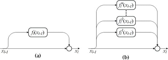
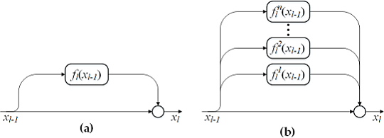
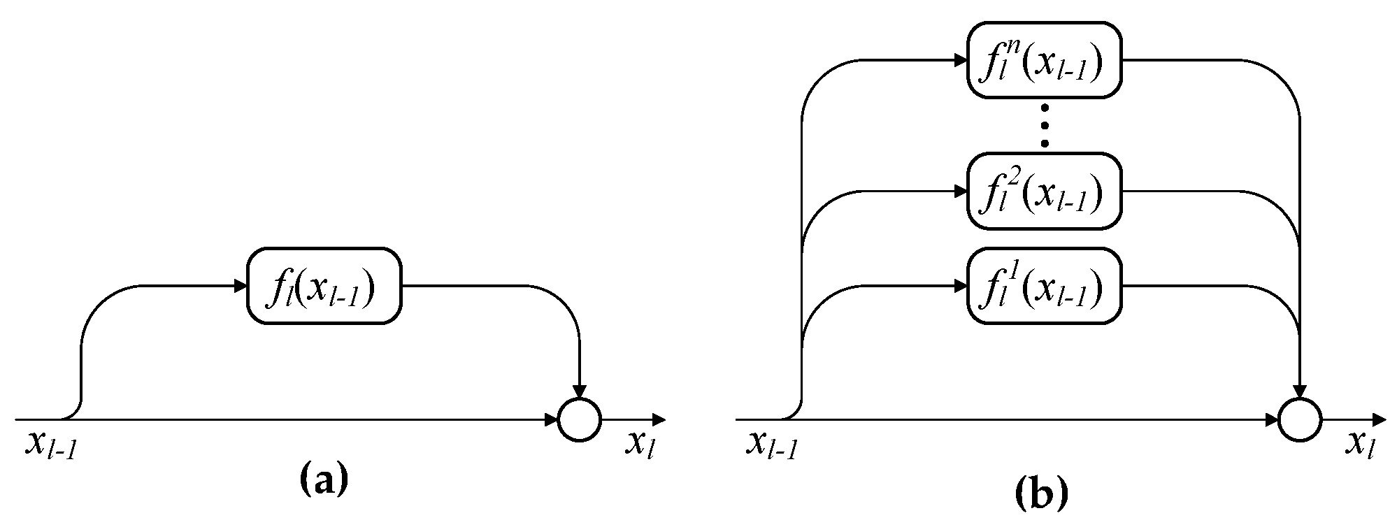
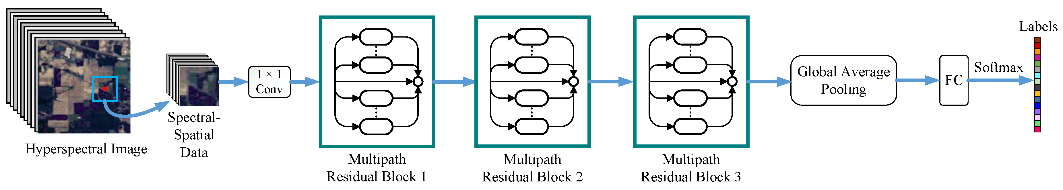
In this paper, inspired by the above observations, a novel multipath ResNet (MPRN) model that employs multiple residual functions in each residual block is proposed for HSI classification, utilizing both spectral and spatial information. Different from the previous networks used in HSI classification, the proposed network is wider and consists of shorter-medium paths for efficient gradient flow. The proposed network is more efficient than conventional ResNet, since deep paths, which do not contribute any gradient during training, are abandoned. The main contributions of this paper can be summarized as follows: (1) The increase of the number of residual functions in each residual block can enhance the performance of ResNet and can lead to a better performance than the increase of the network depth; (2) To the best of our knowledge, the idea of balancing network width and depth for accurate and efficient HSI classification is proposed for the first time in this paper; and (3) Experimental results on three real hyperspectral data sets demonstrate that the proposed method can achieve a better classification performance than several state-of-the-art approaches.

The remainder of this paper is organized as follows. Section 2 introduces the general framework of CNN-based HSI classification and reviews the ResNet briefly. In Section 3, the details of the proposed method are described. Experimental results conducted on three real hyperspectral data sets are then presented and discussed in Section 4. Finally, some conclusions and suggestions are provided in Section 5.

2. Related Work

2.1. CNN-Based HSI Classification

Let $U\in {\mathbb{R}}^{H\times W\times C}$ be an HSI data set, where H and W represent the height and the width of the spatial dimensions, respectively and C is the number of spectral bands. Instead of directly classifying each hyperspectral pixel vector, in CNN-based models an image patch centered at each pixel is generally taken for classification. In this way, the spatial and spectral information contained in such patches are combined in the task of classifying pixels, resulting in a reduction of the label uncertainty and intraclass variability [42].

Convolutional (Conv) layers are the key parts of a CNN model in which the input HSI patches or feature maps are convolved with convolution filter banks (also called convolution kernels) to produce feature maps as follows:

$$X_l=X_{l-1}\ast W_l+B_l,$$

(1)

where $X_{l-1}$ and $X_l$ represent the input and output of the lth Conv layer, respectively, $W_l$ and $B_l$ refer to the weights and biases of the Conv layer, respectively and ∗ stands for convolution operator.

To alleviate the gradient vanishing problem and speed up the training process in a deep CNN, a batch normalization (BN) layer [43] is placed behind each Conv layer to reduce the internal covariance shift by imposing a Gaussian distribution on each batch of feature maps, allowing a more independent learning process in each layer. The BN layer can be expressed as

$$BN\left(X_l\right)=\frac{X_l-mean\left[X_l\right]}{\sqrt{Var\left[X_l\right]+ϵ}}·\gamma +\beta ,$$

(2)

where $\gamma$ and $\beta$ are learnable parameter vectors, respectively and $ϵ$ is a parameter for numerical stability.

Following the BN layer, an activation layer is added to improve the nonlinearity of the network. To effectively avoid the vanishing gradient problem, a rectified linear unit (ReLU) is used as a nonlinear activation function [15]. In addition, a pooling layer is periodically placed behind several Conv layers in the CNN to reduce the size of feature maps, decreasing the amount of computation of the network. Then, fully connected (FC) layers are adopted to transform the size-reduced feature maps into a one-dimensional vector z, which is input to a softmax function to compute the class probability distribution for each pixel

$$p_i=\frac{e^{z_i}}{{\sum }_{j=1}^n{e}^{z_j}},i=1,2,\dots ,n,$$

(3)

where n refers to the number of classes. Finally, the predicted category of each pixel is determined by the maximal probability

$$class=\underset{i=1,2,\dots ,n}{argmax}{p}_i.$$

(4)

2.2. ResNet

It is well known that deeper networks usually lead to a better performance over shallower ones. However, training very deep networks is difficult due to the vanishing gradient problem, that is, gradient signals fade slightly when passing through each layer during the backpropagation process and become close to zero in shallower layers, hampering the convergence of the network from the beginning [44]. In addition, based on approximation theory, the hypothesis space “drifts” away from the true solution when adding more layers [45]. As a consequence, when extremely increasing network depth, the classification accuracy first saturates and then degrades rapidly. Deep ResNets avoid this problem by employing identity skip-connections, which help the gradient flowing back to the shallow layers without vanishing and facilitate the training of very deep networks up to thousands of layers [33].

ResNet is constructed by stacking multiple fundamental structural elements called residual blocks. Figure 1 illustrates the architecture of a typical residual block, called bottleneck residual block [46]. The residual block performs the following computation:

$$x_l=f_l\left(x_{l-1}\right)+x_{l-1},$$

(5)

where $x_{l-1}$ and $x_l$ are the input and output of the lth residual block, respectively and $f_l(·)$ denotes the residual function to be learned. As can be seen from the Figure 1, $f_l(·)$ consists of 3 convolutional (Conv) layers each of which is preceded by a batch normalization (BN) layer [43] and a ReLU activation function, which is known as the pre-activation [46]. The kernel size of three Conv layers are $1\times 1$, $3\times 3$ and $1\times 1$, respectively. Here the first $1\times 1$ layer is used to reduce feature dimension and the second $1\times 1$ layer to expand it back.

3. Methodology

This section is structured as follows. First, the phenomenon that deep ResNet behaves like a large ensemble of relatively shallow networks is described. Then, the proposed MPRN model is introduced. Finally, the HSI classification framework based on MPRN is described.

3.1. Deep ResNets Behave Like Ensembles

To better understand ResNets, Veit et al. interpreted them in an unraveled view and conducted a detailed experimental study revealing that ResNets act like ensembles of relatively shallow networks [40]. Consider a ResNet consisting of 3 residual blocks from input $x_0$ to output $x_3$. Its conventional graphical representation is shown in Figure 2a. Based on Equation (5), the computation process can be expressed as

$$\begin{array}{cc}\hfill x_3& =f_3\left(x_2\right)+x_2\hfill \\ & =f_3(f_2\left(x_1\right)+x_1)+[f_2\left(x_1\right)+x_1]\hfill \\ & =f_3(f_2(f_1\left(x_0\right)+x_0)+f_1\left(x_0\right)+x_0)+[f_2(f_1\left(x_0\right)+x_0)+f_1\left(x_0\right)+x_0].\hfill \end{array}$$

(6)

The graphical view of Equation (6) is illustrated in Figure 2b. It can be clearly seen that there are many paths that can be chosen when data flowing from the input to the output. Each path denotes a unique configuration that decides which residual function to perform and which to skip. For a ResNet consisting of m residual blocks, there will be $2^m$ number of possible paths from the input to the output (also known as the multiplicity of the network), which is different from classical networks such as AlexNet [15] or VGGNet [47], where input flows along a single path from input to output. Moreover, in classical networks, each layer depends only on the output of its previous layer. As for ResNets, each residual function $f_l(·)$ receives data with $2^{l-1}$ different distributions generated from every possible path of the previous $l-1$ residual blocks.

Note that paths in a ResNet are of differing length and the distribution of all possible path lengths follows a Binomial distribution. For instance, there is one path that passes through all residual functions and are m paths that only pass through one residual function. During training, shallow paths contribute more gradient than deep paths [40]. For example, for a 110-layer ResNet, only paths between 10 and 34 layers depth have significant contributions towards the gradient updates. These paths are called effective paths, which are relatively shallow compared with the network depth. Additionally, paths in a ResNet exhibit ensemble-like behavior, that is, they are not strongly depend on each other. In addition, the performance of a ResNet smoothly correlates with the number of effective paths. Moreover, deep paths are indeed not needed as they do not contribute any gradient during training, for example, a ResNet trained only on the effective paths can obtain comparable performance with a full ResNet [40].

3.2. MPRN

In previous methods, usually the depth of ResNets is increased for extracting deeper discriminative features to improve the classification performance [33,46]. However, every percentage of improvement demands significantly increase of the number of layers, for example, a 164-layer ResNet was with a test error rate of 5.46% and a 1001-layer ResNet of 4.92% on the CIFAR-10 image classification data set, whereas the latter model has six times more computational complexity than the former [33]. One possible reason for this problem is that the increase of depth cannot improve the network performance in an efficient manner, since deep paths do not contribute any gradient during training. In addition, wide ResNets that have 50 times few layers can outperform the original ResNet, indicating that the power of ResNet arises from the identity skip-connections rather than the extreme increase of the network depth [48].

To further improve the classification performance, in this work, a multipath ResNet (MPRN) is proposed in which each residual block consists of multiple residual functions, as shown in Figure 3b. By introducing multiple residual functions to Equation (5), the output of the lth block in MPRN can be computed as:

$$x_l=f_l^1\left(x_{l-1}\right)+f_l^2\left(x_{l-1}\right)+\cdots +f_l^n\left(x_{l-1}\right)+x_{l-1},$$

(7)

where $f_l^n(·)$ denotes the nth residual function in the lth residual block. In MPRN, all the residual functions have the same architecture as the residual function in the bottleneck residual block. Consider a MPRN with 3 residual blocks each of which has 2 residual functions. For the lth block, there are 4 possible paths for gradient flow: (1) performing $f_l^1$ and skipping $f_l^2$; (2) performing $f_l^2$ and skipping $f_l^1$; (3) performing both $f_l^1$ and $f_l^2$; and (4) skipping both $f_l^1$ and $f_l^2$. Therefore, the multiplicity of each block is 4 and the multiplicity of the whole network is $4^3$. Giving a MPRN with m residual blocks and n residual functions in each block, the multiplicity of each block is $2^n$ since every residual function can be either performed or skipped and the total multiplicity of MPRN is $2^{mn}$.

Now consider a baseline ResNet with m residual blocks and let c be a constant integer. To improve its classification performance, a deeper network can be constructed by increasing the number of residual blocks to $cm$. In addition, a wider network, that is, MPRN, can be constructed by increasing the number of residual functions in each block to c while keeping the number of residual blocks to m. Note that the two improved networks have the same number of residual functions, that is, $cm$ and thus the same number of parameters. In addition, the multiplicity of both networks are $2^{cm}$. However, compared with the deeper ResNet, MPRN has more shorter-medium paths that can significantly contribute gradient during training. This way not only enhances the efficiency of parameters utilization but also improves performance.

Let $[a,b]$ be the range of effective paths’ length (also known as the effective range) of the baseline ResNet. Due to the exponential reduction in the gradient magnitude during back propagation, the deeper ResNet is shifted and/or scaled toward a shallower network [40]. Therefore, the effective range of the c times deeper ResNet does not increase linearly, that is, not in $[ca,cb]$. In fact, the upper bound is lower than $cb$, which means every percentage of improvement in ResNet requires significantly increasing the number of layers. For MPRN, the distribution of all possible path lengths follows a multinomial distribution [41]. When increasing the number of residual functions in each block, the number of paths of each length is increased and the effective range of MPRN can increase linearly. Therefore, two networks with the same multiplicity, MPRN will reach better performance than ResNet.

3.3. MPRN for HSI Classification

Now we consider the Indian Pines data set as an example, Figure 4 shows the framework of the proposed MPRN for HSI classification. From the framework, one can see that MPRN takes image patch as input and the patch size is set to $11\times 11\times 200$. In this way, both the spectral and spatial information embedded in HSI can be utilized for classification. First, a $1\times 1$ Conv layer is employed to compress the input and extract features for the rest of the network. Through several multipath residual blocks, deep spectral-spatial features can be extracted. Next, the feature extracted by the last block is transformed into a 1-D vector using a global average pooling layer. The vector is fed to a fully connected (FC) layer followed by a softmax function. Finally, the predicted label of the center pixel is determined by the maximal probability. The detailed structure of MPRN is summarized in

Table 1. The detailed network architecture of MPRN for the Indian Pines data set.

Layers	K	${\mathit{N}}_{\mathit{In}}$	${\mathit{N}}_{\mathit{Out}}$	Structure	Output Size
Input	-	-	-	-	$11\times 11\times 200$
Conv1	$1\times 1$	200	128	Conv	$11\times 11\times 128$
Multipath Residual Block 1	$\left\{\begin{array}{c}1\times 1\hfill \\ 3\times 3\hfill \\ 1\times 1\hfill \end{array}\right.$	128	32	BN-ReLU-Conv	$\left.\begin{array}{c}11\times 11\times 32\hfill \\ 11\times 11\times 32\hfill \\ 11\times 11\times 128\hfill \end{array}\right\}\times 9$
		32	32	BN-ReLU-Conv
		32	128	BN-ReLU-Conv
Multipath Residual Block 2	$\left\{\begin{array}{c}1\times 1\hfill \\ 3\times 3\hfill \\ 1\times 1\hfill \end{array}\right.$	128	32	BN-ReLU-Conv	$\left.\begin{array}{c}11\times 11\times 32\hfill \\ 11\times 11\times 32\hfill \\ 11\times 11\times 128\hfill \end{array}\right\}\times 9$
		32	32	BN-ReLU-Conv
		32	128	BN-ReLU-Conv
Multipath Residual Block 3	$\left\{\begin{array}{c}1\times 1\hfill \\ 3\times 3\hfill \\ 1\times 1\hfill \end{array}\right.$	128	32	BN-ReLU-Conv	$\left.\begin{array}{c}11\times 11\times 32\hfill \\ 11\times 11\times 32\hfill \\ 11\times 11\times 128\hfill \end{array}\right\}\times 9$
		32	32	BN-ReLU-Conv
		32	128	BN-ReLU-Conv
Global Average Pooling	$11\times 11$	128	128	BN-ReLU-Pooling	128
FC	$1\times 1$	128	16	FC-Softmax	16

. The $\mathit{K}$ refers to the size of the convolving kernel. The ${\mathit{N}}_{\mathit{In}}$ and ${\mathit{N}}_{\mathit{Out}}$ denote the number of input and output channels, respectively. In addition, convolution stride is set to one and padding to zero and one for $1\times 1$ and $3\times 3$ Conv layers, respectively, in order to keep the size of output feature maps unchanged in convolution. The initialization method [49] is employed to initialize the network parameters and the Adam algorithm [50] is used to optimize the parameters by minimizing cross-entropy loss. Note that the proposed network is trained in an end-to-end manner and hence the parameters and effective paths can be learned automatically.

4. Experiments

4.1. Hyperspectral Data Sets

To demonstrate the effectiveness of our proposed method, now we consider three real hyperspectral data sets including Indian Pines, Houston University and Kennedy Space Center (KSC) data sets. These data sets are openly accessible online [51,52]. The number of samples per class of the three data sets are summarized in

Table 2. Number of samples per class of the Indian Pines, Houston University, and Kennedy Space Center (KSC) data sets.

		Indian Pines				Houston University				KSC
Class	Color	Name	Number	Class	Color	Name	Number	Class	Color	Name	Number
1		Alfalfa	46	1		Healthy grass	1251	1		Scrub	761
2		Corn-notill	1428	2		Stressed grass	1254	2		Willow swamp	243
3		Corn-mintill	830	3		Synthetic grass	697	3		CP hammock	256
4		Corn	237	4		Trees	1244	4		Slash pine	252
5		Grass-pasture	483	5		Soil	1242	5		Oak/Broadleaf	161
6		Grass-trees	730	6		Water	325	6		Hardwood	229
7		Grass-pasture-mowed	28	7		Residential	1268	7		Swamp	105
8		Hay-windrowed	478	8		Commercial	1244	8		Graminoid marsh	431
9		Oats	20	9		Road	1252	9		Spartina marsh	520
10		Soybean-notill	972	10		Highway	1227	10		Cattail marsh	404
11		Soybean-mintill	2455	11		Railway	1235	11		Salt marsh	419
12		Soybean-clean	593	12		Parking Lot1	1233	12		Mud flats	503
13		Wheat	205	13		Parking Lot2	469	13		Water	927
14		Woods	1265	14		Tennis court	428			Unlabeled	309157
15		Buildings-Grass-Trees	386	15		Running track	660
16		Stone-Steel-Towers	93			Unlabeled	649816
		Unlabeled	10776
		Total Samples	21025			Total Samples	664845			Total Samples	314368

.

The Indian Pines data set was collected by the Airborne Visible/Infrared Imaging Spectrometer (AVIRIS) sensor over the agricultural Indian Pines test area with a spatial resolution of 20 m. This HSI consists of 145 × 145 pixels with 224 spectral bands ranging from 400 to 2500 nm. After removing 20 water absorption bands and four null bands, 200 channels were used for the classification. Its ground reference map covered 16 classes of interest.

The Houston University data set was captured by the Compact Airborne Spectrographic Imager (CASI) sensor over the Houston University campus and its neighboring region with a spatial resolution of 2.5 m. It was used in the 2013 GRSS Data Fusion Contest. The image consists of 349 × 1905 pixels with 144 spectral bands ranging from 380 to 1050 nm. The ground reference map of this data set includes 15 classes of interest.

The KSC data set was captured by the AVIRIS sensor over KSC, Florida. This HSI is composed of 512 × 614 pixels with a spatial resolution of 18 m. After removing noisy bands, 176 spectral bands were used for the classification. Its ground reference map covered 13 classes of interest.

4.2. Experimental Setup

For each data set, the labeled samples were split into training, validation and testing sets. The training set was used to tune the model parameters. The validation set was utilized to evaluate the interim trained models created during training and the model with the highest validation accuracy was preserved. The testing set was employed to assess the classification performance of the saved model. For the Indian Pines and Houston University data sets, 10%, 10% and 80% of the labeled data per class were randomly selected to form the training, validation and testing sets, respectively. As for the KSC data set, the split ratio was 2%, 2% and 96%, respectively. Note that each data set was standardized to mean value with unit variance.

To assess the classification performance of the proposed method, the overall accuracy (OA), the average accuracy (AA), the Kappa coefficient, the F1-score and the Precision were adopted as evaluation metrics [53]. To avoid biased estimation, the metrics obtained by averaging of five repeated experiments with randomly selected training samples were reported.

The proposed network was trained for 100 epochs with an L2 weight decay penalty of 0.0001. The batch size was set to 100 and a cosine shape learning rate was employed which starts from 0.001 and gradually reduces to 0 [54]. In addition, our implementation was based on Pytorch framework [55] and conducted on a PC with AMD Ryzen 7 2700X CPU, 16 GB of RAM and a NVIDIA RTX 2080 GPU.

4.3. Parameters Discussion

It is well known that increasing the network depth can enhance the model representation capability and lead to a better classification performance. In this section, we will show that depth is not the only factor for achieving high classification accuracy. In addition, the increase of network width is able to obtain a better performance than the increase of network depth. In the following experiments, network depth (i.e., m) is represented by the number of residual blocks and network width (i.e., n) is denoted by the number of residual functions in each block. Note that conventional ResNets have a single residual function in each block, that is, $n=1$.

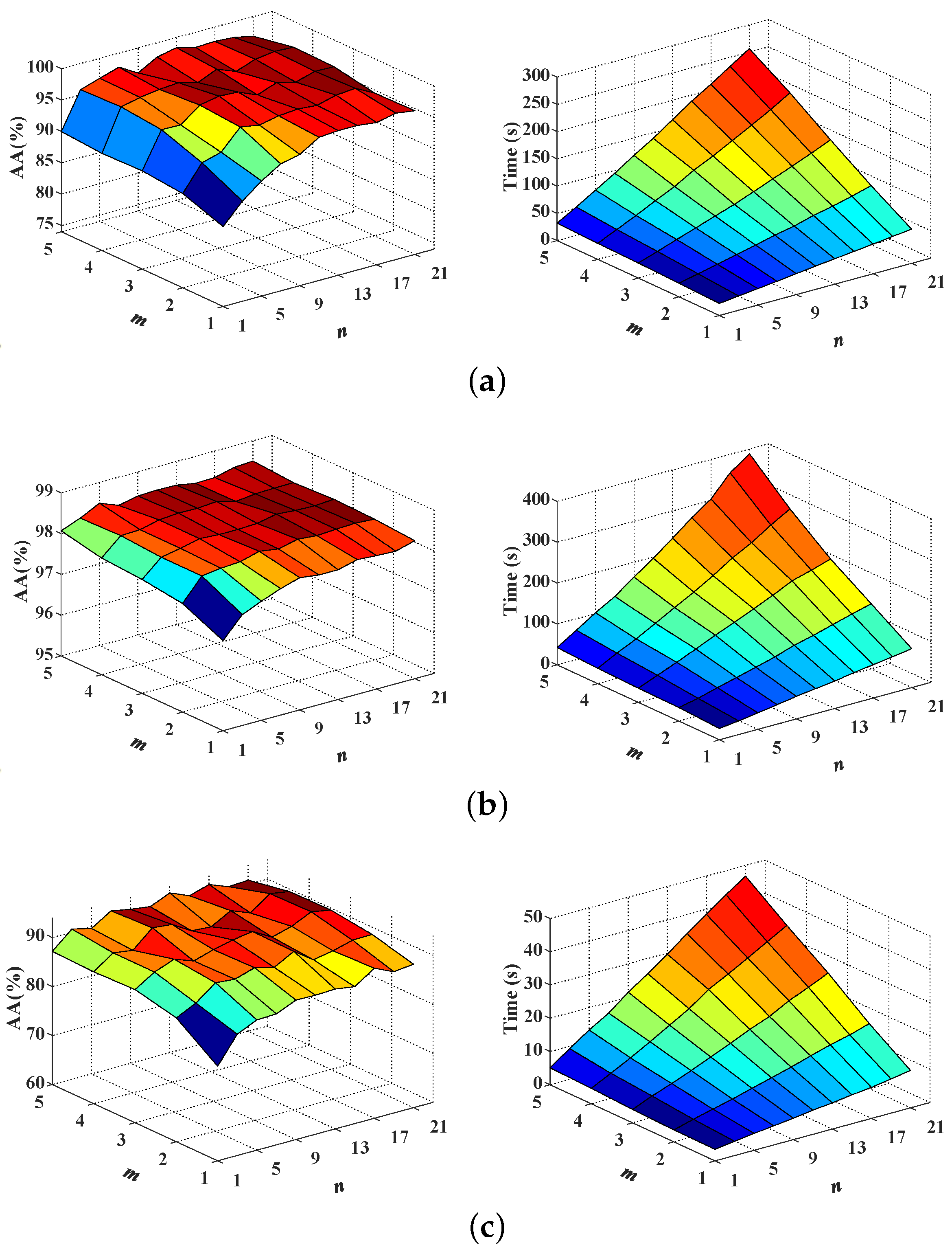
First, the network depth m and width n of MPRN are analyzed together. In our experiments, the m ranges from 1 to 5 with step 1 and n from 1 to 21 with step 2. Consider the fact that extremely shallow networks, compared to deep ones, tend to be difficult in capturing higher level features, which are beneficial for deep semantic feature extraction. However, over-deeper structure will spend great running time. Therefore, a proper network depth should be set to balance classification accuracy against timeliness. As can be observed from the left column of Figure 5, when m and n are respectively larger than 3 and 7, MPRNs achieve relatively stable high accuracy for all data sets, demonstrating the robustness of MPRN to different m and n values. Meanwhile, with m and n values rise, the parameters of the corresponding models and thus the computing time will increase rapidly, as shown in the right column of Figure 5. Therefore, to effectively leverage the overall performance, we set m to 3 for all data sets.

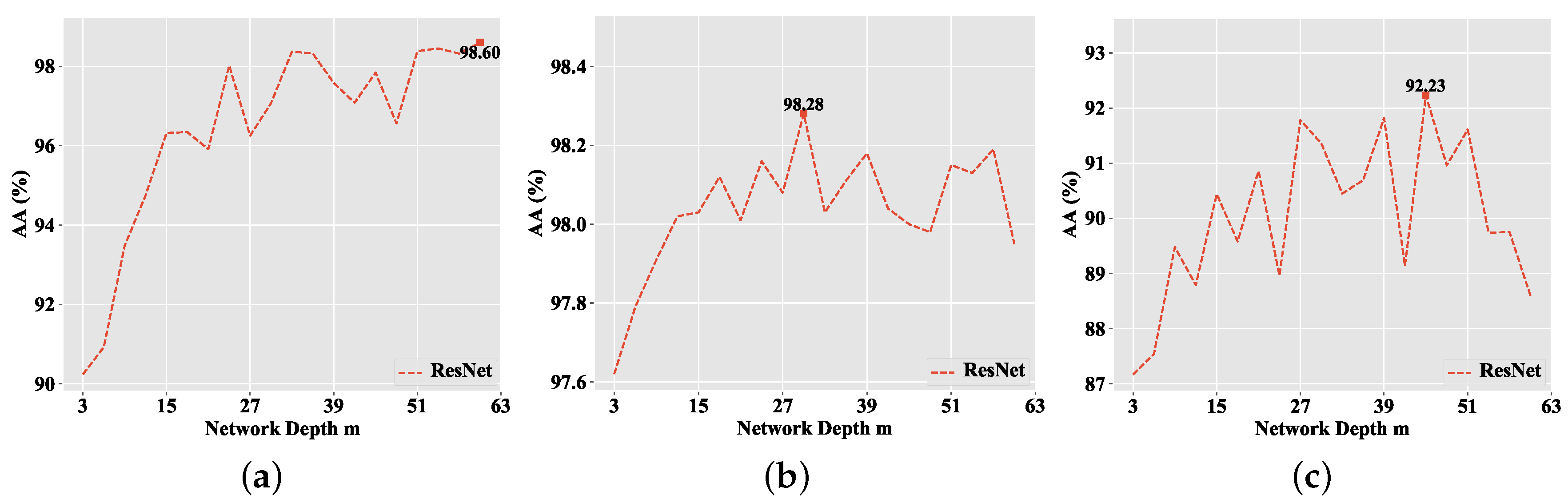
To clearly show the impact of network width n on the classification performance of MPRN, we fix $m=3$ and show the effect of n with value ranging from 1 to 20 with step 1. In addition, we further give a contrastive evaluation of our method with ResNets ($n=1$) with different network depth. To make a fair comparison, for ResNet, the m ranges from 3 to 60 with step 3. In this way, each pair of the MPRN and ResNet have the same number of parameters, for example, MPRN with $m=3$ and $n=9$ has the same number of parameters as ResNet with $m=27$. In addition, when $m=3$ and $n=1$, MPRN and ResNet have the same network architecture.

Figure 6 shows the effects of network width n on the performance (on AA) of the proposed MPRN method over the three data sets, while Figure 7 demonstrates the impacts of network depth m of the ResNet method. From Figure 6 and Figure 7, one can see that increasing any dimension of network, width or depth, will improve classification accuracy. Clearly, when the network depth goes beyond a certain level, increasing the depth become less effective. In contrast, increasing the width can further improve the classification performance.

Table 3. Average accuracy comparison between ResNet and MPRN with different model sizes. The best results are highlighted in bold font.

Data Set	Method	AA	Parameters	(m, n)
Indian Pines	ResNet	98.60%	1.10M	(60, 1)
	MPRN	98.59%	0.35M	(3, 6)
	MPRN	98.73%	0.51M	(3, 9)
Houston University	ResNet	98.28%	0.55M	(30, 1)
	MPRN	98.36%	0.39M	(3, 7)
	MPRN	98.48%	0.98M	(3, 18)
KSC	ResNet	92.23%	0.83M	(45, 1)
	MPRN	92.30%	0.45M	(3, 8)
	MPRN	93.27%	1.04M	(3, 19)

summarizes the optimal network architectures of MPRN and ResNet for each data set. Compared to the ResNet, our MPRN achieves better performance and with fewer parameters on the three data sets. For example, MPRN achieves 98.73% AA with 0.51 M parameters on the Indian Pines data set, while the ResNet achieves 98.60% with 1.10 M parameters. For the Houston University data set, MPRN achieves 98.36% AA with 0.39 M parameters, while the ResNet achieves 98.28% with 0.55 M parameters. For the KSC data set, MPRN achieves 92.30% AA with 0.45 M parameters, while the ResNet achieves 92.23% with 0.83 M parameters. In addition, with the increase of the model size, MPRN obtains better performance (98.48% and 93.27%) on the Houston University and KSC data sets, which further validate the effectiveness of our method. This is because paths in MPRN are relatively shallow, which have significant contribution towards the gradient updates during training. For ResNet, the increase of the depth will not only introduce more deeper paths that do not contribute significant gradient during training but also results in the overfitting phenomenon (see Figure 7b,c). In the following experiments, the optimal architectures of ResNet and MPRN are employed for comparison (see Table 3).

4.4. Comparison Results of Different Methods

The proposed method was compared with several state-of-the-art classification methods available in the literature: (1) 3-D CNN [32]; (2) fully convolutional layer fusion network (FCLFN) [56]; (3) deep feature fusion network (DFFN) [35]; (4) DenseNet [57]; and (5) ResNet [46].

More specifically, 3-D CNN, FCLFN, DFFN, DenseNet, ResNet, together with the proposed MPRN, are spectral-spatial classifiers. 3-D CNN utilizes 3-D convolutional kernels to simultaneously extract the spatial and spectral features from HSIs. FCLFN combines features extracted from each Conv layer for classification. DFFN fuses multiple-layer features from a deep ResNet for classification. DenseNet employs shortcut connections between layers, in which the outputs of the previous layers are concatenated as inputs into all subsequent layers and hence can combine various spectral-spatial features across layers for HSI classification. ResNet is constructed by stacking multiple conventional residual blocks (with a single residual function in each block). In addition, some parameters of the compared methods had been set in advance. For the 3-D CNN, FCLFN, DFFN and DenseNet, the parameters were set according to the default values in the corresponding references. For ResNet and MPRN, the optimal architectures were used according to the Table 3. In addition, they were trained under exactly the same experimental setting, for example, using the same optimizer and L2 weight decay penalty.

The first experiment was conducted on the Indian Pines data set and 10% of the labeled samples in each class were randomly selected for training. The quantitative classification results, that is, classification accuracy of each class, OA, AA, Kappa, F1-score and Precision values obtained by different approaches are reported in

Table 4. Classification accuracies (%) obtained by different methods on the Indian Pines data set. The improvement of MPRN over ResNet is also provided. The best results are highlighted in bold font. In addition, the positive and negative improvements are marked in blue and red, respectively.

Class	Color	3-D CNN [32]	FCLFN [56]	DFFN [35]	DenseNet [57]	ResNet [46]	MPRN	Improvement
1		92.78	92.78	96.67	97.22	98.33	98.89	+0.56
2		98.25	98.77	98.51	99.23	99.28	99.51	+0.23
3		97.17	98.07	97.05	97.77	98.80	98.92	+0.12
4		96.72	99.05	98.52	99.15	98.20	98.52	+0.32
5		96.10	96.47	97.19	97.35	97.97	97.92	–0.05
6		98.87	98.90	98.70	99.28	98.80	99.08	+0.28
7		83.64	74.55	90.91	92.73	100	98.18	–1.82
8		100	99.74	99.58	100	100	100	+0.00
9		96.25	82.50	91.25	98.75	97.50	97.50	+0.00
10		95.28	98.71	97.76	98.43	97.99	98.14	+0.15
11		97.20	98.98	98.93	98.20	99.27	99.38	+0.11
12		96.28	96.66	97.93	97.46	98.35	98.69	+0.34
13		99.39	97.91	98.40	99.75	99.14	98.90	–0.24
14		99.11	99.58	99.72	99.43	99.88	99.98	+0.10
15		97.73	98.51	98.83	99.22	99.55	99.68	+0.13
16		96.71	90.41	90.41	98.90	94.52	96.44	+1.92
OA		97.53	98.47	98.43	98.64	99.01	99.16	+0.15
AA		96.34	95.10	96.90	98.30	98.60	98.73	+0.13
Kappa		97.19	98.25	98.21	98.45	98.87	99.04	+0.17
F1-score		97.53	98.45	98.43	98.64	99.01	99.16	+0.15
Precision		97.58	98.49	98.45	98.66	99.02	99.17	+0.15

. It can be seen that MPRN achieves the best results in terms of the five overall metrics, that is, OA, AA, Kappa, F1-score and Precision. From Table 4, one can observe that MPRN improves the performance of 11 classes out of 16 compared with ResNet, indicating that MPRN is more effective than ResNet. Moreover, the false-color composite image, ground reference map and the classification maps obtained by the six considered methods in a single experiment are shown in Figure 8.

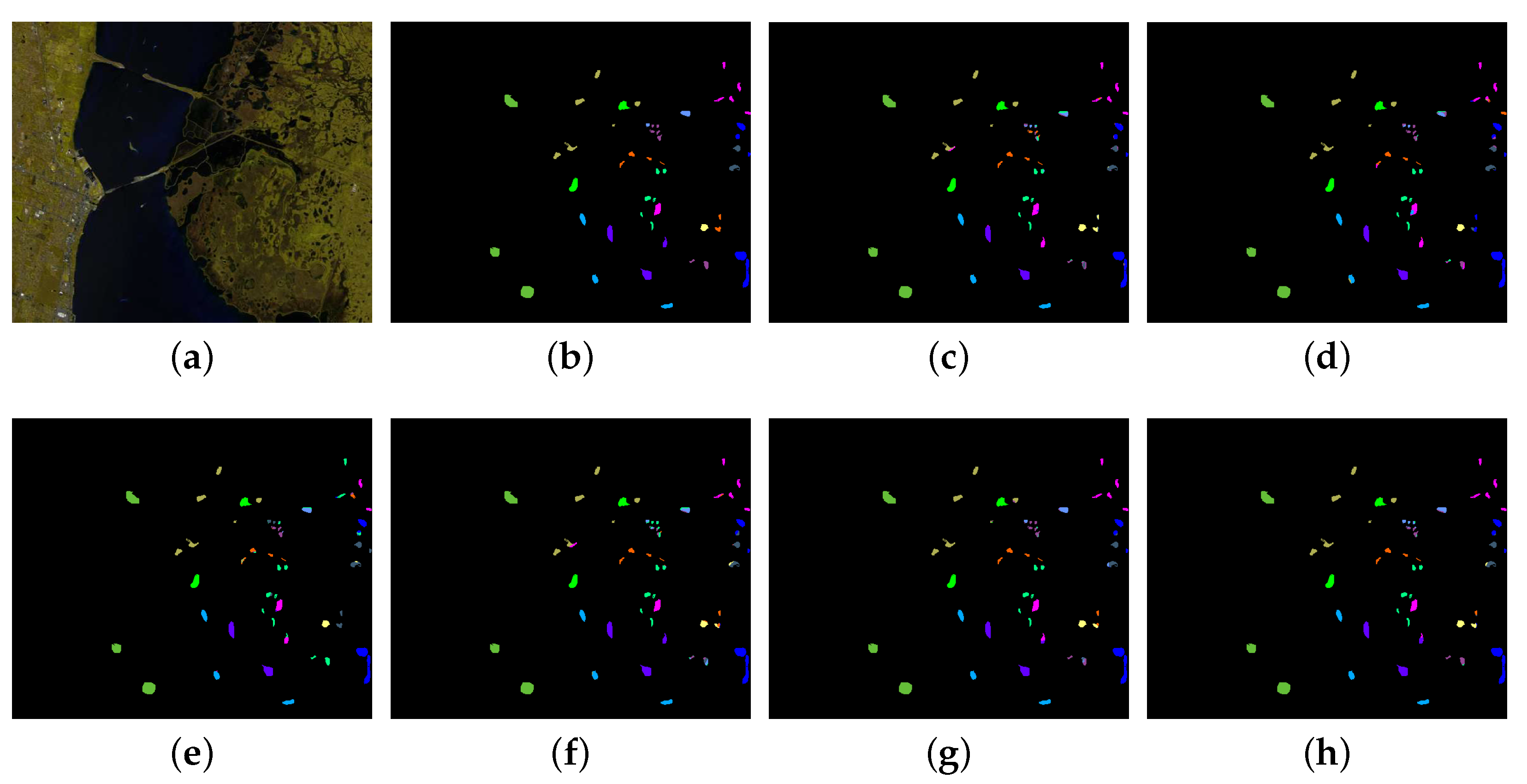
The second and third experiments were conducted on the Houston University and KSC data sets, respectively. For the Houston University data set, 10% of the labeled samples in each class were randomly selected for training. For the KSC data set, 2% of the labeled samples per class were randomly chosen for training.

Table 5. Classification accuracies (%) obtained by different methods on the Houston University data set. The improvement of MPRN over ResNet is also provided. The best results are highlighted in bold font. In addition, the positive and negative improvements are marked in blue and red, respectively.

Class	Color	3-D CNN [32]	FCLFN [56]	DFFN [35]	DenseNet [57]	ResNet [46]	MPRN	Improvement
1		98.80	90.29	95.50	99.38	99.10	99.38	+0.28
2		99.20	97.49	99.26	98.82	99.24	99.42	+0.18
3		99.61	98.64	98.71	99.78	99.61	99.53	–0.08
4		99.13	94.12	94.81	93.06	97.02	99.46	+2.44
5		99.96	99.94	99.86	100	100	100	+0.00
6		93.05	90.04	92.12	91.81	93.59	93.28	–0.31
7		96.27	96.65	96.94	94.00	97.89	97.99	+0.10
8		93.56	95.33	94.47	95.23	97.36	97.65	+0.29
9		96.10	97.40	98.02	94.68	97.36	98.54	+1.18
10		98.67	100	99.84	99.88	99.86	100	+0.14
11		98.40	98.44	99.21	98.91	99.41	99.70	+0.29
12		97.30	98.64	97.46	99.23	98.98	98.92	–0.06
13		92.96	93.28	92.05	91.15	94.72	93.28	–1.44
14		99.88	100	99.77	100	100	100	+0.00
15		99.81	98.52	99.39	100	100	100	+0.00
OA		97.73	96.81	97.44	97.31	98.53	98.88	+0.35
AA		97.51	96.58	97.16	97.06	98.28	98.48	+0.20
Kappa		97.54	96.55	97.24	97.09	98.42	98.79	+0.37
F1-score		97.72	96.81	97.43	97.30	98.53	98.87	+0.34
Precision		97.75	96.90	97.50	97.39	98.56	98.90	+0.34

and

Table 6. Classification accuracies (%) obtained by different methods on the KSC data set. The improvement of MPRN over ResNet is also provided. The best results are highlighted in bold font. In addition, the positive and negative improvements are marked in blue and red, respectively.

Class	Color	3-D CNN [32]	FCLFN [56]	DFFN [35]	DenseNet [57]	ResNet [46]	MPRN	Improvement
1		98.24	98.19	95.14	98.46	99.34	99.73	+0.39
2		66.09	33.56	56.31	81.29	84.29	86.18	+1.89
3		89.67	99.10	93.03	96.48	97.46	99.10	+1.64
4		44.67	57.92	56.83	41.08	85.58	72.50	–13.08
5		32.42	24.05	77.12	36.47	64.31	66.80	+2.49
6		84.93	85.30	82.37	89.22	79.91	96.53	+16.62
7		95.76	89.90	96.97	90.10	100	100	+0.00
8		84.70	80.48	70.94	91.57	98.31	99.95	+1.64
9		84.94	90.04	88.59	95.22	96.06	96.75	+0.69
10		98.08	97.77	98.91	97.41	99.95	99.74	–0.21
11		97.51	100	99.95	98.75	99.60	98.35	–1.25
12		88.44	100	96.84	92.18	94.14	96.92	+2.78
13		99.89	100	100	100	100	100	+0.00
OA		87.91	88.60	89.35	91.04	95.24	96.00	+0.76
AA		81.95	81.25	85.62	85.25	92.23	93.27	+1.04
Kappa		86.54	87.28	88.13	90.02	94.70	95.54	+0.84
F1-score		87.58	87.12	89.19	90.60	95.20	95.94	+0.74
Precision		88.39	88.24	90.60	92.02	95.98	96.38	+0.40

, respectively, show the quantitative classification results obtained by different approaches on the two data sets. It can be seen that the proposed MPRN improves the OA value from 98.53% to 98.88% for the Houston University data set and 95.24% to 96.00% for the KSC data set compared with the ResNet. In addition, the proposed method obtains the best classification performance in terms of the five overall metrics (the OA, AA, Kappa, F1-score and Precision) among all the six methods on the two data sets, which demonstrates the effectiveness of the proposed method. The corresponding classification maps are respectively illustrated in Figure 9 and Figure 10.

As shown in

Table 7. Statistical significance from the standardized McNemar’s test about the difference between methods.

Indian Pines	Houston University	KSC
Z/Significant?	Z/Significant?	Z/Significant?
MPRN vs 3-D CNN
11.42/yes	11.29/yes	19.81/yes
MPRN vs FCLFN
7.45/yes	15.72/yes	19.16/yes
MPRN vs DFFN
7.67/yes	12.96/yes	17.97/yes
MPRN vs DenseNet
6.46/yes	13.66/yes	15.69/yes
MPRN vs ResNet
4.77/yes	6.29/yes	2.86/yes

, the standardized McNemar’s test [58] was performed to demonstrate the statistical significance in accuracy improvement of the proposed MPRN. When the Z value of McNemar’s test is larger than 1.96 and 2.58, it indicates that the difference in accuracy between classifiers 1 and 2 are statistically significant at the 95% and 99% confidence levels, respectively. The Z value larger than 0 means that classifier 1 is more accurate than classifier 2 and vice versa. In this experiment, the proposed MPRN is compared with five other methods, that is, 3-D CNN, FCLFN, DFFN, DenseNet and ResNet. From Table 7, one can see that all the Z values are larger than 2.58, demonstrating that the proposed MPRN can significantly outperform the compared methods.

Finally, the total number of parameters and computing time of the six considered methods on the three data sets are reported in

Table 8. Total number of parameters in different models for the three HSI data sets.

Data Set	3-D CNN	FCLFN	DFFN	DenseNet	ResNet	MPRN
Indian Pines	0.10 M	0.17 M	0.40 M	1.67 M	1.10 M	0.51 M
Houston University	0.07 M	0.17 M	0.40 M	1.66 M	0.55 M	0.98 M
KSC	0.08 M	0.16 M	0.40 M	1.66 M	0.83 M	1.04 M

and

Table 9. Running time (in second) of different methods on the three data sets.

		Indian Pines	Houston University	KSC
3-D CNN	Training	66.21	73.57	6.73
	Test	1.65	1.89	0.88
FCLFN	Training	24.88	36.30	3.96
	Test	0.58	0.80	0.32
DFFN	Training	27.61	40.92	4.94
	Test	0.55	0.82	0.32
DenseNet	Training	61.31	84.75	10.32
	Test	1.33	1.79	0.77
ResNet	Training	182.40	130.46	24.10
	Test	2.45	2.11	1.17
MPRN	Training	73.13	193.91	25.53
	Test	1.38	2.78	1.26

, respectively. From Table 9, we can find that FCLFN achieves the lowest training times on the three data sets. In addition, MPRN spends less time than ResNet on the Indian Pines data set because it has fewer parameters compared with ResNet. For the Houston University and KSC data sets, the proposed method is the most time-consuming, which is attributed to the processing of a large number of Conv layers.

4.5. Effect of Input Spatial Patch Size

In this experiment, we compare our MPRN method with the spatial-spectral ResNet (SSRN) in Reference [37]. In this case, the Indian Pines and KSC data sets are considered. Following Reference [37], 20% of the available labeled samples are randomly selected to form the training set. In addition, input patches with four different spatial sizes {$5\times 5$, $7\times 7$, $9\times 9$ and $11\times 11$} have been considered. Since a patch too large may contain pixels from multiple classes that detract from the target pixel. In addition, it results in the degradation of intersample diversity, increasing the possibility of overfitting and curse of dimensionality as well.

Table 10. Overall accuracy (%) obtained by the proposed MPRN and the spatial-spectral ResNet (SSRN) [37] method when considering different input spatial patch sizes.

	Indian Pines		KSC
Spatial Size	SSRN [37]	MPRN	SSRN [37]	MPRN
$5\times 5$	92.83	99.41	96.99	99.52
$7\times 7$	97.81	99.60	99.01	99.87
$9\times 9$	98.68	99.64	99.51	99.95
$11\times 11$	98.70	99.59	99.57	99.94

shows the overall accuracies obtained in this experiment. From Table 10, one can see that MPRN achieves remarkable improvements in terms of OA regardless of the sizes of the considered image patches. For example, the proposed MPRN reach 6.58 percent higher OA than the SSRN with the same amount of spatial information ($5\times 5$ patch size) on the Indian Pines data set. Furthermore, all the OAs, obtained by MPRN with different patch sizes on the two data sets, are higher than 99%, indicating the robustness of our MPRN method to input patch size.

4.6. Effect of Limited Training Samples

Since manual labeling of hyperspectral data is expensive and time demanding, labeled samples are usually limited in practice. Therefore, it is necessary to assess the performance of the proposed method when limited training data is available. Figure 11 illustrates the overall classification accuracies achieved by different methods on the three data sets using limited numbers of training samples (ranging from 0.1% to 0.5%, with a step of 0.1% per class). As can be seen in Figure 11, for each data set, the proposed MPRN consistently performs the best among all methods under all different training samples, demonstrating the effectiveness and robustness of the proposed approach.

In the face of limited training data, deep networks with a large number of parameters tend to overfit the training set and thus obtain poor accuracy on the testing set. However, MPRN can be interpreted as an ensemble of exponential relatively shallow networks, each of which has a small number of parameters to be optimized and thus avoids the overfitting problem naturally. Therefore, the proposed method is able to provide superior performance when facing limited training data.

5. Conclusions

In this work, a novel network architecture named MPRN is proposed for spectral-spatial HSI classification. The proposed model employs multiple residual functions in the residual blocks in order to make the ResNet wider, rather than deeper. As a result, more shorter-medium neural connections are learned, which can effectively contribute gradient during training. With our analysis, ResNets integrated multiple residual functions in each residual block could achieve better performance than those with much deeper layers and our proposed MPRN, further reduced training parameters, not only achieves comparable or even better performance but spends less operation than ResNet. Experimental results on three real HSI data sets demonstrate that the proposed method performs better than other state-of-the-art methods in terms of both visual performance and quantitative metrics, especially in the face of limited number of training samples.

Note that designing a proper deep learning architecture is important for accurate HSI classification. However, it is a time-consuming and error-prone process. In our future work, neural architecture search methods [59] will be considered to engineer neural architectures in an automatic manner.

References

1. Fang, L.; He, N.; Li, S.; Plaza, A.J.; Plaza, J. A new spatial-spectral feature extraction method for hyperspectral images using local covariance matrix representation. IEEE Trans. Geosci. Remote Sens. 2018, 56, 3534–3546. [Google Scholar] [CrossRef]
2. Yang, X.; Yu, Y. Estimating soil salinity under various moisture conditions: An experimental study. IEEE Trans. Geosci. Remote Sens. 2017, 55, 2525–2533. [Google Scholar] [CrossRef]
3. Zhang, X.; Sun, Y.; Shang, K.; Zhang, L.; Wang, S. Crop classification based on feature band set construction and object-oriented approach using hyperspectral images. IEEE J. Sel. Top. Appl. Earth Obs. Remote Sens. 2016, 9, 4117–4128. [Google Scholar] [CrossRef]
4. Li, J.; Bioucas-Dias, J.M.; Plaza, A. Spectral-spatial classification of hyperspectral data using loopy belief propagation and active learning. IEEE Trans. Geosci. Remote Sens. 2013, 51, 844–856. [Google Scholar] [CrossRef]
5. Ham, J.; Chen, Y.; Crawford, M.M.; Ghosh, J. Investigation of the random forest framework for classification of hyperspectral data. IEEE Trans. Geosci. Remote Sens. 2005, 43, 492–501. [Google Scholar] [CrossRef] [Green Version]
6. Melgani, F.; Bruzzone, L. Classification of hyperspectral remote sensing images with support vector machines. IEEE Trans. Geosci. Remote Sens. 2004, 42, 1778–1790. [Google Scholar] [CrossRef] [Green Version]
7. Li, J.; Bioucas-Dias, J.M.; Plaza, A. Semisupervised hyperspectral image segmentation using multinomial logistic regression with active learning. IEEE Trans. Geosci. Remote Sens. 2010, 48, 4085–4098. [Google Scholar] [CrossRef]
8. Benediktsson, J.A.; Palmason, J.A.; Sveinsson, J.R. Classification of hyperspectral data from urban areas based on extended morphological profiles. IEEE Trans. Geosci. Remote Sens. 2005, 43, 480–491. [Google Scholar] [CrossRef]
9. Camps-Valls, G.; Bruzzone, L. Kernel-based methods for hyperspectral image classification. IEEE Trans. Geosci. Remote Sens. 2005, 43, 1351–1362. [Google Scholar] [CrossRef]
10. Fang, L.; Li, S.; Duan, W.; Ren, J.; Benediktsson, J.A. Classification of hyperspectral images by exploiting spectral-spatial information of superpixel via multiple kernels. IEEE Trans. Geosci. Remote Sens. 2015, 53, 6663–6674. [Google Scholar] [CrossRef]
11. Fang, L.; Li, S.; Kang, X.; Benediktsson, J.A. Spectral-spatial hyperspectral image classification via multiscale adaptive sparse representation. IEEE Trans. Geosci. Remote Sens. 2014, 52, 7738–7749. [Google Scholar] [CrossRef]
12. Fauvel, M.; Tarabalka, Y.; Benediktsson, J.A.; Chanussot, J.; Tilton, J.C. Advances in spectral-spatial classification of hyperspectral images. Proc. IEEE 2013, 101, 652–675. [Google Scholar] [CrossRef]
13. Kang, X.; Li, S.; Benediktsson, J.A. Spectral-spatial hyperspectral image classification with edge-preserving filtering. IEEE Trans. Geosci. Remote Sens. 2014, 52, 2666–2677. [Google Scholar] [CrossRef]
14. Fauvel, M.; Chanussot, J.; Benediktsson, J.A. A spatial–spectral kernel-based approach for the classification of remote-sensing images. Pattern Recognit. 2012, 45, 381–392. [Google Scholar] [CrossRef]
15. Krizhevsky, A.; Sutskever, I.; Hinton, G.E. Imagenet classification with deep convolutional neural networks. In Proceedings of the International Conference on Neural Information Processing Systems (NIPS), Lake Tahoe, NV, USA, 3–6 December 2012; pp. 1097–1105. [Google Scholar]
16. Szegedy, C.; Liu, W.; Jia, Y.; Sermanet, P.; Reed, S.; Anguelov, D.; Erhan, D.; Vanhoucke, V.; Rabinovich, A. Going deeper with convolutions. In Proceedings of the IEEE Conference on Computer Vision and Pattern Recognition (CVPR), Boston, MA, USA, 7–12 June 2015; pp. 1–9. [Google Scholar]
17. Long, J.; Shelhamer, E.; Darrell, T. Fully convolutional networks for semantic segmentation. In Proceedings of the IEEE Conference on Computer Vision and Pattern Recognition (CVPR), Boston, MA, USA, 7–12 June 2015; pp. 3431–3440. [Google Scholar]
18. Sutskever, I.; Vinyals, O.; Le, Q.V. Sequence to sequence learning with neural networks. In Proceedings of the Conference on Advances in Neural Information Processing Systems (NIPS), Montreal, QC, Canada, 8–13 December 2014; pp. 3104–3112. [Google Scholar]
19. Ren, S.; He, K.; Girshick, R.; Sun, J. Faster r-cnn: Towards real-time object detection with region proposal networks. In Proceedings of the Conference on Advances in Neural Information Processing Systems (NIPS), Montreal, QC, Canada, 7–12 December 2015; pp. 91–99. [Google Scholar]
20. Zhang, L.; Zhang, L.; Du, B. Deep learning for remote sensing data: A technical tutorial on the state of the art. IEEE Geosci. Remote Sens. Mag. 2016, 4, 22–40. [Google Scholar] [CrossRef]
21. Li, S.; Song, W.; Fang, L.; Chen, Y.; Ghamisi, P.; Benediktsson, J.A. Deep learning for hyperspectral image classification: An overview. IEEE Trans. Geosci. Remote Sens. 2019. [Google Scholar] [CrossRef]
22. Chen, Y.; Lin, Z.; Zhao, X.; Wang, G.; Gu, Y. Deep learning-based classification of hyperspectral data. IEEE J. Sel. Top. Appl. Earth Obs. Remote Sens. 2014, 7, 2094–2107. [Google Scholar] [CrossRef]
23. Zhong, P.; Gong, Z.; Li, S.; Schönlieb, C.B. Learning to diversify deep belief networks for hyperspectral image classification. IEEE Trans. Geosci. Remote Sens. 2017, 55, 3516–3530. [Google Scholar] [CrossRef]
24. Hu, W.; Huang, Y.; Wei, L.; Zhang, F.; Li, H. Deep convolutional neural networks for hyperspectral image classification. J. Sens. 2015, 2015, 258619. [Google Scholar] [CrossRef]
25. Li, W.; Wu, G.; Zhang, F.; Du, Q. Hyperspectral image classification using deep pixel-pair features. IEEE Trans. Geosci. Remote Sens. 2017, 55, 844–853. [Google Scholar] [CrossRef]
26. Ghamisi, P.; Plaza, J.; Chen, Y.; Li, J.; Plaza, A.J. Advanced spectral classifiers for hyperspectral images: A review. IEEE Geosci. Remote Sens. Mag. 2017, 5, 8–32. [Google Scholar] [CrossRef]
27. He, L.; Li, J.; Liu, C.; Li, S. Recent advances on spectral-spatial hyperspectral image classification: An overview and new guidelines. IEEE Trans. Geosci. Remote Sens. 2018, 56, 1579–1597. [Google Scholar] [CrossRef]
28. Zhang, H.; Li, Y.; Zhang, Y.; Shen, Q. Spectral-spatial classification of hyperspectral imagery using a dual-channel convolutional neural network. Remote Sens. Lett. 2017, 8, 438–447. [Google Scholar] [CrossRef] [Green Version]
29. Fang, L.; Liu, G.; Li, S.; Ghamisi, P.; Benediktsson, J.A. Hyperspectral image classification with squeeze multibias network. IEEE Trans. Geosci. Remote Sens. 2019, 57, 1291–1301. [Google Scholar] [CrossRef]
30. Zhao, W.; Du, S. Spectral-spatial feature extraction for hyperspectral image classification: A dimension reduction and deep learning approach. IEEE Trans. Geosci. Remote Sens. 2016, 54, 4544–4554. [Google Scholar] [CrossRef]
31. Chen, Y.; Jiang, H.; Li, C.; Jia, X.; Ghamisi, P. Deep feature extraction and classification of hyperspectral images based on convolutional neural networks. IEEE Trans. Geosci. Remote Sens. 2016, 54, 6232–6251. [Google Scholar] [CrossRef]
32. Li, Y.; Zhang, H.; Shen, Q. Spectral-spatial classification of hyperspectral imagery with 3D convolutional neural network. Remote Sens. 2017, 9, 67. [Google Scholar] [CrossRef]
33. He, K.; Zhang, X.; Ren, S.; Sun, J. Deep residual learning for image recognition. In Proceedings of the IEEE Conference on Computer Vision and Pattern Recognition (CVPR), Las Vegas, NV, USA, 27–30 June 2016; pp. 770–778. [Google Scholar]
34. Lee, H.; Kwon, H. Going deeper with contextual CNN for hyperspectral image classification. IEEE Trans. Image Process. 2017, 26, 4843–4855. [Google Scholar] [CrossRef]
35. Song, W.; Li, S.; Fang, L.; Lu, T. Hyperspectral image classification with deep feature fusion network. IEEE Trans. Geosci. Remote Sens. 2018, 56, 3173–3184. [Google Scholar] [CrossRef]
36. Mou, L.; Zhu, X.X. Unsupervised spectral-spatial feature learning via deep residual Conv-Deconv network for hyperspectral image classification. IEEE Trans. Geosci. Remote Sens. 2018, 56, 391–406. [Google Scholar] [CrossRef]
37. Zhong, Z.; Li, J.; Luo, Z.; Chapman, M. Spectral-spatial residual network for hyperspectral image classification: A 3-D deep learning framework. IEEE Trans. Geosci. Remote Sens. 2018, 56, 847–858. [Google Scholar] [CrossRef]
38. Paoletti, M.E.; Haut, J.M.; Fernandez-Beltran, R.; Plaza, J.; Plaza, A.J.; Pla, F. Deep pyramidal residual networks for spectral-spatial hyperspectral image classification. IEEE Trans. Geosci. Remote Sens. 2019, 57, 740–754. [Google Scholar] [CrossRef]
39. Wang, L.; Peng, J.; Sun, W. Spatial-spectral squeeze-and-excitation residual network for hyperspectral image classification. Remote Sens. 2019, 11, 884. [Google Scholar] [CrossRef]
40. Veit, A.; Wilber, M.J.; Belongie, S. Residual networks behave like ensembles of relatively shallow networks. In Proceedings of the Conference on Advances in Neural Information Processing Systems (NIPS), Barcelona, Spain, 5–10 December 2016; pp. 550–558. [Google Scholar]
41. Abdi, M.; Nahavandi, S. Multi-residual networks: Improving the speed and accuracy of residual networks. arXiv 2016, arXiv:1609.05672. [Google Scholar]
42. Paoletti, M.E.; Haut, J.M.; Fernandez-Beltran, R.; Plaza, J.; Plaza, A.; Li, J.; Pla, F. Capsule networks for hyperspectral image classification. IEEE Trans. Geosci. Remote Sens. 2019, 57, 2145–2160. [Google Scholar] [CrossRef]
43. Ioffe, S.; Szegedy, C. Batch normalization: Accelerating deep network training by reducing internal covariate shift. In Proceedings of the International Conference on Machine Learning (ICML), Lille, France, 6–11 July 2015; pp. 448–456. [Google Scholar]
44. Srivastava, R.K.; Greff, K.; Schmidhuber, J. Training very deep networks. In Proceedings of the Conference on Advances in Neural Information Processing Systems (NIPS), Montreal, QC, Canada, 7–12 December 2015; pp. 2377–2385. [Google Scholar]
45. Anthony, M.; Biggs, N. Computational Learning Theory; Cambridge University Press: Cambridge, UK, 1997. [Google Scholar]
46. He, K.; Zhang, X.; Ren, S.; Sun, J. Identity mappings in deep residual networks. In Proceedings of the European Conference on Computer Vision (ECCV), Amsterdam, The Netherlands, 8–16 October 2016; pp. 630–645. [Google Scholar]
47. Simonyan, K.; Zisserman, A. Very deep convolutional networks for large-scale image recognition. arXiv 2014, arXiv:1409.1556. [Google Scholar]
48. Zagoruyko, S.; Komodakis, N. Wide residual networks. arXiv 2016, arXiv:1605.07146. [Google Scholar]
49. He, K.; Zhang, X.; Ren, S.; Sun, J. Delving deep into rectifiers: Surpassing human-level performance on imagenet classification. In Proceedings of the IEEE Conference on Computer Vision and Pattern Recognition (CVPR), Santiago, Chile, 7–13 December 2015; pp. 1026–1034. [Google Scholar]
50. Kingma, D.P.; Ba, J.L. Adam: A method for stochastic optimization. In Proceedings of the International Conference on Learning Representations (ICLR), San Diego, CA, USA, 7–9 May 2015. [Google Scholar]
51. Hyperspectral Remote Sensing Scenes. Available online: http://www.ehu.eus/ccwintco/index.php?title=Hyperspectral_Remote_Sensing_Scenes (accessed on 30 July 2019).
52. 2013 IEEE GRSS Data Fusion Contest. Available online: http://www.grss-ieee.org/community/technical-committees/data-fusion/2013-ieee-grss-data-fusion-contest/ (accessed on 30 July 2019).
53. Vihinen, M. How to evaluate performance of prediction methods? Measures and their interpretation in variation effect analysis. BMC Genomics 2012, 13, S2. [Google Scholar] [CrossRef]
54. Loshchilov, I.; Hutter, F. Sgdr: Stochastic gradient descent with warm restarts. arXiv 2016, arXiv:1608.03983. [Google Scholar]
55. Paszke, A.; Gross, S.; Chintala, S.; Chanan, G.; Yang, E.; DeVito, Z.; Lin, Z.; Desmaison, A.; Antiga, L.; Lerer, A. Automatic Differentiation in Pytorch. Available online: https://pytorch.org/ (accessed on 13 July 2019).
56. Zhao, G.; Liu, G.; Fang, L.; Tu, B.; Ghamisi, P. Multiple convolutional layers fusion framework for hyperspectral image classification. Neurocomputing 2019, 339, 149–160. [Google Scholar] [CrossRef]
57. Paoletti, M.; Haut, J.; Plaza, J.; Plaza, A. Deep&dense convolutional neural network for hyperspectral image classification. Remote Sens. 2018, 10, 1454. [Google Scholar]
58. Foody, G.M. Thematic map comparison: Evaluating the statistical significance of differences in classification accuracy. Photogramm. Eng. Remote Sens. 2004, 70, 627–633. [Google Scholar] [CrossRef]
59. Elsken, T.; Metzen, J.H.; Hutter, F. Neural architecture search: A survey. arXiv 2018, arXiv:1808.05377. [Google Scholar]
Figure 1. Architecture of a residual block.
Remotesensing 11 01896 g001
Figure 2. Illustration of a 3-block ResNet. (a) The conventional representation based on Equation (5). (b) The unraveled view with 2 3 implicit paths connecting input to output based on Equation (6). Circular nodes denote additions.
Remotesensing 11 01896 g002
Figure 3. Different residual block architectures. (a) Original residual block containing one residual function. (b) Multipath residual block consisting of multiple residual functions.
Remotesensing 11 01896 g003
Figure 4. Framework of multipath ResNet (MPRN) for hyperspectral image (HSI) classification.
Remotesensing 11 01896 g004
Figure 5. Classification performance and execution time of MPRN with different m and n values on the (a) Indian Pines, (b) Houston University, and (c) KSC data sets.
Remotesensing 11 01896 g005
Figure 6. The average accuracy of MPRN with various network width n on the (a) Indian Pines, (b) Houston University and (c) KSC data sets.
Remotesensing 11 01896 g006
Figure 7. The average accuracy of ResNet with various network depth m on the (a) Indian Pines, (b) Houston University, and (c) KSC data sets.
Remotesensing 11 01896 g007
Figure 8. Indian Pines data set. (a) False-color composite image. (b) Ground reference map. The classification maps obtained by the (c) 3-D convolutional neural network (CNN) (97.53), (d) fully convolutional layer fusion network (FCLFN) (98.47), (e) deep feature fusion network (DFFN) (98.43), (f) DenseNet (98.64), (g) ResNet (99.01) and (h) MPRN (99.16). Note that the overall classification accuracies (in %) are shown in brackets.
Remotesensing 11 01896 g008
Figure 9. Houston University data set. (a) False-color composite image. (b) Ground reference map. The classification maps obtained by the (c) 3-D CNN (97.73), (d) FCLFN (96.81), (e) DFFN (97.44), (f) DenseNet (97.31), (g) ResNet (98.53) and (h) MPRN (98.88). Note that the overall classification accuracies (in %) are shown in brackets.
Remotesensing 11 01896 g009
Figure 10. KSC data set. (a) False-color composite image. (b) Ground reference map. The classification maps obtained by the (c) 3-D CNN (87.91), (d) FCLFN (88.60), (e) DFFN (89.35), (f) DenseNet (91.04), (g) ResNet (95.24) and (h) MPRN (96.00). Note that the overall classification accuracies (in %) are shown in brackets.
Remotesensing 11 01896 g010
Figure 11. Overall classification accuracies (in %) obtained by 3-D CNN [32], FCLFN [56], DFFN [35], DenseNet [57], ResNet [46] and MPRN when considering different percentages of training samples on the (a) Indian Pines, (b) Houston University and (c) KSC data sets.
Remotesensing 11 01896 g011