Abstract
The integration of different remote sensing datasets acquired from optical and radar sensors can improve the overall performance and detection rate for mapping sub-surface archaeological remains. However, data fusion remains a challenge for archaeological prospection studies, since remotely sensed sensors have different instrument principles, operating in different wavelengths. Recent studies have demonstrated that some fusion modelling can be achieved under ideal measurement conditions (e.g., simultaneously measurements in no hazy days) using advance regression models, like those of the nonlinear Bayesian Neural Networks. This paper aims to go a step further and investigate the impact of noise in regression models, between datasets obtained from ground-penetrating radar (GPR) and portable field spectroradiometers. Initially, the GPR measurements provided three depth slices of 20 cm thickness, starting from 0.00 m up to 0.60 m below the ground surface while ground spectral signatures acquired from the spectroradiometer were processed to calculate 13 multispectral and 53 hyperspectral indices. Then, various levels of Gaussian random noise ranging from 0.1 to 0.5 of a normal distribution, with mean 0 and variance 1, were added at both GPR and spectral signatures datasets. Afterward, Bayesian Neural Network regression fitting was applied between the radar (GPR) versus the optical (spectral signatures) datasets. Different regression model strategies were implemented and presented in the paper. The overall results show that fusion with a noise level of up to 0.2 of the normal distribution does not dramatically drop the regression model between the radar and optical datasets (compared to the non-noisy data). Finally, anomalies appearing as strong reflectors in the GPR measurements, continue to provide an obvious contrast even with noisy regression modelling.
1. Introduction
The detection of sub-surface buried targets remains a challenge for different disciplines such as archaeological prospection [1,2,3]; forensic archaeology [4,5,6]; urban planning (e.g., pipe detection) [7,8,9]; military and security purposes (e.g., land-mines) [10,11].
Detection of archaeological remains is usually achieved based on the exploitation of remote sensing sensors. As a non-destructive tool, remote sensing technology offers several advantages to researchers, including fast prospecting and mapping, acquisition of digital geospatial information, and a multi-scale coverage from a local to a regional level.
The traditional ways of mapping archaeological remnants have long been shifted from trench excavations to multi-sensor prospection providing evidence of the cultural context in the shallow depths [12,13,14]. Indeed, the use of multi-source datasets is quite familiar in the area of archaeological prospection offering new technologies for the detection of sub-surface archaeological remains [15,16,17,18]. However, the current integration of the different prospection results as those obtained from spaceborne, airborne and ground sensors is analysed in a Geographical Information System (GIS) environment through the superposition of the various thematic layers [19,20,21].
The fusion of the different outcomes from remote sensors can assist in a better understanding of the sub-surface space. Fusion based on dissimilar datasets may not only increase the detection accuracy of the sub-surface anomalies, but it can also improve the detection performance with respect to recall and precision. However, as Opitz and Herrmann [22] and Leisz [23] argue, the fusion of archaeological prospection multi-sensor datasets is quite promising but still remains a challenge for the scientific community to address in the future. In the last couple of years, studies have shown that the fusion of different prospection datasets can be achieved using advanced regression models. For instance, local regression models between different ground geophysical prospection datasets including ground-penetrating radar, magnetic gradiometry and electrical resistivity have been investigated, demonstrating that “…high correlation frequently correspond with robust anomalies observed in each data set and offer objective criteria for assessments of correlation” [24]. The integration of optical and radar ground sensors has also been investigated in the recent past [25,26]. The results of these studies showed that some correlation between heterogenous remotely sensed datasets does exist, addressing thus the paradox between theory and correlational studies, as it has been also argued by Kvamme [24].
This paper aims to go a step further, building upon the work initially performed and presented at Sarris et al. [27] and then by Agapiou et al. [25,26]. In those studies, various regression models, both simple and advanced, have been investigated in order to assess the correlation strength (Pearson coefficient r) between GPR datasets (used as depth slices of 20 cm) and ground hyperspectral signatures covering both the visible and the near-infrared part of the spectrum. The analysis was carried out using more than 71 different optical products (mainly multispectral and hyperspectral vegetation indices), which were correlated with the different GPR depth slices (i.e., 0.00–0.20; 0.20–0.40 and 0.40–0.60 m depth slices). The overall results have shown that a high global correlation r of up to 0.70 can be achieved between the optical and radar data using non-linear Bayesian Neural Network regression fitting models.
However, in those studies, the in-situ ground measurements were collected under ideal conditions since both the GPR and the spectroradiometer sensors were simultaneously recording in a cloud-free, non-hazy day with a low level of humidity. So, the critical question raised is whether the correlation values reported by Agapiou and Sarris [25] would remain the same if the acquisition of ground datasets were performed under different scenarios (e.g., data collected separately with different meteorological and environmental conditions).
In order to understand the impact of noise, which can be generated from both environmental and meteorological factors, as well as from noise that is inherent in the sensors’ sensitivity, we proceed to a simulation of the regression model with added noise in raw optical and radar datasets. Specifically, random noise following a Gaussian normal distribution was added to the GPR and the spectroradiometric measurements prior to their regression modelling. This study, therefore, is carried out on a theoretical and simulation basis, aiming to give us some insights on how potential noise can impact fusion modelling. The random noise was gradually increased to both optical and radar datasets (which were used also by Agapiou and Sarris [25]) followed by a Bayesian Neural Network regression model.
The paper presents the overall methodology adopted as well as the results obtained from the various simulations working with noisy data. Initially, a short description of the case study area and the datasets are presented, following by the methodology section. Then the overall results of this simulation study are provided, following by a general discussion on the key findings of the study.
2. Case Study Area and Datasets
2.1. Case Study Area
One of the Hungarian National Parks, namely the Vésztő-Mágor Tell, situated in the southeastern Great Hungarian Plain, was selected as the case study (Figure 1). The site, which approximately covers 4.25 hectares at a height of 9 m a.s.l., was investigated in the previous years as part of the Körös Regional Archaeological Project [28] with various non-invasive techniques including magnetics, GPR, electrical resistivity tomography (ERT) and Electromagnetic induction (EMI) methods. Previous excavations during the 1970s and 1980s revealed that the area was initially settled by Szakálhát culture farmers during the late Middle Neolithic period, while the area was systematically occupied until the Late Neolithic period (c. 5000–4600 B.C. calibrated). On top of this stratigraphy, the layers found suggests the abandonment of the site until the formation of an Early Copper Age settlement and later on by a Middle Copper Age settlement. During the 11th century AD, a church followed by a monastery was established on top of the Tell. After various modifications and reconstructions, the monastery was destroyed during the early 19th century. Currently, in addition to the archaeological museum located within the historic wine cellar, the 1986 excavation trench can be seen with several features from different periods remaining in situ. More information regarding the archaeological context of the Vésztő-Mágor Tell can be found in [29,30,31,32,33].
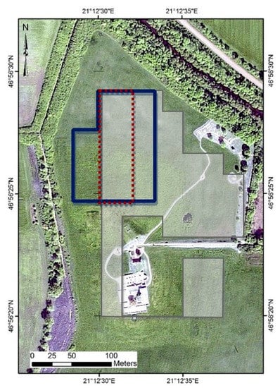
Figure 1.
Area covered from the different techniques: Grey and blue polygons indicate the areas covered from the geophysical surveys (magnetic and GPR survey, respectively), the red polygon indicates the area covered from the ground spectroradiometric measurements (Latitude: 46°56′24.36″; Longitude: 21°12′32.67″) (source [26]).
2.2. Data Sources
In the last phases of the Körös Regional Archaeological Project (KRAP), which was directed by William A. Parkinson of the Department of Anthropology, The Field Museum of Chicago, and Attila Gyucha of the Field Service of Cultural Heritage, Hungary, two different ground prospection methods were implemented in addition to the previous ground-based prospection techniques. The first one was a traditional GPR survey using a Noggin Plus (Sensors & Software, Ontario, Canada) GPR with a 250 MHz antenna while the second method was based on a portable field spectroradiometer, namely the GER-1500 spectroradiometer (Spectra Vista Corporation, New York, NY, USA), with a spectral range of 350–1050 nm. The area of measurements is shown in Figure 1 above. The red polygon indicates the area covered from the ground spectroradiometric measurements while the blue polygon indicates the areas covered from the GPR geophysical survey.
3. Methodology
The overall methodology of this study is presented in Figure 2. Both spectroradiometric and GPR measurements were collected moving along parallel transects 0.5 m apart, with 5 cm sampling along the lines for the GPR, covering an area of 20 × 90 m (1800 square meters). The data have been collected simultaneously to eliminate the influence of noise from other external factors (mainly climatic changes and variation of soil conditions, such as humidity). Once the data collection was accomplished, pre-processing steps including noise removal and filtering were applied. Then depth slices of 20 cm thickness were produced from the GPR datasets. The ground spectroradiometric measurements were resampled to multispectral bands (blue; green; red; near-infrared) using a relative spectral response (RSR) filter (see Equation (1)). The RSR filters define the instrument’s relative sensitivity to radiance in various parts of the electromagnetic spectrum. RSR filters have a value range from 0 to 1 and are unit-less since they are relative to the peak response.
where Rband = reflectance at a range of wavelength (e.g., blue band); Ri = reflectance at a specific wavelength (e.g., R450 nm) and RSRi = relative response value at the specific wavelength. Based on the multispectral bands and the hyperspectral bands of the spectroradiometer, more than 65 hyperspectral and multispectral indices were calculated. The overall equations and references of the vegetation indices can be found in Appendix A.

Figure 2.
Overall methodology followed in this study.
From previous studies [25,26], the first three depth slices (i.e., 0.00–0.20; 0.20–0.40 and 0.40–0.60 m below ground surface) were correlated with the optical products taken from the spectroradiometer (i.e., vegetation indices). Depths beyond the 0.60 m below ground surface did not provide any reliable results [25]. More details regarding data processing can be found in [25,26].
In our example, a randomly normally distributed noise of a standard deviation of 0.1; 0.2; 0.3; 0.4 and 0.5 (hereafter referred as the noise of level 0.1; 0.2; 0.3; 0.4 and 0.5 respectively) was gradually added at the three GPR depth slices and the vegetation indices. Various assessments were carried out based on all levels of noise aiming to understand the correlation performance of the radar datasets against the optical products. This correlation, as mentioned earlier, was based on the Bayesian Neural Network regression fitting, following the same procedure as in Agapiou and Sarris [25].
The neural network fitting was processed by the MathWorks MATLAB R2016b software. The Bayesian Neural Network is a neural network with a prior distribution on its weights, where the likelihood for each data is given by Equation (2).
where NN is a neural network whose weights and biases originate from the latent variable w [34]. From the whole dataset, 85% was used for training purposes while the remaining 15% was used for testing the fusion models. The results from the above regression were compared against the real GPR datasets and the non-noisy regression models.
4. Results
The various results produced during this study are presented below. The results are grouped into four categories for better interpretation. Section 4.1 presents the impact of the random noise added at the multispectral bands regressed against the GPR depth slices. The next section (Section 4.2) includes the results from the regression models between the multispectral bands against the noisy GPR depth slices (from 0.00 to 0.60 m), while the impact of the random noise added at both multispectral bands and the GPR depth slices are presented in Section 4.3. Finally, the impact of the random noise added to vegetation indices against the GPR depth slices is demonstrated in Section 4.4.
4.1. Random Noise at Spectral Bands
Normally distributed random noise with a standard deviation of 0.1; 0.2; 0.3; 0.4 and 0.5 was added in the four multispectral bands (Band 1: Blue; Band 2: Green; Band 3: Red and Band 4: Near-infrared) after the use of the RSR filters as shown in Figure 3. Column (a) shows the initial spectral bands as extracted from the spectroradiometric campaigns following a kriging interpolation method. Column (a) is considered in this case as the ground truth dataset for comparison purposes. Columns (b) to (f) shows the multispectral bands after the inclusion of the random noise starting from a level of 0.1 up to 0.5, respectively. The first row of Figure 3 shows the results for the first band (blue), while the second (green), third (red) and the fourth (near-infrared) bands are demonstrated on the second, third and fourth rows of Figure 3, respectively. It is obvious that the noise added in the spectral bands alters the final interpretation compared to the truth datasets (Column (a)), especially in the near-infrared part of the spectrum (see 4th row). However, strong anomalies—as depicted from the spectroradiometer—as those observed at around 80 m on the north axis (see the arrow of Figure 3) are still visible even in datasets with a high level of noise.
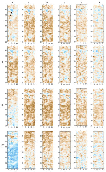
Figure 3.
Column a: Reflectance of spectral bands; Column b: Reflectance of spectral bands with random noise of level 0.1 of the standard normal distribution; Column c: Reflectance of spectral bands with random noise of level 0.2 of the standard normal distribution; Column d: Reflectance of spectral bands with random noise of level 0.3 of the standard normal distribution; Column e: Reflectance of spectral bands with random noise of level 0.4 of the standard normal distribution; Column f: Reflectance of spectral bands with random noise of level 0.5 of the standard normal distribution. Row I: Blue band (Band 1); Row II: Green band (Band 2); Row III: Red band (Band 3) and Row IV: Near Infrared (NIR) band (Band 4).
Preliminary coring results suggest that such linear anomalies, like those observed in Figure 3 (see black arrow) should be linked with ditches, while some of them (not shown here) may exceed 4 m in depth. Structural similarities with other Neolithic fortifications led archaeologists to suspect that part of the ditch and palisade system at the Vésztő-Mágor Tell was established during this period [28].
In order to quantify the impact of the added noise to the regression model, all four multispectral bands (in all levels of noise, including level 0—noiseless) were regressed separately against the three GPR depth slices. The Pearson regression value (r), as well as the relative Mean Square Error (MSE) compared with level 0 (noiseless datasets), used in the next sections, are criteria of the regression performance and are presented in Equations (3) and (4), respectively:
where x is the observed GPR-measurement, y is the BNN modelled GPR result, and n is the total number of measurements.
Figure 4a shows the results of the Pearson regression value and Figure 4b the results from the MSE analysis. We can observe that the added noise decreases steadily the correlation value r while in contrary the MSE increases progressively for all depth slices. The correlation coefficient r falls from over 0.50 to 0.20 at the noisiest datasets for the first depth slice (0.00–0.20 m), from 0.42 to 0.09 for the second depth slice (0.20–0.40 m) and from 0.49 to 0.28 for the third depth slice (0.40–0.60 m). Noisiest datasets of spectral bands (0.4 and 0.5) provide even less correlation coefficient values for all depth slices. The MSE increases up to 20% for the level of 0.3 of random noise while beyond that level of noise (i.e., levels 0.4 and 0.5) the MSE increases significantly. Results of the MSE for the normally distributed random noise with a standard deviation of 0.4 and 0.5 are not shown since their performance was considered very poor (r lower than 0.10).
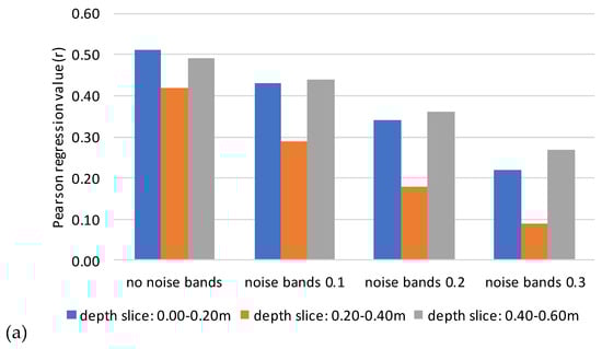
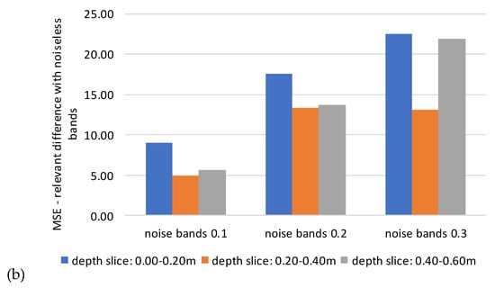
Figure 4.
(a) Pearson regression value (r) of the fusion between the ground-penetrating radar (GPR) depth slices and the four bands based on the Bayesian Neural Network. (b) Relative difference (%) of the Mean Square Error (MSE) of the noisy data of 0.1–0.3 standard deviation against the noiseless datasets. GPR depth slice of 0.00–0.20 m is shown with blue color, depth slice of 0.20–0.40 m with an orange color and depth slice 0.40–0.60 m depth slice with a gray color.
4.2. Random Noise at GPR Depth Slices
In a similar way as before, the Bayesian Neural Network correlation was applied after adding random noise only to the GPR depth slices. Column (a) of Figure 5, shows the initial raw GPR data (noiseless datasets), while the rest of the columns (b to f) shows the simulated GPR depth slices with a noise level from 0.1 to 0.5, respectively. Results from the depth slice 0.00–0.20 m are demonstrated in the first row, while the depth slices 0.20–0.40 and 0.40–0.60 m are shown in the second and third-row correspondingly. From the visual interpretation of the results, it becomes evident that noise of levels 0.1 and 0.2 share similar patterns of anomalies as the one depicted at the original datasets (see first column of Figure 5, noiseless GPR depth slices), while noise beyond the level of 0.2 saturates the overall GPR signal. However, once again, the strong linear anomaly at around 80 m on the y-axis remains visible in all levels of noise (see arrow in Figure 5).
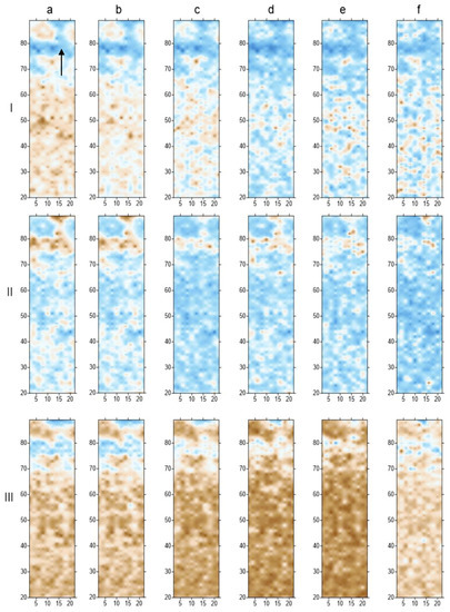
Figure 5.
Column a: Raw GPR data; Column b: GPR data with random noise of level 0.1 of the standard normal distribution; Column c: GPR data with random noise of level 0.2 of the standard normal distribution; Column d: GPR data with random noise of level 0.3 of the standard normal distribution; Column e: GPR data with random noise of level 0.4 of the standard normal distribution; Column f: GPR data with random noise of level 0.5 of the standard normal distribution. Row I: Depth slice of 0.00–0.20 m below ground surface; Row II: Depth slice of 0.20–0.40 m below ground surface and Row III: Depth slice of 0.40–0.60 m below ground surface.
Figure 6 shows the statistics from this Bayesian Neural Network regression fitting of the multispectral bands against the GPR depth slices (with and without noise). The results are shown once again in relation to the Pearson correlation coefficient (r) and the relative MSE in terms of percentage compared with the noiseless datasets. The correlation analysis shows a comparable trend as observed in the previous experiment (see Section 4.1; Figure 4): the correlation coefficient value drops gradually with the increase of noise for all depth slices, having similar linear trend, while the MSE increases exponentially with the increase of noise level. It should be mentioned that for noise levels 0.1 and 0.2 the correlation coefficient decreases slightly from 0.50 to 0.40 for the first depth slice, from 0.42 to 0.38 for the second depth slice and from 0.48 to 0.46 for the third depth slice. Even though MSE for these depth slices increases, it is worth to notice the large difference in the MSE between the first depth slice (0.00–0.20m) and the rest of the depth slices.
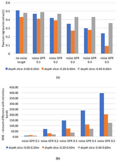
Figure 6.
(a) Pearson regression value (r) of the fusion between the GPR depth slices and the four bands based on the Bayesian Neural Network. (b) Relative difference (%) of the Mean Square Error (MSE) of the noisy data of 0.1–0.5 standard deviation against the noiseless datasets. GPR depth slice of 0.00–0.20 m is shown with blue color, depth slice of 0.20–0.40 m with an orange color and depth slice 0.40–0.60 m depth slice with a gray color.
4.3. Random Noise at Spectral Bands and GPR Depth Slices
Afterward, random noise was added at both multispectral bands and the GPR depth slices starting from level 0.1 and increasing by 0.1 until the level of 0.5. Again, the (noisy) spectral bands were set as inputs and the (noisy) GPR depth slices were set as targets in the Bayesian Neural Network regression fitting models. Once the correlation was estimated then the optical data (i.e., spectral bands) were simulated as GPR depth slices as shown in Figure 7.

Figure 7.
Column a-I: Raw GPR data at depth slice of 0.00–0.20 m below ground surface; a-II: Raw GPR data at depth slice of 0.20–0.40 m below ground surface; a-III: Raw GPR data at depth slice of 0.40–0.60 m below ground surface; b-I: Simulated GPR data at depth slice of 0.00–0.20 m below ground surface with 0.1 noise at spectral band and 0.1 noise at raw GPR data; b-II: Simulated GPR data at depth slice of 0.20–0.40 m below ground surface with 0.1 noise at spectral band and 0.1 noise at raw GPR data; b-III: Simulated GPR data at depth slice of 0.40–0.60 m below ground surface with 0.1 noise at spectral band and 0.1 noise at raw GPR data; c-I: Simulated GPR data at depth slice of 0.00–0.20 m below ground surface with 0.2 noise at spectral band and 0.1 noise at raw GPR data; c-II: Simulated GPR data at depth slice of 0.20–0.40 m below ground surface with 0.2 noise at spectral band and 0.1 noise at raw GPR data and c-III: Simulated GPR data at depth slice of 0.40–0.60 m below ground surface with 0.2 noise at spectral band and 0.1 noise at raw GPR data.
Column (a) of Figure 7 shows the raw GPR data at the depth slice of 0.00–0.20; 0.20–0.40 and 0.40–0.60 m below ground surface. Column (b) of Figure 7, shows the simulated GPR data (from the optical data) at depth slice of 0.00–0.20, 0.20–0.40 and 0.40–0.60 m below ground surface with the noise of level 0.1. The last column (c) of Figure 7, shows the simulated results as before, with a noise level of 0.2. The most interesting result from Figure 7 is that the linear anomaly that is depicted in all depth slices (see arrow in Figure 7) continues to be visible. The high contrast of this linear anomaly is noticeable in all scenarios, even with a noise level of 0.2, allowing thus to suggest that some correlation could be achieved for strong anomalies, even in cases where no ideal conditions of measurements are feasible.
The overall statistics from the above-mentioned analysis are shown in Figure 8. The correlation coefficient value r ranges for noise level 0.1 from 0.30 up to 0.45 for all depth slices. However, the correlation coefficient value r decreases even further for the noisiest datasets (level of 0.2 at spectral bands and level 0.1 at the GPR depth slices). The correlation achieved by Agapiou and Sarris [25] is shown as with a dot in Figure 8 for each depth slice. The difference achieved in the correlation using the truth data (indicated with dots) and the noisy datasets of level 0.2 is obvious in Figure 8.

Figure 8.
Pearson regression value (r) of the fusion between the noisy GPR depth slices (level of 0.1) and the noisy spectral bands (level 0.1 and 0.2) based on the Bayesian Neural Network. GPR depth slice of 0.00–0.20 m is shown with blue color, depth slice of 0.20–0.40 m with an orange color and depth slice 0.40–0.60 m depth slice with a gray color. Correlation achieved with the noiseless dataset is shown with dots for each depth slice.
4.4. Random Noise and Vegetation Indices
Even though a moderate correlation coefficient r was achieved in the previous experiments, these results are aligned with the outcomes presented by Agapiou and Sarris [15]. The correlation is expected to increase once we use vegetation indices (both multispectral and hyperspectral indices) in the regression model. For this reason, the regression analysis was extended by analyzing the correlation performance against the (a) NDVI, (b) 13 multispectral and (c) 53 hyperspectral indices, listed in Table A1 and Table A2 (Appendix A).
The results of the regression modelling between the NDVI, the multispectral and hyperspectral indices against all the noisy GPR depth slices of level 0.1 and level 0.2 are shown in Figure 9a,b, respectively. The correlation coefficient score is much higher—up to 0.61—compared to the previous outcomes discussed in Section 4.1, Section 4.2 and Section 4.3. As in earlier studies (see [25,26]), the hyperspectral indices tend to provide the highest correlation coefficient values ranging from 0.50–0.60 for all depth slices. The regression score slightly decreases in the noisiest datasets (Figure 9b) for all combinations of correlation.
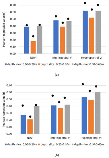
Figure 9.
Pearson regression value (r) of fusion between the (a) noisy GPR depth slices of level 0.1 and (b) noisy GPR depth slices level 0.2 for a depth slice of 0.00–0.20 (blue color), 0.20–0.40 (orange color) and 0.40–0.60 m (gray color). The regression model was tested between the noisy GPR depth slices against the (i) NDVI, (ii) 13 multispectral vegetation indices and (iii) 53 hyperspectral vegetation indices (see details for multispectral and hyperspectral indices in Table A1 and Table A2 respectivelly, Appendix A). Correlation achieved with the noiseless dataset is shown with a dot for each depth slice.
A similar experiment was also carried out with noisy multispectral bands of levels 0.1 and 0.2, which subsequently were used to estimate 13 multispectral indices (see Table A1, Appendix A). The added noise dropped the correlation coefficient value from 0.50 to 0.40 and then to 0.35 for the first depth slice, 0.42 to 0.38 and then to 0.18 for the second depth slice and 0.50 to 0.44 and then to 0.38 for the last depth slice, as estimate for noiseless, level 0.1 and level 0.2 noise, respectively. The overall results are quite similar to the correlation achieved by Agapiou and Sarris [25] and illustrated as dots in Figure 10. This allows us to assume that the impact of noise up to a level of 0.2 does not dramatically change the correlation fitting score (r) between the optical and the radar datasets.

Figure 10.
Pearson regression value (r) of fusion between the GPR depth slices against the 13 multispectral vegetation indices (with and without noise) (see details for multispectral indices in Table A1, Appendix A). Correlation achieved with the noiseless dataset is shown with a dot for each depth slice.
5. Discussion
As was expected, the added noise to the datasets changed the overall regression fitness of the models. The previous section provided four different examples of how random noise may influence the overall regression between the radar and the optical ground datasets. The overall findings suggest that fusion between diverse datasets, as those described here, can be challenging and further research is needed to improve the overall performance of the models by using more sophisticated training models. Based on the results presented before, we can conclude the following four general findings which are summarized below.
- Finding-1: Noise applied either in the optical or the radar datasets decrease the overall correlation fitting performance. However, the noise of levels 0.1 and 0.2 does not dramatically drop the regression value, especially in the case when we used hyperspectral indices in the regression models. This noise can be for instance generated from atmospheric effects or from the sensitivity level of the sensor. Therefore, any potential noise can be minimized through a series of pre-processing steps as, for instance, the radiometric and atmospheric corrections implemented to optical datasets. In addition, external noise can be minimized once the datasets are collected concurrently, or at least when the climate conditions are the same (e.g., no humidity; no rainfall in the previous days). A survey protocol that minimizes potential noise can be of great importance in these cases as it will provide the overall guidelines and framework for the data collection in the field.
- Finding-2: Anomalies appearing as strong reflectors in the GPR/spectroradiometer measurements, continue to provide an obvious contrast even with noisy datasets. Therefore, the synergistic use of diverse datasets can be implemented for detecting strong anomalies, which are usually identified as priority areas of interest in archaeological surveys. Strong anomalies are expected to be found in areas where the sub-surface target (archaeological remains?) has different properties in contrast to the surrounding soil matrix. The detection or not of such anomalies is also based on the capabilities and characteristics of the remote sensors used in the survey, which are sensitive to only a part of the spectrum.
- Finding-3: Vegetation indices provided the best correlation between the optical and GPR datasets. Figure 11 summarizes the overall results regarding the regression values for all different regression combinations between the spectroradiometric and GPR datasets, with an added noise of levels 0.1 and 0.2. The multispectral and hyperspectral indices tend to give the highest regression values r of up to 0.6 while the remaining datasets provided lower regression values (from 0.1 up to 0.5). This observation was compatible with the results found by Agapiou and Sarris in previous studies [25], indicating that processing of the raw datasets (e.g., reflectance values into vegetation indices) can further enhance the contrast of the sub-surface target. While the use of multispectral indices can be generated by most of the earth observation sensors, the use of hyperspectral indices is restricted to a limited number of sensors such as EO-Hyperion 1 (not active), and the Environmental Mapping and Analysis Program (EnMAP).
 Figure 11. Regression value r for all different types of combination of fusion between the optical (spectroradiometric) and GPR datasets with the noise of levels 0.1 and 0.2 for all depth slices.
 - Finding-4: Regression fitting beyond the 0.6 meters (not shown in this paper) provided very low correlation coefficient (less than 0.10), allowing us to suggest that any correlation between optical and GPR can be performed only for the upper layers of soil until a depth of approximately 0.6 m. This was once again compatible with the earlier studies of the authors [25]. However, this finding needs to be further investigated with other types of vegetation having different root system characteristics and under different soil properties.
Even though that the previous findings are solely based on the experiments carried out in the archaeological site of the Hungarian Plain, and the specific measurements carried out in that ground survey (GPR and portable field spectroradiometer), the findings can be projected to other case studies that share similar climatic and soil sub-surface properties. This is something that needs, however, to be further examined and studied not only in different archaeological sites but also using a different type of sensors. While fluctuations of regression fitting models can be recorded in the future working in other archaeological landscapes or working with different sensors, the overall findings could be used so as to develop new strategies of how we can combine diverse archaeological prospection datasets, moving beyond the traditional layer super-imposed methods.
6. Conclusions
Remote sensing technologies are nowadays well adopted for archaeological prospection studies focused on the detection of concealed archaeological remains beneath the ground surface. However, as stated in [35], “there is no one all-purpose remote sensing dataset on which the archaeologist can rely that will uncover all evidence of human occupation”. Therefore, the need for synergistic use of different remote sensors, from space, air, and ground, is essential for the better understanding of the archaeological context.
The exploitation of diverse multi-sensory technology can improve the overall detection performance of sub-surface targets with respect to recall and precision. While in the last few years, several studies have been conducted using various sensors, either optical or radar, research regarding the fusion of these datasets is still very limited in the archaeological prospection domain.
As recently stated by Luo et al. [35], fusion of ground and spaceborne remote sensing data is one of the main barriers to the realization of integrated space–ground applications. To overcome this barrier, the different types of remote sensing datasets need to be harmonized and fused together. Once this achieved, then new ways of archaeological prospections are foreseen, linking ground source datasets with satellite observations, bringing together the advantages of each method for the benefit of the archaeological prospection.
The need to develop novel fusion techniques of different sensors is expected to be increased in the future due to the ongoing developments of multi-sensor equipment. These technological improvements can give higher spatial accuracy datasets, with even new wavelengths of observations (as the case of satellite radar sensors).
In the recent past, research studies [25,26] have shown that some correlation between optical and radar datasets for the upper layers of soil (up to 0.60 m beneath surface) can be achieved if we explore advance fitting regression models like those provided by the Bayesian neural networks. In addition, the regression fitness is improved once we process the initial datasets as the case of the reflectance values to vegetation indices.
A critical aspect of the previous studies, i.e., [25,26] was the fact that the datasets used between the ground spectroradiometer and the GPR measurements were taken simultaneously; thus, minimising potential noise. So, in any other case, the regression model would suffer from addition noise due to the impact on the environment. However, as shown in this study, even in the case where ideal conditions (i.e., simultaneously measurements) are not met, the impact of noise (in terms of standard deviation levels of 0.1 and 0.2 of a Gaussian distribution) can still provide reliable results. Still, as expected, the regression fitness is lower than the regression performed in ideal conditions.
Future studies will explore the benefits from these outcomes such as the correlation of optical satellite images with ground GPR depth slices or between different geophysical datasets, as well as the impact of noise working with other distributions functions beyond the Gaussian (normal) distribution studied here. This fusion could allow researchers to explore new ways of analysis of existing GPR results based on the continuing increase of the spatial resolution of satellite images and ground-based prospection techniques. A major step towards this direction will be the investigation of potential correlation of satellite imagery (including archive datasets) with large scale geophysical databases. In this step, the impact of scale (e.g., pixel resolution of the satellite image) needs to also be addressed.
Author Contributions
Conceptualization, methodology, investigation and writing A.A. Review & Editing, A.S.
Funding
The results of this study are part of the project “Synergistic Use of Optical and Radar data for cultural heritage applications”, (PLACES), with grant number CULTURE/AWARD-YR/0418/0007 funded by the Republic of Cyprus.
Acknowledgments
The authors would like to thank the Eratosthenes Research Centre of the Department of Civil Engineering and Geomatics at the Cyprus University of Technology (www.cut.ac.cy) for its support. The fieldwork campaign was supported by USA-NSF (U.S.-Hungarian-Greek Collaborative International Research Experience for Students on Origins and Development of Prehistoric European Villages) and Wenner-Gren Foundation (International Collaborative Research Grant, “Early Village Social Dynamics: Prehistoric Settlement Nucleation On The Great Hungarian Plain”). William A. Parkinson, Richard W. Yerkes, Attila Gyucha and Paul R. Duffy provided their expertise and support in the fieldwork activities. The authors would also like to express their sincere gratitude to the Laboratory of Geophysical - Satellite Remote Sensing and Archaeo-environment of the Foundation for Research and Technology, Hellas (FORTH) (www.ims.forth.gr) for the GPR data provision and processing.
Conflicts of Interest
The author declares no conflict of interest.
Appendix A

Table A1.
Multispectral vegetation indices used in the study.
Table A1.
Multispectral vegetation indices used in the study.
| No | Vegetation Index | Equation | Reference |
|---|---|---|---|
| 1 | NDVI (Normalized Difference Vegetation Index) | (pNIR − pred)/(pNIR + pred) | [36] |
| 2 | RDVI (Renormalized Difference Vegetation Index) | (pNIR − pred)/(pNIR + pred)1/2 | [37] |
| 3 | IRG (Red Green Ratio Index) | pRed − pgreen | [38] |
| 4 | PVI (Perpendicular Vegetation Index) | (pNIR − α pred − b)/(1 + α2) pNIR,soil = α pred,soil + b | [39] |
| 5 | RVI (Ratio Vegetation Index) | pred/pNIR | [40] |
| 6 | TSAVI (Transformed Soil Adjusted Vegetation Index) | [α(pNIR − α pNIR − b)]/[ (pred + α pNIR −αb + 0.08(1 + α2))] pNIR,soil = α pred,soil + b | [41] |
| 7 | MSAVI (Modified Soil Adjusted Vegetation Index) | [2 pNIR + 1 − [(2 pNIR + 1)2-8(pNIR - pred)]1/2]/2 | [42] |
| 8 | ARVI (Atmospherically Resistant Vegetation Index) | (pNIR – prb)/(pNIR + prb), prb = pred − γ (pblue − pred) | [43] |
| 9 | GEMI (Global Environment Monitoring Index) | n(1 − 0.25n)(pred − 0.125)/(1 − pred) n = [2(pNIR2 − pred2) + 1.5 pNIR + 0.5 pred]/(pNIR + pred + 0.5) | [44] |
| 10 | SARVI (Soil and Atmospherically Resistant Vegetation Index) | (1 + 0.5) (pNIR − prb)/(pNIR + prb + 0.5) prb = pred − γ (pblue − pred) | [42] |
| 11 | OSAVI (Optimized Soil Adjusted Vegetation Index) | (pNIR − pred)/(pNIR + pred + 0.16) | [45] |
| 12 | DVI (Difference Vegetation Index) | pNIR − pred | [46] |
| 13 | SR × NDVI (Simple Ratio x Normalized Difference Vegetation Index | (pNIR2 − pred)/(pNIR + pred2) | [47] |
pNIR is the near infrared reflectance; pred is the red reflectance; pgreen is the green reflectance; pblue is the blue reflectance; px is the reflectance at a specific wavelength.
Table A2.
Hyperspectral vegetation indices used in the study.
Table A2.
Hyperspectral vegetation indices used in the study.
| No | Vegetation Index | Equation | Reference |
|---|---|---|---|
| 1 | CARI (Chlorophyll Absorption Ratio Index) | p700|α670 + p670 + b|/[p670(α2 + 1)0.5 α = (p700 − p550)/150 b = p550 − 550 α | [48] |
| 2 | GI (Greenness Index) | p554/p677 | [49] |
| 3 | GVI (Greenness Vegetation Index) | (p682 − p553)/(p682 + p553) | [50] |
| 4 | MCARI (Modified Chlorophyll Absorption Ratio Index) | [(P700 − P670) − 0.2(P700 − P550)](P700/P670) | [51] |
| 5 | MCARI2 (Modified Chlorophyll Absorption Ratio Index) | 1.2[2.5(p800 − p670) − 1.3(p800 − p550)] | [52] |
| 6 | mNDVI (Modified Normalized Difference Vegetation Index) | (p800 − p680)/(p800 + p680 − 2 p445) | [53] |
| 7 | SR705 (Simple Ratio, Estimation of chlorophyll content) | p750/p705 | [54] |
| 8 | mNDVI2 (Modified Normalized Difference Vegetation Index) | (p750 − p705)/(p750 + p705 − 2 p445) | [53] |
| 9 | MSAVI (Improved Soil Adjusted Vegetation Index) | [2 p800 + 1 − [(2 p800 + 1)2-8(p800 – p670)]1/2]/2 | [36] |
| 10 | mSR (Modified Simple Ratio) | (p800 − p445)/(p680 − p445) | [53] |
| 11 | mSR2 (Modified Simple Ratio) | (p800 − p445)/(p680 − p445) | [53] |
| 12 | mSR3 (Modified Simple Ratio) | (p800/p670 − 1)/(p800/p670 + 1)0.5 | [55] |
| 13 | MTCI (MERIS Terrestrial Chlorophyll Index) | (p754 − p709)/(p709 − p681) | [56] |
| 14 | mTVI (modified Triangular Vegetation Index) | 1.2[1.2(p800 − p550) − 2.5(p670 − p550)] | [53] |
| 15 | NDVI (Normalized Difference Vegetation Index) | (p800 − p670)/(p800 + p670) | [36] |
| 16 | NDVI2 (Normalized Difference Vegetation Index) | (p750 − p705)/(p750 + p705) | [57] |
| 17 | OSAVI (Optimized Soil Adjusted Vegetation Index) | 1.16(p800 − p670)/(p800 + p670 + 0.16) | [45] |
| 18 | RDVI (Renormalized Difference Vegetation Index) | (p800 − p670)/(p800 + p670)0.5 | [37] |
| 19 | REP(Red-Edge Position) | 700+40[(p670 + p780)/2 – p700]/(p740 – p700) | [58] |
| 20 | SIPI (Structure Insensitive Pigment Index) | (p800 − p450)/(p800 − p650) | [59] |
| 21 | SIPI2 (Structure Insensitive Pigment Index) | (p800 − p440)/(p800 − p680) | [59] |
| 22 | SIPI3(Structure Insensitive Pigment Index) | (p800 − p445)/(p800 − p680) | [60] |
| 23 | SPVI (Spectral polygon vegetation index) | 0.4[3.7(p800 − p670) − 1.2|p530 − p670|] | [61] |
| 24 | SR (Simple Ratio) | p800/p680 | [62] |
| 25 | SR1 (Simple Ratio) | p750/p700 | [63] |
| 26 | SR2 (Simple Ratio) | p752/p690 | [63] |
| 27 | SR3 (Simple Ratio) | p750/p550 | [63] |
| 28 | SR4 (Simple Ratio) | p672/p550 | [64] |
| 29 | TCARI (Transformed Chlorophyll Absorption Ratio Index) | 3[(p700 − p670) − 0.2(p700 − p550)(p700/p670)] | [65] |
| 30 | TSAVI (Transformed Soil Adjusted Vegetation Index) | [α(p875-α p680 –b)]/[ (p680 +α p875 –αb + 0.08(1 + α2))] α = 1.062 b = 0.022 | [45] |
| 31 | TVI (Triangular Vegetation Index) | 0.5[120(p750 − p550) − 200(p670 − p550)] | [66] |
| 32 | VOG (Vogelmann Indices) | p740/p720 | [67] |
| 33 | VOG2 (Vogelmann Indices) | (p734 − p747)/(p715 + p726) | [68] |
| 34 | ARI (Anthocyanin Reflectance Index) | (1/p550) − (1/p700) | [69] |
| 35 | ARI2 (Anthocyanin Reflectance Index 2) | p800(1/p550) − (1/p700) | [69] |
| 36 | BGI (Blue Green Pigment Index) | p450/p550 | [49] |
| 37 | BRI (Blue Red Pigment Index) | p450/p690 | [49] |
| 38 | CRI (Carotenoid Reflectance Index) | (1/p510) − (1/p550) | [70] |
| 39 | RGI (Red/Green Index) | p690/p550 | [49] |
| 40 | CI (Curvature Index) | p675. p690/p2683 | [49] |
| 41 | LIC (Curvature Index) | p440/p690 | [71] |
| 42 | NPCI (Normalized Pigment Chlorophyll index) | (p680 − p430)/(p680 + p430) | [72] |
| 43 | NPQI (Normalized Phaeophytinization Index) | (p415 − p435)/(p415 + p435) | [73] |
| 44 | PRI (Photochemical Reflectance Index) | (p531 − p570)/(p531 + p570) | [74] |
| 45 | PRI2 (Photochemical Reflectance Index) | (p570 − p539)/(p570 + p539) | [75] |
| 46 | PSRI (Plant Senescence Reflectance Index) | (p680 − p500)/p750 | [76] |
| 47 | SR5 (Simple Ratio) | p690/p655 | [49] |
| 48 | SR6(Simple Ratio) | P685/p655 | [49] |
| 49 | VS (Vegetation Stress ratio) | P725/p702 | [77] |
| 50 | MVSR (Modified Vegetation Stress ratio) | P723/p700 | [77] |
| 51 | fWBI (floating Water Band Index) | p900/min p920 − 980 | [78] |
| 52 | WI (Water Index) | p900/p970 | [78] |
| 53 | SG (Sum Green Index) | mean of reflectance across the 500 nm to 600 nm | [38] |
pNIR is the near infrared reflectance; pred is the red reflectance; pgreen is the green reflectance; pblue is the blue reflectance; px is the reflectance at a specific wavelength.
References
- Tapete, D.; Cigna, F. COSMO-SkyMed SAR for Detection and Monitoring of Archaeological and Cultural Heritage Sites. Remote Sens. 2019, 11, 1326. [Google Scholar] [CrossRef]
- Stewart, C.; Oren, E.D.; Cohen-Sasson, E. Satellite Remote Sensing Analysis of the Qasrawet Archaeological Site in North Sinai. Remote Sens. 2018, 10, 1090. [Google Scholar] [CrossRef]
- Simyrdanis, K.; Papadopoulos, N.; Cantoro, G. Shallow Off-Shore Archaeological Prospection with 3-D Electrical Resistivity Tomography: The Case of Olous (Modern Elounda), Greece. Remote Sens. 2016, 8, 897. [Google Scholar] [CrossRef]
- Schultz, J.J.; Martin, M.M. Controlled GPR grave research: Comparison of reflection profiles between 500 and 250 MHz antenna. Forensic Sci. Int. 2011, 209, 64–69. [Google Scholar] [CrossRef] [PubMed]
- Hansen, D.J.; Pringle, K.J.; Goodwin, J. GPR and bulk ground resistivity surveys in graveyards: Locating unmarked burials in contrasting soil types. Forensic Sci. Int. 2014, 237, e14–e29. [Google Scholar] [CrossRef]
- Harrison, M.; Donnelly, L.J. Locating concealed homicide victims: Developing the role of geoforensics. In Criminal and Environmental Soil Forensics; Ritz, K., Dawson, L., Miller, D., Eds.; Springer: Dordrecht, The Netherland, 2009; pp. 197–219. [Google Scholar]
- De Coster, A.; Pérez Medina, J.L.; Nottebaere, M.; Alkhalifeh, K.; Neyt, X.; Vanderdonckt, J.; Lambot, S. Towards an improvement of GPR-based detection of pipes and leaks in water distribution networks. J. Appl. Geophys. 2019, 162, 138–151. [Google Scholar] [CrossRef]
- Park, B.; Kim, J.; Lee, J.; Kang, M.-S.; An, Y.-K. Underground Object Classification for Urban Roads Using Instantaneous Phase Analysis of Ground-Penetrating Radar (GPR) Data. Remote Sens. 2018, 10, 1417. [Google Scholar] [CrossRef]
- Ayala-Cabrera, D.; Izquierdo, J.; Pérez-García, R.; Herrera, M. Location of buried plastic pipes using multi-agent support based on GPR images. J. Appl. Geophys. 2011, 75, 679–686. [Google Scholar] [CrossRef]
- Bechtel, T.; Truskavetsky, S.; Pochanin, G.; Capineri, L.; Sherstyuk, A.; Viatkin, K.; Byndych, T.; Ruban, V.; Varyanitza-Roschupkina, L.; Orlenko, O.; et al. Characterization of Electromagnetic Properties of In Situ Soils for the Design of Landmine Detection Sensors: Application in Donbass, Ukraine. Remote Sens. 2019, 11, 1232. [Google Scholar] [CrossRef]
- Núñez-Nieto, X.; Solla, M.; Gómez-Pérez, P.; Lorenzo, H. GPR Signal Characterization for Automated Landmine and UXO Detection Based on Machine Learning Techniques. Remote Sens. 2014, 6, 9729–9748. [Google Scholar] [CrossRef]
- Borie, C.; Parcero-Oubiña, C.; Kwon, Y.; Salazar, D.; Flores, C.; Olguín, L.; Andrade, P. Beyond Site Detection: The Role of Satellite Remote Sensing in Analysing Archaeological Problems. A Case Study in Lithic Resource Procurement in the Atacama Desert, Northern Chile. Remote Sens. 2019, 11, 869. [Google Scholar] [CrossRef]
- Fuldain González, J.J.; Varón Hernández, F.R. NDVI Identification and Survey of a Roman Road in the Northern Spanish Province of Álava. Remote Sens. 2019, 11, 725. [Google Scholar] [CrossRef]
- Rayne, L.; Donoghue, D. A Remote Sensing Approach for Mapping the Development of Ancient Water Management in the Near East. Remote Sens. 2018, 10, 2042. [Google Scholar] [CrossRef]
- Kalaycı, T.; Sarris, A. Multi-Sensor Geomagnetic Prospection: A Case Study from Neolithic Thessaly, Greece. Remote Sens. 2016, 8, 966. [Google Scholar] [CrossRef]
- Cozzolino, M.; Longo, F.; Pizzano, N.; Rizzo, M.L.; Voza, O.; Amato, V. A Multidisciplinary Approach to the Study of the Temple of Athena in Poseidonia-Paestum (Southern Italy): New Geomorphological, Geophysical and Archaeological Data. Geosciences 2019, 9, 324. [Google Scholar] [CrossRef]
- Kalayci, T.; Simon, F.-X.; Sarris, A. A Manifold Approach for the Investigation of Early and Middle Neolithic Settlements in Thessaly, Greece. Geosciences 2017, 7, 79. [Google Scholar] [CrossRef]
- Caspari, G.; Sadykov, T.; Blochin, J.; Buess, M.; Nieberle, M.; Balz, T. Integrating Remote Sensing and Geophysics for Exploring Early Nomadic Funerary Architecture in the “Siberian Valley of the Kings”. Sensors 2019, 19, 3074. [Google Scholar] [CrossRef] [PubMed]
- Alexakis, A.; Sarris, A.; Astaras, T.; Albanakis, K. Integrated GIS, remote sensing and geomorphologic approaches for the reconstruction of the landscape habitation of Thessaly during the Neolithic period. J. Archaeol. Sci. 2011, 38, 89–100. [Google Scholar] [CrossRef]
- Traviglia, A.; Cottica, D. Remote sensing applications and archaeological research in the Northern Lagoon of Venice: The case of the lost settlement of Constanciacus. J. Archaeol. Sci. 2011, 38, 2040–2050. [Google Scholar] [CrossRef]
- Yu, L.; Zhang, Y.; Nie, Y.; Zhang, W.; Gao, H.; Bai, X.; Liu, F.; Hategekimana, Y.; Zhu, J. Improved detection of archaeological features using multi-source data in geographically diverse capital city sites. J. Cult. Herit. 2018, 33, 145–158. [Google Scholar] [CrossRef]
- Opitz, R.; Herrmann, J. Recent Trends and Long-standing Problems in Archaeological Remote Sensing. J. Comput. Appl. Archaeol. 2018, 1, 19–41. [Google Scholar] [CrossRef]
- Leisz, S.J. An overview of the application of remote sensing to archaeology during the twentieth century. In Mapping Archaeological Landscapes from Space; Springer: New York, NY, USA, 2013; pp. 11–19. [Google Scholar]
- Kvamme, K.L. Geophysical correlation: global versus local perspectives. Archaeol. Prospect. 2018, 25, 111–120. [Google Scholar] [CrossRef]
- Agapiou, A.; Sarris, A. Beyond GIS Layering: Challenging the (Re) use and Fusion of Archaeological Prospection Data Based on Bayesian Neural Networks (BNN). Remote Sens. 2018, 10, 1762. [Google Scholar] [CrossRef]
- Agapiou, A.; Lysandrou, V.; Sarris, A.; Papadopoulos, N.; Hadjimitsis, D.G. Fusion of Satellite Multispectral Images Based on Ground-Penetrating Radar (GPR) Data for the Investigation of Buried Concealed Archaeological Remains. Geosciences 2017, 7, 40. [Google Scholar] [CrossRef]
- Sarris, A.; Papadopoulos, N.; Agapiou, A.; Salvi, M.C.; Hadjimitsis, D.G.; Parkinson, A.; Yerkes, R.W.; Gyucha, A.; Duffy, R.P. Integration of geophysical surveys, ground hyperspectral measurements, aerial and satellite imagery for archaeological prospection of prehistoric sites: The case study of Vésztő-Mágor Tell, Hungary. J. Archaeol. Sci. 2013, 40, 1454–1470. [Google Scholar] [CrossRef]
- Gyucha, A.; Yerkes, W.R.; Parkinson, A.W.; Sarris, A.; Papadopoulos, N.; Duffy, R.P.; Salisbury, B.R. Settlement Nucleation in the Neolithic: A Preliminary Report of the Körös Regional Archaeological Project’s Investigations at Szeghalom-Kovácshalom and Vésztő-Mágor. In Neolithic and Copper Age between the Carpathians and the Aegean Sea: Chronologies and Technologies from the 6th to the 4th Millennium BCE; Hansen, S., Raczky, P., Anders, A., Reingruber, A., Eds.; International Workshop Budapest: Bonn, Germany, 2012; pp. 129–142. [Google Scholar]
- Hegedűs, K. Vésztő-Mágori-domb. In Magyarország Régészeti Topográfiája VI; Ecsedy, I., Kovács, L., Maráz, B., Torma, I., Eds.; Békés Megye Régészeti Topográfiája: A Szeghalmi Járás; Akadémiai Kiadó: Budapest, Hungary, 1982; pp. 184–185. [Google Scholar]
- Hegedűs, K.; Makkay, J. Vésztő-Mágor: A Settlement of the Tisza Culture. In The Late Neolithic of the Tisza Region: A Survey of Recent Excavations and Their Findings; Tálas, L., Raczky, P., Eds.; Szolnok County Museums: Szolnok, Hungary, 1987; pp. 85–104. [Google Scholar]
- Makkay, J. Vésztő–Mágor. In Ásatás a Szülőföldön; Békés Megyei Múzeumok Igazgatósága: Békéscsaba, Hungary, 2004. [Google Scholar]
- Parkinson, W.A. Tribal Boundaries: Stylistic Variability and Social Boundary Maintenance during the Transition to the Copper Age on the Great Hungarian Plain. J. Anthropol. Archaeol. 2006, 25, 33–58. [Google Scholar] [CrossRef]
- Juhász, I. A Csolt nemzetség monostora. In A középkori Dél-Alföld és Szer; Kollár, T., Ed.; Csongrád Megyei Levéltár: Szeged, Hungary, 2000; pp. 281–304. [Google Scholar]
- Neal, R.M. Bayesian Learning for Neural Networks; Springer Science & Business Media: New York, NY, USA, 2012; p. 118. [Google Scholar]
- Luo, L.; Wang, X.; Guo, H.; Lasaponara, R.; Zong, X.; Masini, N.; Wang, G.; Shi, P.; Khatteli, H.; Chen, F.; et al. Airborne and spaceborne remote sensing for archaeological and cultural heritage applications: A review of the century (1907–2017). Remote Sens. Environ. 2019, 232, 111280. [Google Scholar] [CrossRef]
- Rouse, J.W.; Haas, R.H.; Schell, J.A.; Deering, D.W.; Harlan, J.C. Monitoring the Vernal Advancements and Retrogradation (Greenwave Effect) of Nature Vegetation; NASA/GSFC Final Report; NASA: Greenbelt, MD, USA, 1974.
- Roujean, J.L.; Breon, F.M. Estimating PAR absorbed by vegetation from bidirectional reflectance measurements. Remote Sens. Environ. 1995, 51, 375–384. [Google Scholar] [CrossRef]
- Gamon, J.A.; Surfus, J.S. Assessing leaf pigment content and activity with a reflectometer. New Phytol. 1999, 143, 105–117. [Google Scholar] [CrossRef]
- Richardson, A.J.; Wiegand, C.L. Distinguishing vegetation from soil background information. Photogramm. Eng. Remote Sens. 1977, 43, 15–41. [Google Scholar]
- Pearson, R.L.; Miller, L.D. Remote Mapping of Standing Crop Biomass and Estimation of the Productivity of the Short Grass Prairie, Pawnee National Grasslands, Colorado. In Proceedings of the 8th International Symposium on Remote Sensing of the Environment, Ann Arbor, MI, USA, 2–6 October 1972; pp. 1357–1381. [Google Scholar]
- Baret, F.; Guyot, G. Potentials and limits of vegetation indices for LAI and APAR assessment. Remote Sens. Environ. 1991, 35, 161–173. [Google Scholar] [CrossRef]
- Qi, J.; Chehbouni, A.; Huete, A.R.; Kerr, Y.H.; Sorooshian, S. A modified soil adjusted vegetation index. Remote Sens. Environ. 1994, 48, 119–126. [Google Scholar] [CrossRef]
- Kaufman, Y.J.; Tanré, D. Atmospherically resistant vegetation index (ARVI) for EOS-MODIS. IEEE Trans. Geosci. Remote Sens. 1992, 30, 261–270. [Google Scholar] [CrossRef]
- Pinty, B.; Verstraete, M.M. GEMI: A non-linear index to monitor global vegetation from satellites. Plant Ecol. 1992, 101, 15–20. [Google Scholar] [CrossRef]
- Rondeaux, G.; Steven, M.; Baret, F. Optimization of soil-adjusted vegetation indices. Remote Sens. Environ. 1996, 55, 95–107. [Google Scholar] [CrossRef]
- Tucker, C.J. Red and photographic infrared linear combinations for monitoring vegetation. Remote Sens. Environ. 1979, 8, 127–150. [Google Scholar] [CrossRef]
- Gong, P.; Pu, R.; Biging, G.S.; Larrieu, M.R. Estimation of forest leaf area index using vegetation indices derived from Hyperion hyperspectral data. IEEE Trans. Geosci. Remote Sens. 2003, 41, 1355–1362. [Google Scholar] [CrossRef]
- Kim, M.S.; Daughtry, C.S.T.; Chappelle, E.W.; McMurtrey, J.E., III; Walthall, C.L. The Use of High Spectral Resolution Bands for Estimating Absorbed Photosynthetically Active Radiation (APAR). In Proceedings of the 6th Symposium on Physical Measurements and Signatures in Remote Sensing, Val D’Isere France, 17–21 January 1994. [Google Scholar]
- Zarco-Tejada, P.J.; Berjón, A.; López-Lozano, R.; Miller, J.R.; Martín, P.; Cachorro, V.; González, M.R.; de Frutos, A. Assessing vineyard condition with hyperspectral indices: Leaf and canopy reflectance simulation in a row-structured discontinuous canopy. Remote Sens. Environ. 2005, 99, 271–287. [Google Scholar] [CrossRef]
- Gandia, S.; Fernández, G.; García, J.C.; Moreno, J. Retrieval of Vegetation Biophysical Variables from CHRIS/PROBA Data in the SPARC Campaing. In Proceedings of the 4th ESA CHRIS PROBAWorkshop, Frascati, Italy, 28–30 April 2004; pp. 40–48. [Google Scholar]
- Daughtry, C.S.T.; Walthall, C.L.; Kim, M.S.; de Colstoun, E.B.; McMurtrey, J.E. Estimating corn leaf chlorophyll concentration from leaf and canopy reflectance. Remote Sens. Environ. 2000, 74, 229–239. [Google Scholar] [CrossRef]
- Haboudane, D.; Miller, J.R.; Pattey, E.; Zarco-Tejada, P.J.; Strachan, I. Hyperspectral vegetation indices and novel algorithms for predicting green LAI of crop canopies: Modeling and validation in the context of precision agriculture. Remote Sens. Environ. 2004, 90, 337–352. [Google Scholar] [CrossRef]
- Sims, D.A.; Gamon, J.A. Relationships between leaf pigment content and spectral reflectance across a wide range of species, leaf structures and developmental stages. Remote Sens. Environ. 2002, 81, 337–354. [Google Scholar] [CrossRef]
- Castro-Esau, K.L.; Sánchez-Azofeifa, G.A.; Rivard, B. Comparison of spectral indices obtained using multiple spectroradiometers. Remote Sens. Environ. 2006, 103, 276–288. [Google Scholar] [CrossRef]
- Chen, J.; Cihlar, J. Retrieving leaf area index of boreal conifer forests using Landsat Thematic Mapper. Remote Sens. Environ. 1996, 55, 153–162. [Google Scholar] [CrossRef]
- Dash, J.; Curran, P.J. The MERIS terrestrial chlorophyll index. Int. J. Remote Sens. 2004, 25, 5403–5413. [Google Scholar] [CrossRef]
- Gitelson, A.; Merzlyak, M.N. Quantitative estimation of chlorophyll-a using reflectance spectra: Experiments with autumn chestnut and maple leaves. J. Photochem. Photobiol. B Biol. 1994, 22, 247–252. [Google Scholar] [CrossRef]
- Guyot, G.; Baret, F.; Major, D.J. High spectral resolution: Determination of spectral shifts between the red and near infrared. Int. Arch. Photogramm. Remote Sens. Spat. Inf. Sci. 1988, 11, 750–760. [Google Scholar]
- Peñuelas, J.; Filella, I.; Lloret, P.; Munoz, F.; Vilajeliu, M. Reflectance assessment of mite effects on apple trees. Int. J. Remote Sens. 1995, 16, 2727–2733. [Google Scholar] [CrossRef]
- Penuelas, J.; Baret, F.; Filella, I. Semi-empirical indices to assess carotenoids/chlorophyll-a ratio from leaf spectral reflectance. Photosynthetica 1995, 31, 221–230. [Google Scholar]
- Vincini, M.; Frazzi, E.; D’Alessio, P. Angular Dependence of Maize and Sugar Beet Vis from Directional CHRIS/PROBA Data. In Proceedings of the 4th ESA CHRIS PROBA Workshop, Frascati, Italy, 19–21 September 2006; pp. 19–21. [Google Scholar]
- Jordan, C.F. Derivation of leaf area index from quality of light on the forest floor. Ecology 1969, 50, 663–666. [Google Scholar] [CrossRef]
- Gitelson, A.A.; Merzlyak, M.N. Remote estimation of chlorophyll content in higher plant leaves. Int. J. Remote Sens. 1997, 18, 2691–2697. [Google Scholar] [CrossRef]
- Datt, B. Remote sensing of chlorophyll a, chlorophyll b, chlorophyll a+b, and total carotenoid content in eucalyptus leaves. Remote Sens. Environ. 1998, 66, 111–121. [Google Scholar] [CrossRef]
- Haboudane, D.; Miller, J.R.; Tremblay, N.; Zarco-Tejada, P.J.; Dextraze, L. Integrated narrow-band vegetation indices for prediction of crop chlorophyll content for application to precision agriculture. Remote Sens. Environ. 2002, 81, 416–426. [Google Scholar] [CrossRef]
- Broge, N.H.; Leblanc, E. Comparing prediction power and stability of broadband and hyperspectral vegetation indices for estimation of green leaf area index and canopy chlorophyll density. Remote Sens. Environ. 2001, 76, 156–172. [Google Scholar] [CrossRef]
- Vogelmann, J.E.; Rock, B.N.; Moss, D.M. Red edge spectral measurements from sugar maple leaves. Int. J. Remote Sens. 1993, 14, 1563–1575. [Google Scholar] [CrossRef]
- Zarco-Tejada, P.J.; Pushnik, J.C.; Dobrowski, S.; Ustin, S.L. Steady-state chlorophyll a fluorescence detection from canopy derivative reflectance and double-peak red-edge effects. Remote Sens. Environ. 2003, 84, 283–294. [Google Scholar] [CrossRef]
- Gitelson, A.A.; Merzlyak, M.N.; Chivkunova, O.B. Optical properties and nondestructive estimation of anthocyanin content in plant leaves. Photochem. Photobiol. 2001, 74, 38–45. [Google Scholar] [CrossRef]
- Gitelson, A.A.; Zur, Y.; Chivkunova, O.B.; Merzlyak, M.N. Assessing carotenoid content in plant leaves with reflectance spectroscopy. Photochem. Photobiol. 2002, 75, 272–281. [Google Scholar] [CrossRef]
- Lichtenthaler, H.K.; Lang, M.; Sowinska, M.; Heisel, F.; Miehe, J.A. Detection of vegetation stress via a new high resolution fluorescence imaging system. J. Plant Physiol. 1996, 148, 599–612. [Google Scholar] [CrossRef]
- Peñuelas, J.; Gamon, J.A.; Fredeen, A.L.; Merino, J.; Field, C.B. Reflectance indices associated with physiological changes in nitrogen- and water-limited sunflower leaves. Remote Sens. Environ. 1994, 48, 135–146. [Google Scholar] [CrossRef]
- Barnes, J.D.; Balaguer, L.; Manrique, E.; Elvira, S.; Davison, A.W. A reappraisal of the use of DMSO for the extraction and determination of chlorophylls a and b in lichens and higher plants. Environ. Exp. Bot. 1992, 32, 85–100. [Google Scholar] [CrossRef]
- Gamon, J.A.; Serrano, L.; Surfus, J.S. The photochemical reflectance index: An optical indicator of photosynthetic radiation use efficiency across species, functional types, and nutrient levels. Oecologia 1997, 112, 492–501. [Google Scholar] [CrossRef] [PubMed]
- Filella, I.; Amaro, T.; Araus, J.L.; Peñuelas, J. Relationship between photosynthetic radiation-use efficiency of barley canopies and the photochemical reflectance index (PRI). Physiol. Plant. 1996, 96, 211–216. [Google Scholar] [CrossRef]
- Merzlyak, M.N.; Gitelson, A.A.; Chivkunova, O.B.; Rakitin, V.Y. Nondestructive optical detection of pigment changes during leaf senescence and fruit ripening. Physiol. Plant. 1999, 106, 135–141. [Google Scholar] [CrossRef]
- White, D.C.; Williams, M.; Barr, S.L. Detecting sub-surface soil disturbance using hyperspectral first derivative band rations of associated vegetation stress. Int. Arch. Photogramm. Remote Sens. Spat. Inf. Sci. 2008, 27, 243–248. [Google Scholar]
- Peñuelas, J.; Filella, I.; Biel, C.; Serrano, L.; Savé, R. The reflectance at the 950–970 nm region as an indicator of plant water status. Int. J. Remote Sens. 1993, 14, 1887–1905. [Google Scholar] [CrossRef]
© 2019 by the authors. Licensee MDPI, Basel, Switzerland. This article is an open access article distributed under the terms and conditions of the Creative Commons Attribution (CC BY) license (http://creativecommons.org/licenses/by/4.0/).