Working with Gaussian Random Noise for Multi-Sensor Archaeological Prospection: Fusion of Ground Penetrating Radar Depth Slices and Ground Spectral Signatures from 0.00 m to 0.60 m below Ground Surface


Abstract

1. Introduction
2. Case Study Area and Datasets
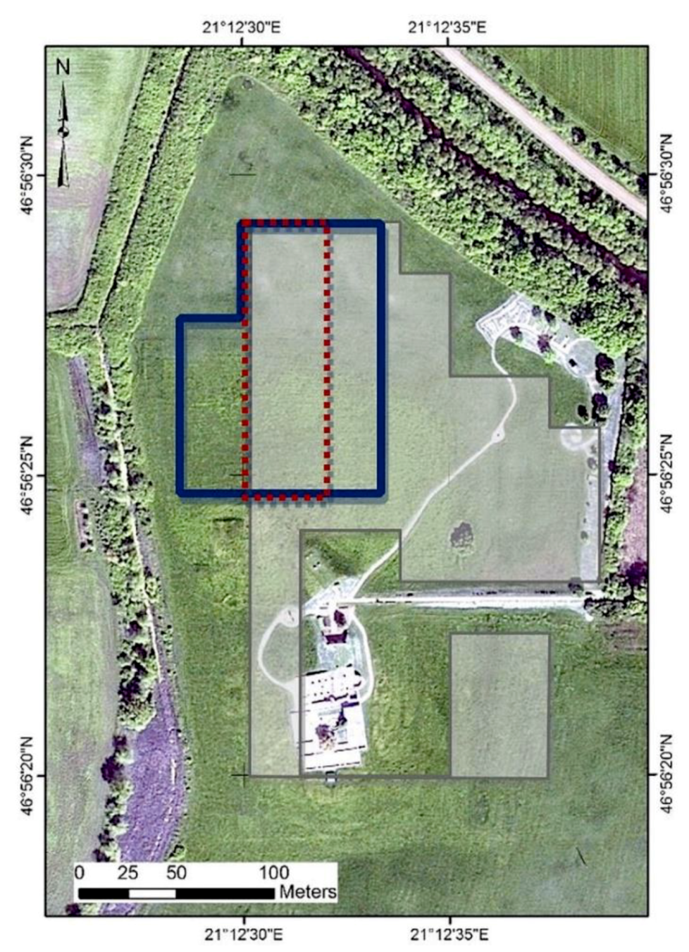
2.1. Case Study Area
2.2. Data Sources
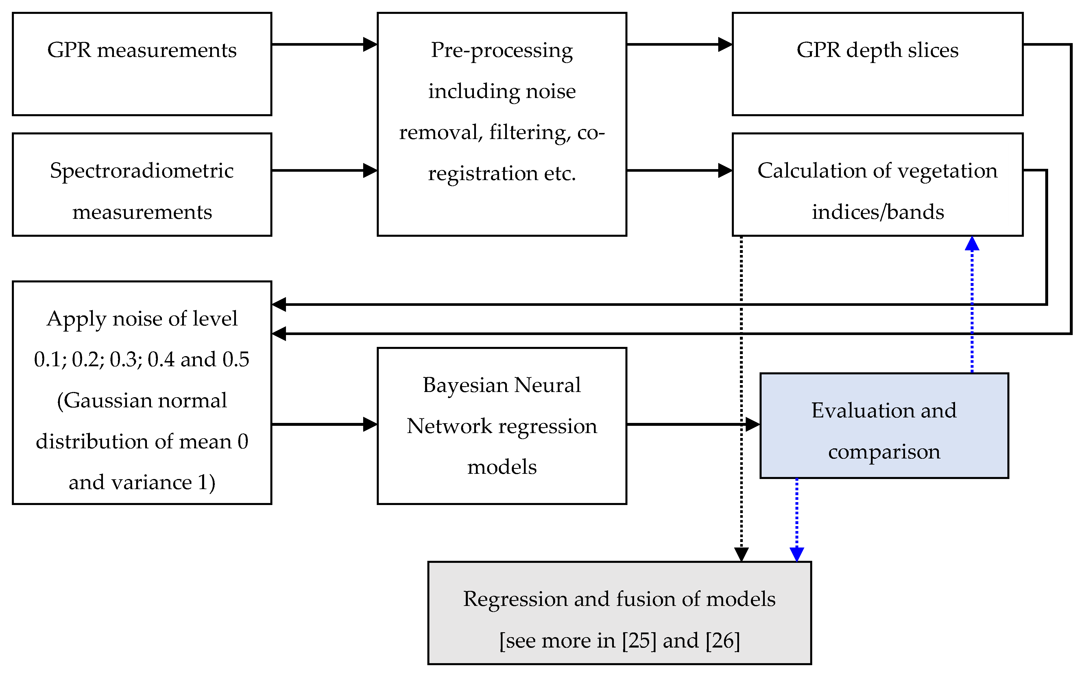
3. Methodology
4. Results
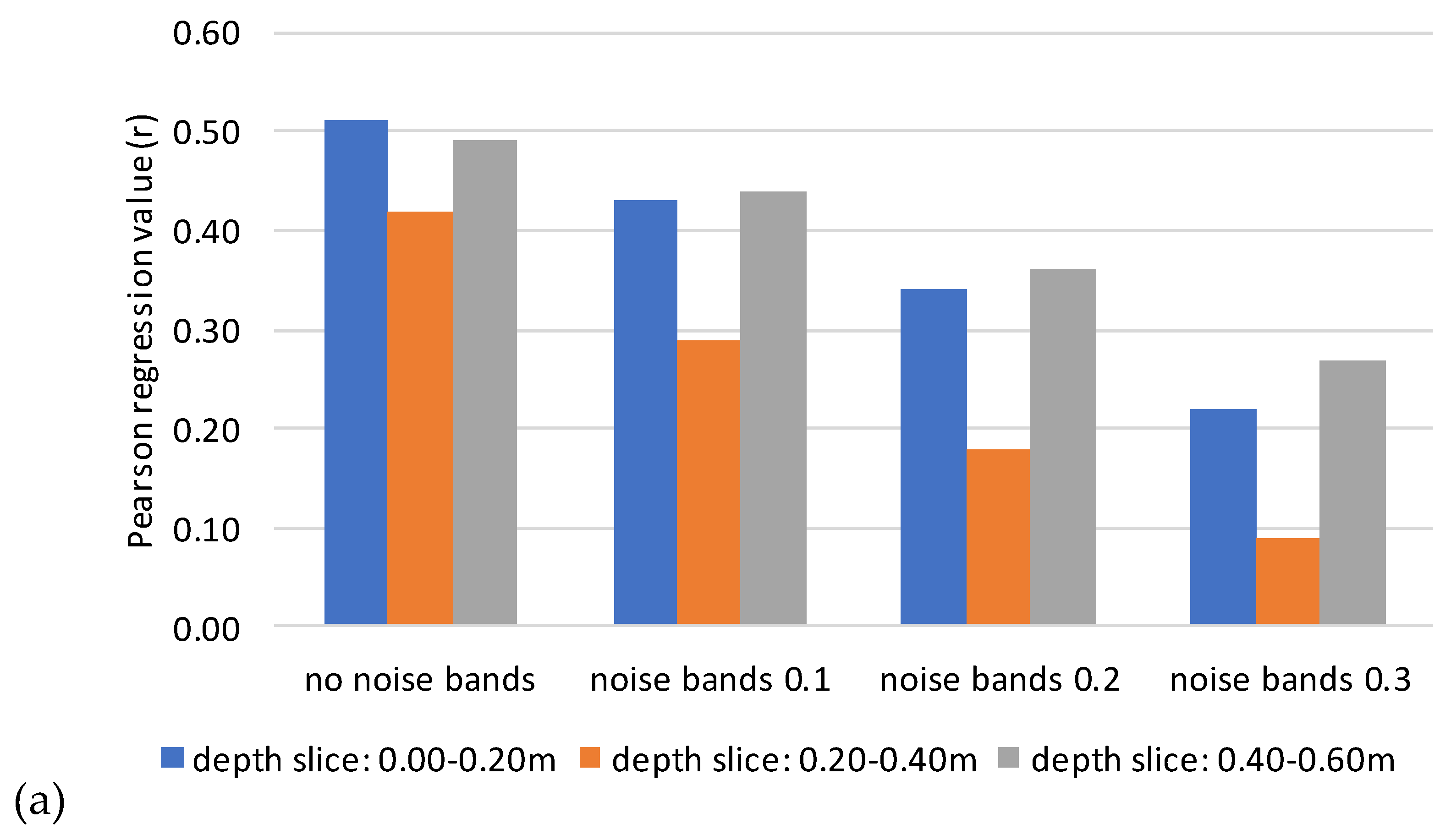
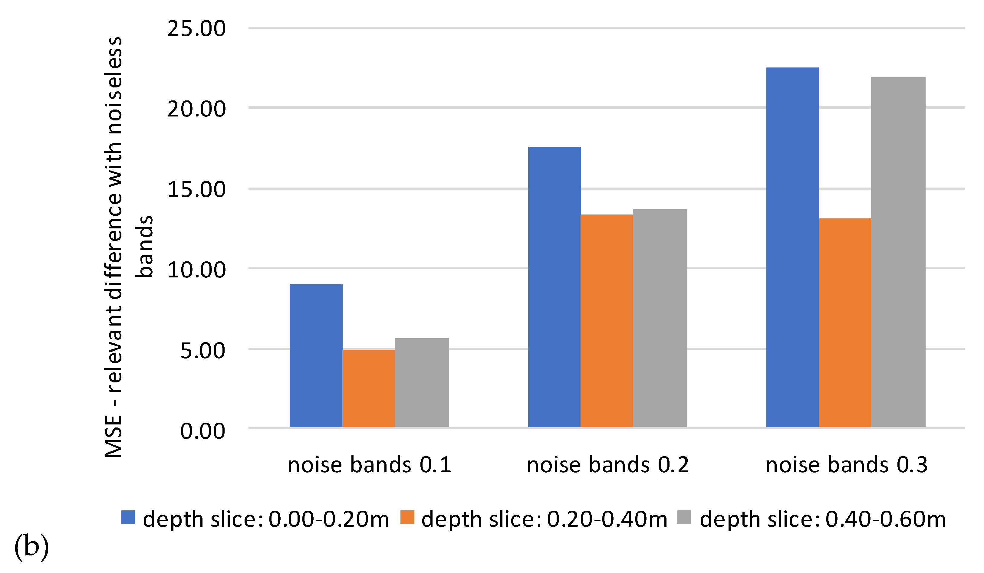
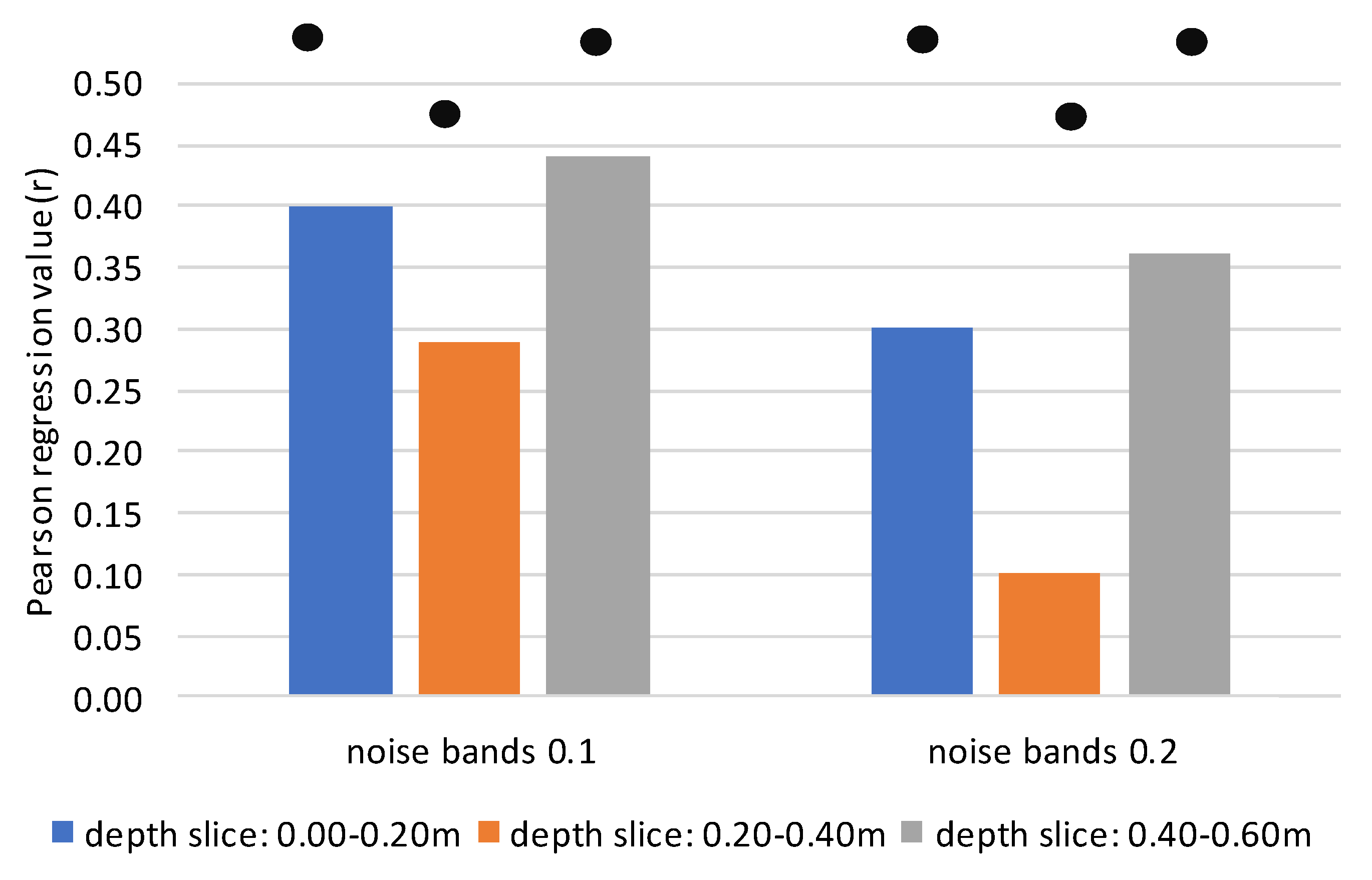
4.1. Random Noise at Spectral Bands
4.2. Random Noise at GPR Depth Slices
4.3. Random Noise at Spectral Bands and GPR Depth Slices
4.4. Random Noise and Vegetation Indices
5. Discussion
- Finding-1: Noise applied either in the optical or the radar datasets decrease the overall correlation fitting performance. However, the noise of levels 0.1 and 0.2 does not dramatically drop the regression value, especially in the case when we used hyperspectral indices in the regression models. This noise can be for instance generated from atmospheric effects or from the sensitivity level of the sensor. Therefore, any potential noise can be minimized through a series of pre-processing steps as, for instance, the radiometric and atmospheric corrections implemented to optical datasets. In addition, external noise can be minimized once the datasets are collected concurrently, or at least when the climate conditions are the same (e.g., no humidity; no rainfall in the previous days). A survey protocol that minimizes potential noise can be of great importance in these cases as it will provide the overall guidelines and framework for the data collection in the field.
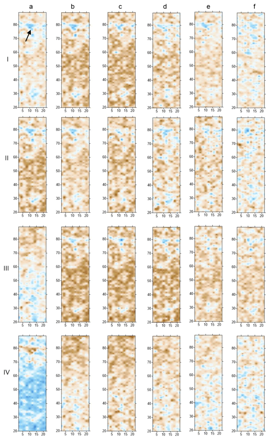
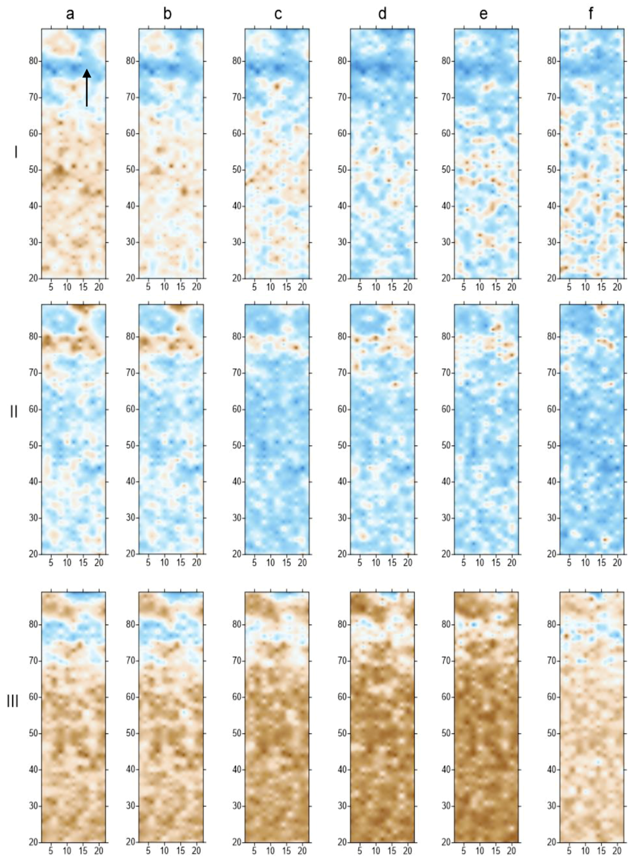
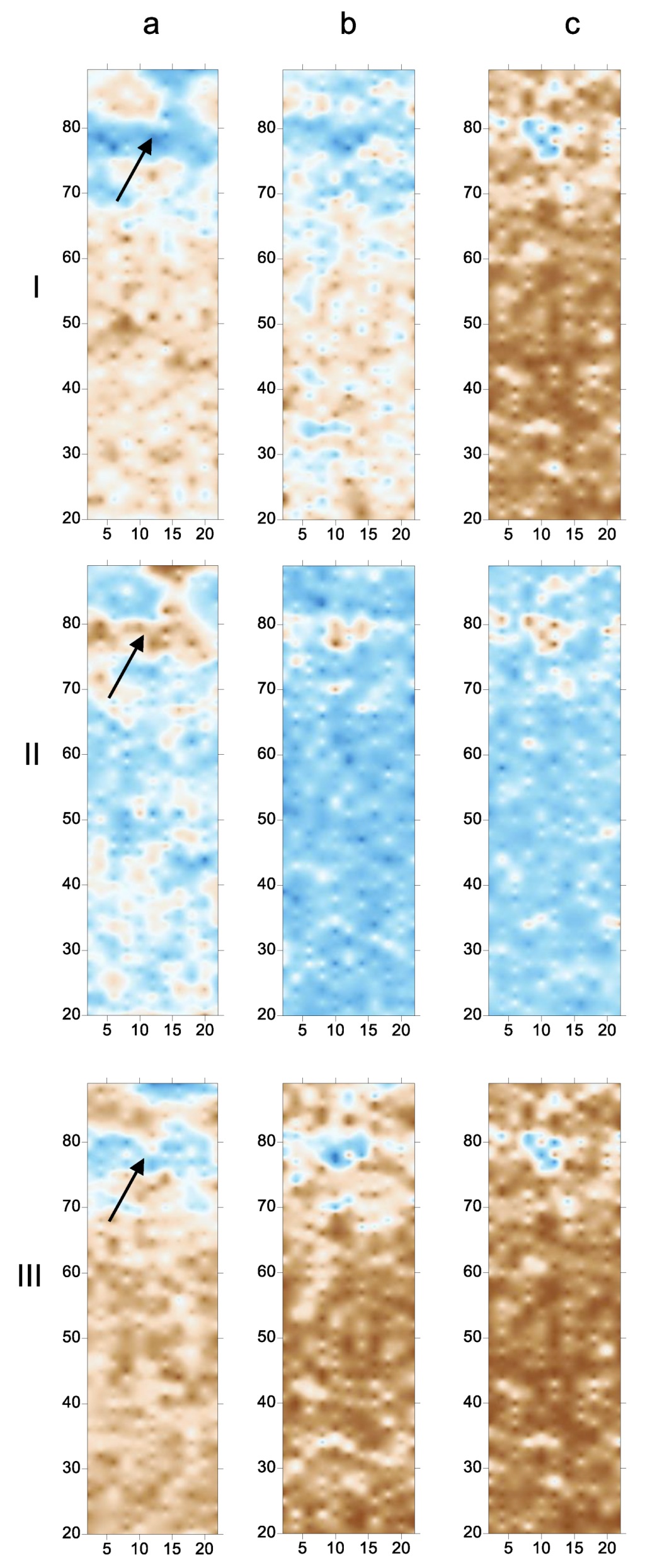
- Finding-2: Anomalies appearing as strong reflectors in the GPR/spectroradiometer measurements, continue to provide an obvious contrast even with noisy datasets. Therefore, the synergistic use of diverse datasets can be implemented for detecting strong anomalies, which are usually identified as priority areas of interest in archaeological surveys. Strong anomalies are expected to be found in areas where the sub-surface target (archaeological remains?) has different properties in contrast to the surrounding soil matrix. The detection or not of such anomalies is also based on the capabilities and characteristics of the remote sensors used in the survey, which are sensitive to only a part of the spectrum.
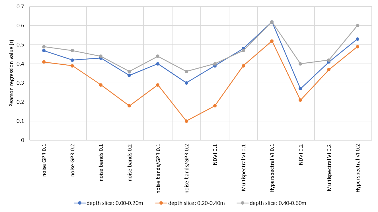
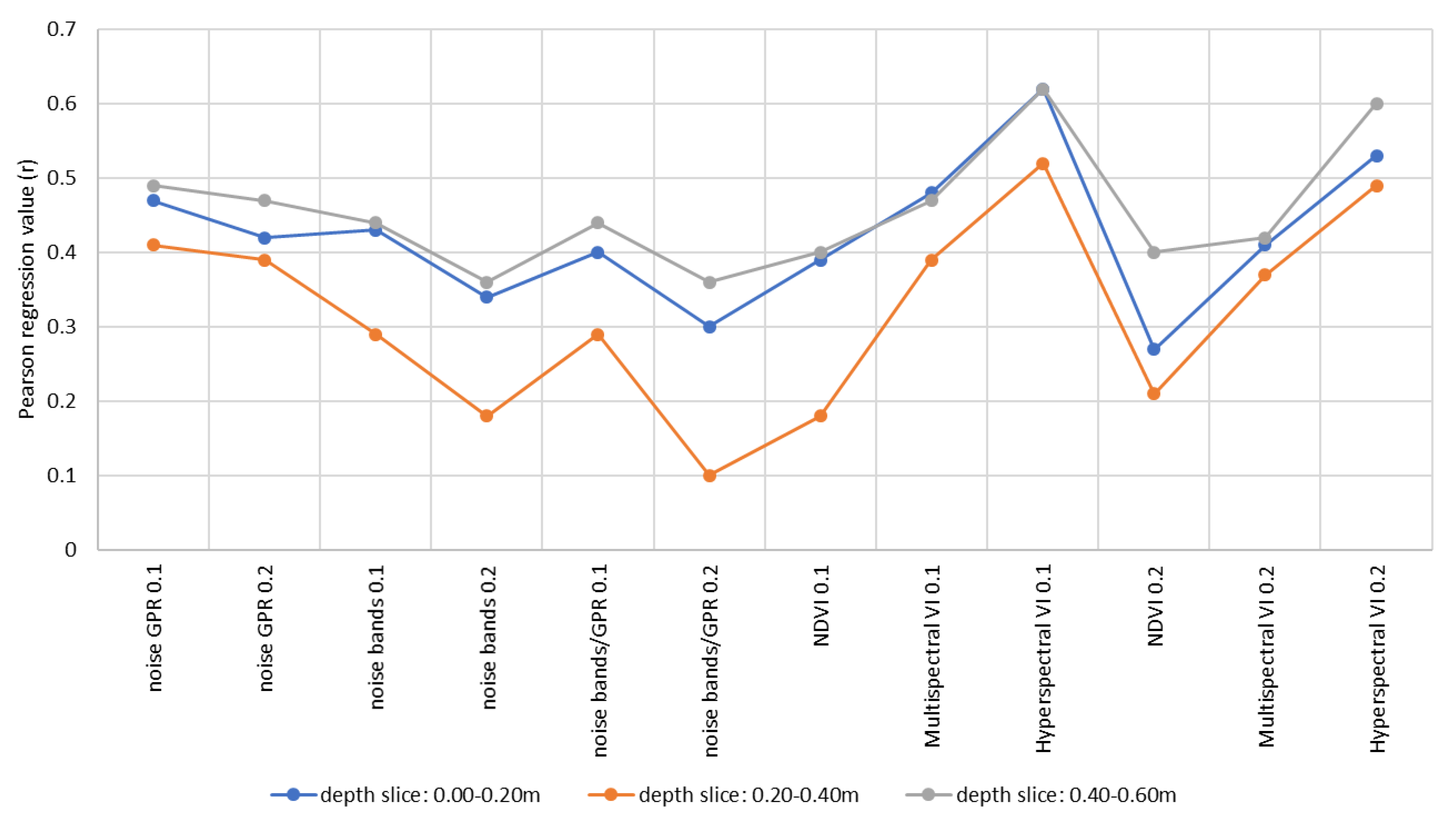
- Finding-3: Vegetation indices provided the best correlation between the optical and GPR datasets. Figure 11 summarizes the overall results regarding the regression values for all different regression combinations between the spectroradiometric and GPR datasets, with an added noise of levels 0.1 and 0.2. The multispectral and hyperspectral indices tend to give the highest regression values r of up to 0.6 while the remaining datasets provided lower regression values (from 0.1 up to 0.5). This observation was compatible with the results found by Agapiou and Sarris in previous studies [25], indicating that processing of the raw datasets (e.g., reflectance values into vegetation indices) can further enhance the contrast of the sub-surface target. While the use of multispectral indices can be generated by most of the earth observation sensors, the use of hyperspectral indices is restricted to a limited number of sensors such as EO-Hyperion 1 (not active), and the Environmental Mapping and Analysis Program (EnMAP).
- Finding-4: Regression fitting beyond the 0.6 meters (not shown in this paper) provided very low correlation coefficient (less than 0.10), allowing us to suggest that any correlation between optical and GPR can be performed only for the upper layers of soil until a depth of approximately 0.6 m. This was once again compatible with the earlier studies of the authors [25]. However, this finding needs to be further investigated with other types of vegetation having different root system characteristics and under different soil properties.
6. Conclusions
Author Contributions
Funding
Acknowledgments
Conflicts of Interest
Appendix A

| No | Vegetation Index | Equation | Reference |
|---|---|---|---|
| 1 | NDVI (Normalized Difference Vegetation Index) | (pNIR − pred)/(pNIR + pred) | [36] |
| 2 | RDVI (Renormalized Difference Vegetation Index) | (pNIR − pred)/(pNIR + pred)1/2 | [37] |
| 3 | IRG (Red Green Ratio Index) | pRed − pgreen | [38] |
| 4 | PVI (Perpendicular Vegetation Index) | (pNIR − α pred − b)/(1 + α2) pNIR,soil = α pred,soil + b | [39] |
| 5 | RVI (Ratio Vegetation Index) | pred/pNIR | [40] |
| 6 | TSAVI (Transformed Soil Adjusted Vegetation Index) | [α(pNIR − α pNIR − b)]/[ (pred + α pNIR −αb + 0.08(1 + α2))] pNIR,soil = α pred,soil + b | [41] |
| 7 | MSAVI (Modified Soil Adjusted Vegetation Index) | [2 pNIR + 1 − [(2 pNIR + 1)2-8(pNIR - pred)]1/2]/2 | [42] |
| 8 | ARVI (Atmospherically Resistant Vegetation Index) | (pNIR – prb)/(pNIR + prb), prb = pred − γ (pblue − pred) | [43] |
| 9 | GEMI (Global Environment Monitoring Index) | n(1 − 0.25n)(pred − 0.125)/(1 − pred) n = [2(pNIR2 − pred2) + 1.5 pNIR + 0.5 pred]/(pNIR + pred + 0.5) | [44] |
| 10 | SARVI (Soil and Atmospherically Resistant Vegetation Index) | (1 + 0.5) (pNIR − prb)/(pNIR + prb + 0.5) prb = pred − γ (pblue − pred) | [42] |
| 11 | OSAVI (Optimized Soil Adjusted Vegetation Index) | (pNIR − pred)/(pNIR + pred + 0.16) | [45] |
| 12 | DVI (Difference Vegetation Index) | pNIR − pred | [46] |
| 13 | SR × NDVI (Simple Ratio x Normalized Difference Vegetation Index | (pNIR2 − pred)/(pNIR + pred2) | [47] |
| No | Vegetation Index | Equation | Reference |
|---|---|---|---|
| 1 | CARI (Chlorophyll Absorption Ratio Index) | p700|α670 + p670 + b|/[p670(α2 + 1)0.5 α = (p700 − p550)/150 b = p550 − 550 α | [48] |
| 2 | GI (Greenness Index) | p554/p677 | [49] |
| 3 | GVI (Greenness Vegetation Index) | (p682 − p553)/(p682 + p553) | [50] |
| 4 | MCARI (Modified Chlorophyll Absorption Ratio Index) | [(P700 − P670) − 0.2(P700 − P550)](P700/P670) | [51] |
| 5 | MCARI2 (Modified Chlorophyll Absorption Ratio Index) | 1.2[2.5(p800 − p670) − 1.3(p800 − p550)] | [52] |
| 6 | mNDVI (Modified Normalized Difference Vegetation Index) | (p800 − p680)/(p800 + p680 − 2 p445) | [53] |
| 7 | SR705 (Simple Ratio, Estimation of chlorophyll content) | p750/p705 | [54] |
| 8 | mNDVI2 (Modified Normalized Difference Vegetation Index) | (p750 − p705)/(p750 + p705 − 2 p445) | [53] |
| 9 | MSAVI (Improved Soil Adjusted Vegetation Index) | [2 p800 + 1 − [(2 p800 + 1)2-8(p800 – p670)]1/2]/2 | [36] |
| 10 | mSR (Modified Simple Ratio) | (p800 − p445)/(p680 − p445) | [53] |
| 11 | mSR2 (Modified Simple Ratio) | (p800 − p445)/(p680 − p445) | [53] |
| 12 | mSR3 (Modified Simple Ratio) | (p800/p670 − 1)/(p800/p670 + 1)0.5 | [55] |
| 13 | MTCI (MERIS Terrestrial Chlorophyll Index) | (p754 − p709)/(p709 − p681) | [56] |
| 14 | mTVI (modified Triangular Vegetation Index) | 1.2[1.2(p800 − p550) − 2.5(p670 − p550)] | [53] |
| 15 | NDVI (Normalized Difference Vegetation Index) | (p800 − p670)/(p800 + p670) | [36] |
| 16 | NDVI2 (Normalized Difference Vegetation Index) | (p750 − p705)/(p750 + p705) | [57] |
| 17 | OSAVI (Optimized Soil Adjusted Vegetation Index) | 1.16(p800 − p670)/(p800 + p670 + 0.16) | [45] |
| 18 | RDVI (Renormalized Difference Vegetation Index) | (p800 − p670)/(p800 + p670)0.5 | [37] |
| 19 | REP(Red-Edge Position) | 700+40[(p670 + p780)/2 – p700]/(p740 – p700) | [58] |
| 20 | SIPI (Structure Insensitive Pigment Index) | (p800 − p450)/(p800 − p650) | [59] |
| 21 | SIPI2 (Structure Insensitive Pigment Index) | (p800 − p440)/(p800 − p680) | [59] |
| 22 | SIPI3(Structure Insensitive Pigment Index) | (p800 − p445)/(p800 − p680) | [60] |
| 23 | SPVI (Spectral polygon vegetation index) | 0.4[3.7(p800 − p670) − 1.2|p530 − p670|] | [61] |
| 24 | SR (Simple Ratio) | p800/p680 | [62] |
| 25 | SR1 (Simple Ratio) | p750/p700 | [63] |
| 26 | SR2 (Simple Ratio) | p752/p690 | [63] |
| 27 | SR3 (Simple Ratio) | p750/p550 | [63] |
| 28 | SR4 (Simple Ratio) | p672/p550 | [64] |
| 29 | TCARI (Transformed Chlorophyll Absorption Ratio Index) | 3[(p700 − p670) − 0.2(p700 − p550)(p700/p670)] | [65] |
| 30 | TSAVI (Transformed Soil Adjusted Vegetation Index) | [α(p875-α p680 –b)]/[ (p680 +α p875 –αb + 0.08(1 + α2))] α = 1.062 b = 0.022 | [45] |
| 31 | TVI (Triangular Vegetation Index) | 0.5[120(p750 − p550) − 200(p670 − p550)] | [66] |
| 32 | VOG (Vogelmann Indices) | p740/p720 | [67] |
| 33 | VOG2 (Vogelmann Indices) | (p734 − p747)/(p715 + p726) | [68] |
| 34 | ARI (Anthocyanin Reflectance Index) | (1/p550) − (1/p700) | [69] |
| 35 | ARI2 (Anthocyanin Reflectance Index 2) | p800(1/p550) − (1/p700) | [69] |
| 36 | BGI (Blue Green Pigment Index) | p450/p550 | [49] |
| 37 | BRI (Blue Red Pigment Index) | p450/p690 | [49] |
| 38 | CRI (Carotenoid Reflectance Index) | (1/p510) − (1/p550) | [70] |
| 39 | RGI (Red/Green Index) | p690/p550 | [49] |
| 40 | CI (Curvature Index) | p675. p690/p2683 | [49] |
| 41 | LIC (Curvature Index) | p440/p690 | [71] |
| 42 | NPCI (Normalized Pigment Chlorophyll index) | (p680 − p430)/(p680 + p430) | [72] |
| 43 | NPQI (Normalized Phaeophytinization Index) | (p415 − p435)/(p415 + p435) | [73] |
| 44 | PRI (Photochemical Reflectance Index) | (p531 − p570)/(p531 + p570) | [74] |
| 45 | PRI2 (Photochemical Reflectance Index) | (p570 − p539)/(p570 + p539) | [75] |
| 46 | PSRI (Plant Senescence Reflectance Index) | (p680 − p500)/p750 | [76] |
| 47 | SR5 (Simple Ratio) | p690/p655 | [49] |
| 48 | SR6(Simple Ratio) | P685/p655 | [49] |
| 49 | VS (Vegetation Stress ratio) | P725/p702 | [77] |
| 50 | MVSR (Modified Vegetation Stress ratio) | P723/p700 | [77] |
| 51 | fWBI (floating Water Band Index) | p900/min p920 − 980 | [78] |
| 52 | WI (Water Index) | p900/p970 | [78] |
| 53 | SG (Sum Green Index) | mean of reflectance across the 500 nm to 600 nm | [38] |
References
- Tapete, D.; Cigna, F. COSMO-SkyMed SAR for Detection and Monitoring of Archaeological and Cultural Heritage Sites. Remote Sens. 2019, 11, 1326. [Google Scholar] [CrossRef]
- Stewart, C.; Oren, E.D.; Cohen-Sasson, E. Satellite Remote Sensing Analysis of the Qasrawet Archaeological Site in North Sinai. Remote Sens. 2018, 10, 1090. [Google Scholar] [CrossRef]
- Simyrdanis, K.; Papadopoulos, N.; Cantoro, G. Shallow Off-Shore Archaeological Prospection with 3-D Electrical Resistivity Tomography: The Case of Olous (Modern Elounda), Greece. Remote Sens. 2016, 8, 897. [Google Scholar] [CrossRef]
- Schultz, J.J.; Martin, M.M. Controlled GPR grave research: Comparison of reflection profiles between 500 and 250 MHz antenna. Forensic Sci. Int. 2011, 209, 64–69. [Google Scholar] [CrossRef] [PubMed]
- Hansen, D.J.; Pringle, K.J.; Goodwin, J. GPR and bulk ground resistivity surveys in graveyards: Locating unmarked burials in contrasting soil types. Forensic Sci. Int. 2014, 237, e14–e29. [Google Scholar] [CrossRef]
- Harrison, M.; Donnelly, L.J. Locating concealed homicide victims: Developing the role of geoforensics. In Criminal and Environmental Soil Forensics; Ritz, K., Dawson, L., Miller, D., Eds.; Springer: Dordrecht, The Netherland, 2009; pp. 197–219. [Google Scholar]
- De Coster, A.; Pérez Medina, J.L.; Nottebaere, M.; Alkhalifeh, K.; Neyt, X.; Vanderdonckt, J.; Lambot, S. Towards an improvement of GPR-based detection of pipes and leaks in water distribution networks. J. Appl. Geophys. 2019, 162, 138–151. [Google Scholar] [CrossRef]
- Park, B.; Kim, J.; Lee, J.; Kang, M.-S.; An, Y.-K. Underground Object Classification for Urban Roads Using Instantaneous Phase Analysis of Ground-Penetrating Radar (GPR) Data. Remote Sens. 2018, 10, 1417. [Google Scholar] [CrossRef]
- Ayala-Cabrera, D.; Izquierdo, J.; Pérez-García, R.; Herrera, M. Location of buried plastic pipes using multi-agent support based on GPR images. J. Appl. Geophys. 2011, 75, 679–686. [Google Scholar] [CrossRef]
- Bechtel, T.; Truskavetsky, S.; Pochanin, G.; Capineri, L.; Sherstyuk, A.; Viatkin, K.; Byndych, T.; Ruban, V.; Varyanitza-Roschupkina, L.; Orlenko, O.; et al. Characterization of Electromagnetic Properties of In Situ Soils for the Design of Landmine Detection Sensors: Application in Donbass, Ukraine. Remote Sens. 2019, 11, 1232. [Google Scholar] [CrossRef]
- Núñez-Nieto, X.; Solla, M.; Gómez-Pérez, P.; Lorenzo, H. GPR Signal Characterization for Automated Landmine and UXO Detection Based on Machine Learning Techniques. Remote Sens. 2014, 6, 9729–9748. [Google Scholar] [CrossRef]
- Borie, C.; Parcero-Oubiña, C.; Kwon, Y.; Salazar, D.; Flores, C.; Olguín, L.; Andrade, P. Beyond Site Detection: The Role of Satellite Remote Sensing in Analysing Archaeological Problems. A Case Study in Lithic Resource Procurement in the Atacama Desert, Northern Chile. Remote Sens. 2019, 11, 869. [Google Scholar] [CrossRef]
- Fuldain González, J.J.; Varón Hernández, F.R. NDVI Identification and Survey of a Roman Road in the Northern Spanish Province of Álava. Remote Sens. 2019, 11, 725. [Google Scholar] [CrossRef]
- Rayne, L.; Donoghue, D. A Remote Sensing Approach for Mapping the Development of Ancient Water Management in the Near East. Remote Sens. 2018, 10, 2042. [Google Scholar] [CrossRef]
- Kalaycı, T.; Sarris, A. Multi-Sensor Geomagnetic Prospection: A Case Study from Neolithic Thessaly, Greece. Remote Sens. 2016, 8, 966. [Google Scholar] [CrossRef]
- Cozzolino, M.; Longo, F.; Pizzano, N.; Rizzo, M.L.; Voza, O.; Amato, V. A Multidisciplinary Approach to the Study of the Temple of Athena in Poseidonia-Paestum (Southern Italy): New Geomorphological, Geophysical and Archaeological Data. Geosciences 2019, 9, 324. [Google Scholar] [CrossRef]
- Kalayci, T.; Simon, F.-X.; Sarris, A. A Manifold Approach for the Investigation of Early and Middle Neolithic Settlements in Thessaly, Greece. Geosciences 2017, 7, 79. [Google Scholar] [CrossRef]
- Caspari, G.; Sadykov, T.; Blochin, J.; Buess, M.; Nieberle, M.; Balz, T. Integrating Remote Sensing and Geophysics for Exploring Early Nomadic Funerary Architecture in the “Siberian Valley of the Kings”. Sensors 2019, 19, 3074. [Google Scholar] [CrossRef] [PubMed]
- Alexakis, A.; Sarris, A.; Astaras, T.; Albanakis, K. Integrated GIS, remote sensing and geomorphologic approaches for the reconstruction of the landscape habitation of Thessaly during the Neolithic period. J. Archaeol. Sci. 2011, 38, 89–100. [Google Scholar] [CrossRef]
- Traviglia, A.; Cottica, D. Remote sensing applications and archaeological research in the Northern Lagoon of Venice: The case of the lost settlement of Constanciacus. J. Archaeol. Sci. 2011, 38, 2040–2050. [Google Scholar] [CrossRef]
- Yu, L.; Zhang, Y.; Nie, Y.; Zhang, W.; Gao, H.; Bai, X.; Liu, F.; Hategekimana, Y.; Zhu, J. Improved detection of archaeological features using multi-source data in geographically diverse capital city sites. J. Cult. Herit. 2018, 33, 145–158. [Google Scholar] [CrossRef]
- Opitz, R.; Herrmann, J. Recent Trends and Long-standing Problems in Archaeological Remote Sensing. J. Comput. Appl. Archaeol. 2018, 1, 19–41. [Google Scholar] [CrossRef]
- Leisz, S.J. An overview of the application of remote sensing to archaeology during the twentieth century. In Mapping Archaeological Landscapes from Space; Springer: New York, NY, USA, 2013; pp. 11–19. [Google Scholar]
- Kvamme, K.L. Geophysical correlation: global versus local perspectives. Archaeol. Prospect. 2018, 25, 111–120. [Google Scholar] [CrossRef]
- Agapiou, A.; Sarris, A. Beyond GIS Layering: Challenging the (Re) use and Fusion of Archaeological Prospection Data Based on Bayesian Neural Networks (BNN). Remote Sens. 2018, 10, 1762. [Google Scholar] [CrossRef]
- Agapiou, A.; Lysandrou, V.; Sarris, A.; Papadopoulos, N.; Hadjimitsis, D.G. Fusion of Satellite Multispectral Images Based on Ground-Penetrating Radar (GPR) Data for the Investigation of Buried Concealed Archaeological Remains. Geosciences 2017, 7, 40. [Google Scholar] [CrossRef]
- Sarris, A.; Papadopoulos, N.; Agapiou, A.; Salvi, M.C.; Hadjimitsis, D.G.; Parkinson, A.; Yerkes, R.W.; Gyucha, A.; Duffy, R.P. Integration of geophysical surveys, ground hyperspectral measurements, aerial and satellite imagery for archaeological prospection of prehistoric sites: The case study of Vésztő-Mágor Tell, Hungary. J. Archaeol. Sci. 2013, 40, 1454–1470. [Google Scholar] [CrossRef]
- Gyucha, A.; Yerkes, W.R.; Parkinson, A.W.; Sarris, A.; Papadopoulos, N.; Duffy, R.P.; Salisbury, B.R. Settlement Nucleation in the Neolithic: A Preliminary Report of the Körös Regional Archaeological Project’s Investigations at Szeghalom-Kovácshalom and Vésztő-Mágor. In Neolithic and Copper Age between the Carpathians and the Aegean Sea: Chronologies and Technologies from the 6th to the 4th Millennium BCE; Hansen, S., Raczky, P., Anders, A., Reingruber, A., Eds.; International Workshop Budapest: Bonn, Germany, 2012; pp. 129–142. [Google Scholar]
- Hegedűs, K. Vésztő-Mágori-domb. In Magyarország Régészeti Topográfiája VI; Ecsedy, I., Kovács, L., Maráz, B., Torma, I., Eds.; Békés Megye Régészeti Topográfiája: A Szeghalmi Járás; Akadémiai Kiadó: Budapest, Hungary, 1982; pp. 184–185. [Google Scholar]
- Hegedűs, K.; Makkay, J. Vésztő-Mágor: A Settlement of the Tisza Culture. In The Late Neolithic of the Tisza Region: A Survey of Recent Excavations and Their Findings; Tálas, L., Raczky, P., Eds.; Szolnok County Museums: Szolnok, Hungary, 1987; pp. 85–104. [Google Scholar]
- Makkay, J. Vésztő–Mágor. In Ásatás a Szülőföldön; Békés Megyei Múzeumok Igazgatósága: Békéscsaba, Hungary, 2004. [Google Scholar]
- Parkinson, W.A. Tribal Boundaries: Stylistic Variability and Social Boundary Maintenance during the Transition to the Copper Age on the Great Hungarian Plain. J. Anthropol. Archaeol. 2006, 25, 33–58. [Google Scholar] [CrossRef]
- Juhász, I. A Csolt nemzetség monostora. In A középkori Dél-Alföld és Szer; Kollár, T., Ed.; Csongrád Megyei Levéltár: Szeged, Hungary, 2000; pp. 281–304. [Google Scholar]
- Neal, R.M. Bayesian Learning for Neural Networks; Springer Science & Business Media: New York, NY, USA, 2012; p. 118. [Google Scholar]
- Luo, L.; Wang, X.; Guo, H.; Lasaponara, R.; Zong, X.; Masini, N.; Wang, G.; Shi, P.; Khatteli, H.; Chen, F.; et al. Airborne and spaceborne remote sensing for archaeological and cultural heritage applications: A review of the century (1907–2017). Remote Sens. Environ. 2019, 232, 111280. [Google Scholar] [CrossRef]
- Rouse, J.W.; Haas, R.H.; Schell, J.A.; Deering, D.W.; Harlan, J.C. Monitoring the Vernal Advancements and Retrogradation (Greenwave Effect) of Nature Vegetation; NASA/GSFC Final Report; NASA: Greenbelt, MD, USA, 1974.
- Roujean, J.L.; Breon, F.M. Estimating PAR absorbed by vegetation from bidirectional reflectance measurements. Remote Sens. Environ. 1995, 51, 375–384. [Google Scholar] [CrossRef]
- Gamon, J.A.; Surfus, J.S. Assessing leaf pigment content and activity with a reflectometer. New Phytol. 1999, 143, 105–117. [Google Scholar] [CrossRef]
- Richardson, A.J.; Wiegand, C.L. Distinguishing vegetation from soil background information. Photogramm. Eng. Remote Sens. 1977, 43, 15–41. [Google Scholar]
- Pearson, R.L.; Miller, L.D. Remote Mapping of Standing Crop Biomass and Estimation of the Productivity of the Short Grass Prairie, Pawnee National Grasslands, Colorado. In Proceedings of the 8th International Symposium on Remote Sensing of the Environment, Ann Arbor, MI, USA, 2–6 October 1972; pp. 1357–1381. [Google Scholar]
- Baret, F.; Guyot, G. Potentials and limits of vegetation indices for LAI and APAR assessment. Remote Sens. Environ. 1991, 35, 161–173. [Google Scholar] [CrossRef]
- Qi, J.; Chehbouni, A.; Huete, A.R.; Kerr, Y.H.; Sorooshian, S. A modified soil adjusted vegetation index. Remote Sens. Environ. 1994, 48, 119–126. [Google Scholar] [CrossRef]
- Kaufman, Y.J.; Tanré, D. Atmospherically resistant vegetation index (ARVI) for EOS-MODIS. IEEE Trans. Geosci. Remote Sens. 1992, 30, 261–270. [Google Scholar] [CrossRef]
- Pinty, B.; Verstraete, M.M. GEMI: A non-linear index to monitor global vegetation from satellites. Plant Ecol. 1992, 101, 15–20. [Google Scholar] [CrossRef]
- Rondeaux, G.; Steven, M.; Baret, F. Optimization of soil-adjusted vegetation indices. Remote Sens. Environ. 1996, 55, 95–107. [Google Scholar] [CrossRef]
- Tucker, C.J. Red and photographic infrared linear combinations for monitoring vegetation. Remote Sens. Environ. 1979, 8, 127–150. [Google Scholar] [CrossRef]
- Gong, P.; Pu, R.; Biging, G.S.; Larrieu, M.R. Estimation of forest leaf area index using vegetation indices derived from Hyperion hyperspectral data. IEEE Trans. Geosci. Remote Sens. 2003, 41, 1355–1362. [Google Scholar] [CrossRef]
- Kim, M.S.; Daughtry, C.S.T.; Chappelle, E.W.; McMurtrey, J.E., III; Walthall, C.L. The Use of High Spectral Resolution Bands for Estimating Absorbed Photosynthetically Active Radiation (APAR). In Proceedings of the 6th Symposium on Physical Measurements and Signatures in Remote Sensing, Val D’Isere France, 17–21 January 1994. [Google Scholar]
- Zarco-Tejada, P.J.; Berjón, A.; López-Lozano, R.; Miller, J.R.; Martín, P.; Cachorro, V.; González, M.R.; de Frutos, A. Assessing vineyard condition with hyperspectral indices: Leaf and canopy reflectance simulation in a row-structured discontinuous canopy. Remote Sens. Environ. 2005, 99, 271–287. [Google Scholar] [CrossRef]
- Gandia, S.; Fernández, G.; García, J.C.; Moreno, J. Retrieval of Vegetation Biophysical Variables from CHRIS/PROBA Data in the SPARC Campaing. In Proceedings of the 4th ESA CHRIS PROBAWorkshop, Frascati, Italy, 28–30 April 2004; pp. 40–48. [Google Scholar]
- Daughtry, C.S.T.; Walthall, C.L.; Kim, M.S.; de Colstoun, E.B.; McMurtrey, J.E. Estimating corn leaf chlorophyll concentration from leaf and canopy reflectance. Remote Sens. Environ. 2000, 74, 229–239. [Google Scholar] [CrossRef]
- Haboudane, D.; Miller, J.R.; Pattey, E.; Zarco-Tejada, P.J.; Strachan, I. Hyperspectral vegetation indices and novel algorithms for predicting green LAI of crop canopies: Modeling and validation in the context of precision agriculture. Remote Sens. Environ. 2004, 90, 337–352. [Google Scholar] [CrossRef]
- Sims, D.A.; Gamon, J.A. Relationships between leaf pigment content and spectral reflectance across a wide range of species, leaf structures and developmental stages. Remote Sens. Environ. 2002, 81, 337–354. [Google Scholar] [CrossRef]
- Castro-Esau, K.L.; Sánchez-Azofeifa, G.A.; Rivard, B. Comparison of spectral indices obtained using multiple spectroradiometers. Remote Sens. Environ. 2006, 103, 276–288. [Google Scholar] [CrossRef]
- Chen, J.; Cihlar, J. Retrieving leaf area index of boreal conifer forests using Landsat Thematic Mapper. Remote Sens. Environ. 1996, 55, 153–162. [Google Scholar] [CrossRef]
- Dash, J.; Curran, P.J. The MERIS terrestrial chlorophyll index. Int. J. Remote Sens. 2004, 25, 5403–5413. [Google Scholar] [CrossRef]
- Gitelson, A.; Merzlyak, M.N. Quantitative estimation of chlorophyll-a using reflectance spectra: Experiments with autumn chestnut and maple leaves. J. Photochem. Photobiol. B Biol. 1994, 22, 247–252. [Google Scholar] [CrossRef]
- Guyot, G.; Baret, F.; Major, D.J. High spectral resolution: Determination of spectral shifts between the red and near infrared. Int. Arch. Photogramm. Remote Sens. Spat. Inf. Sci. 1988, 11, 750–760. [Google Scholar]
- Peñuelas, J.; Filella, I.; Lloret, P.; Munoz, F.; Vilajeliu, M. Reflectance assessment of mite effects on apple trees. Int. J. Remote Sens. 1995, 16, 2727–2733. [Google Scholar] [CrossRef]
- Penuelas, J.; Baret, F.; Filella, I. Semi-empirical indices to assess carotenoids/chlorophyll-a ratio from leaf spectral reflectance. Photosynthetica 1995, 31, 221–230. [Google Scholar]
- Vincini, M.; Frazzi, E.; D’Alessio, P. Angular Dependence of Maize and Sugar Beet Vis from Directional CHRIS/PROBA Data. In Proceedings of the 4th ESA CHRIS PROBA Workshop, Frascati, Italy, 19–21 September 2006; pp. 19–21. [Google Scholar]
- Jordan, C.F. Derivation of leaf area index from quality of light on the forest floor. Ecology 1969, 50, 663–666. [Google Scholar] [CrossRef]
- Gitelson, A.A.; Merzlyak, M.N. Remote estimation of chlorophyll content in higher plant leaves. Int. J. Remote Sens. 1997, 18, 2691–2697. [Google Scholar] [CrossRef]
- Datt, B. Remote sensing of chlorophyll a, chlorophyll b, chlorophyll a+b, and total carotenoid content in eucalyptus leaves. Remote Sens. Environ. 1998, 66, 111–121. [Google Scholar] [CrossRef]
- Haboudane, D.; Miller, J.R.; Tremblay, N.; Zarco-Tejada, P.J.; Dextraze, L. Integrated narrow-band vegetation indices for prediction of crop chlorophyll content for application to precision agriculture. Remote Sens. Environ. 2002, 81, 416–426. [Google Scholar] [CrossRef]
- Broge, N.H.; Leblanc, E. Comparing prediction power and stability of broadband and hyperspectral vegetation indices for estimation of green leaf area index and canopy chlorophyll density. Remote Sens. Environ. 2001, 76, 156–172. [Google Scholar] [CrossRef]
- Vogelmann, J.E.; Rock, B.N.; Moss, D.M. Red edge spectral measurements from sugar maple leaves. Int. J. Remote Sens. 1993, 14, 1563–1575. [Google Scholar] [CrossRef]
- Zarco-Tejada, P.J.; Pushnik, J.C.; Dobrowski, S.; Ustin, S.L. Steady-state chlorophyll a fluorescence detection from canopy derivative reflectance and double-peak red-edge effects. Remote Sens. Environ. 2003, 84, 283–294. [Google Scholar] [CrossRef]
- Gitelson, A.A.; Merzlyak, M.N.; Chivkunova, O.B. Optical properties and nondestructive estimation of anthocyanin content in plant leaves. Photochem. Photobiol. 2001, 74, 38–45. [Google Scholar] [CrossRef]
- Gitelson, A.A.; Zur, Y.; Chivkunova, O.B.; Merzlyak, M.N. Assessing carotenoid content in plant leaves with reflectance spectroscopy. Photochem. Photobiol. 2002, 75, 272–281. [Google Scholar] [CrossRef]
- Lichtenthaler, H.K.; Lang, M.; Sowinska, M.; Heisel, F.; Miehe, J.A. Detection of vegetation stress via a new high resolution fluorescence imaging system. J. Plant Physiol. 1996, 148, 599–612. [Google Scholar] [CrossRef]
- Peñuelas, J.; Gamon, J.A.; Fredeen, A.L.; Merino, J.; Field, C.B. Reflectance indices associated with physiological changes in nitrogen- and water-limited sunflower leaves. Remote Sens. Environ. 1994, 48, 135–146. [Google Scholar] [CrossRef]
- Barnes, J.D.; Balaguer, L.; Manrique, E.; Elvira, S.; Davison, A.W. A reappraisal of the use of DMSO for the extraction and determination of chlorophylls a and b in lichens and higher plants. Environ. Exp. Bot. 1992, 32, 85–100. [Google Scholar] [CrossRef]
- Gamon, J.A.; Serrano, L.; Surfus, J.S. The photochemical reflectance index: An optical indicator of photosynthetic radiation use efficiency across species, functional types, and nutrient levels. Oecologia 1997, 112, 492–501. [Google Scholar] [CrossRef] [PubMed]
- Filella, I.; Amaro, T.; Araus, J.L.; Peñuelas, J. Relationship between photosynthetic radiation-use efficiency of barley canopies and the photochemical reflectance index (PRI). Physiol. Plant. 1996, 96, 211–216. [Google Scholar] [CrossRef]
- Merzlyak, M.N.; Gitelson, A.A.; Chivkunova, O.B.; Rakitin, V.Y. Nondestructive optical detection of pigment changes during leaf senescence and fruit ripening. Physiol. Plant. 1999, 106, 135–141. [Google Scholar] [CrossRef]
- White, D.C.; Williams, M.; Barr, S.L. Detecting sub-surface soil disturbance using hyperspectral first derivative band rations of associated vegetation stress. Int. Arch. Photogramm. Remote Sens. Spat. Inf. Sci. 2008, 27, 243–248. [Google Scholar]
- Peñuelas, J.; Filella, I.; Biel, C.; Serrano, L.; Savé, R. The reflectance at the 950–970 nm region as an indicator of plant water status. Int. J. Remote Sens. 1993, 14, 1887–1905. [Google Scholar] [CrossRef]


© 2019 by the authors. Licensee MDPI, Basel, Switzerland. This article is an open access article distributed under the terms and conditions of the Creative Commons Attribution (CC BY) license (http://creativecommons.org/licenses/by/4.0/).
Share and Cite
Agapiou, A.; Sarris, A. Working with Gaussian Random Noise for Multi-Sensor Archaeological Prospection: Fusion of Ground Penetrating Radar Depth Slices and Ground Spectral Signatures from 0.00 m to 0.60 m below Ground Surface. Remote Sens. 2019, 11, 1895. https://doi.org/10.3390/rs11161895
Agapiou A, Sarris A. Working with Gaussian Random Noise for Multi-Sensor Archaeological Prospection: Fusion of Ground Penetrating Radar Depth Slices and Ground Spectral Signatures from 0.00 m to 0.60 m below Ground Surface. Remote Sensing. 2019; 11(16):1895. https://doi.org/10.3390/rs11161895
Chicago/Turabian StyleAgapiou, Athos, and Apostolos Sarris. 2019. "Working with Gaussian Random Noise for Multi-Sensor Archaeological Prospection: Fusion of Ground Penetrating Radar Depth Slices and Ground Spectral Signatures from 0.00 m to 0.60 m below Ground Surface" Remote Sensing 11, no. 16: 1895. https://doi.org/10.3390/rs11161895
APA StyleAgapiou, A., & Sarris, A. (2019). Working with Gaussian Random Noise for Multi-Sensor Archaeological Prospection: Fusion of Ground Penetrating Radar Depth Slices and Ground Spectral Signatures from 0.00 m to 0.60 m below Ground Surface. Remote Sensing, 11(16), 1895. https://doi.org/10.3390/rs11161895