1. Introduction
Terrestrial remote sensing technologies, such as terrestrial laser scanning (TLS) and structure from motion (SfM) photogrammetry have been increasingly used to characterize and monitor rock slope hazards [
1,
2,
3,
4], and other geomorphic processes [
5,
6,
7,
8,
9]. They are used to monitor processes at repeat intervals on the order of days to months or years, nevertheless wide spread use as fixed or permanent installation systems has yet to be achieved. At present, Ground-based Interferometric synthetic-aperture radar (GB-InSAR) is widely used for continuous near-real time monitoring of displacements for landslides [
10,
11], open pit mine walls [
12], and rock slopes [
13], as it can obtain deformation measurements at the sub-millimeter level and is not affected by weather conditions [
14]. For some monitoring applications, however, the use of TLS or SfM may be a feasible alternative to radar monitoring as the system cost can be lower, higher ground resolution can be achieved, volumes can be measured, and 3D displacements can be extracted.
With increasing amounts of available data storage, cloud computing, automation, and high-speed connectivity, monitoring geomorphic or hazard processes at a higher frequency with fixed TLS or SFM system is becoming more viable. Terrestrial laser scanning has been used to study slope processes at a high temporal rate (30 min repeat intervals), for the near-real time monitoring of rock slope pre-failure deformation [
15], and to study the degradation of a coastal slope in high temporal detail [
16]. Monitoring at a high frequency has been beneficial to better understand the acceleration behavior prior to a rockfall and to capture short deformation periods [
15]. It also produces a more accurate Magnitude-Frequency (M-F) relationship as compared to measuring at longer time intervals [
16,
17].
Monitoring rock slopes with a fixed array of cameras using photogrammetric techniques to build 3D models can also be a viable alternative to monitoring with TLS for a variety of monitoring applications. A fixed array of cameras has several potential advantages including: an array of cameras that are well positioned can better capture the morphology of the slope than a single TLS station; the use of cameras can be a low-cost alternative to TLS systems; the design of the system (e.g., number of cameras and camera specifications) is fit for purpose and scalable in terms of slope pixel size and level of detectable change; the point clouds have embedded color; and time lapse monitoring facilitates more frequent monitoring compared to repeat site visits.
The first known use of a photogrammetric system for landslide monitoring was by [
18], where a system of two low resolution cameras were used to monitor landslide displacements. The system was meant to provide supplementary data at the site and not a replacement for other monitoring equipment. Preliminary performance tests and quality assessments with a fixed system of cameras were conducted by [
19] for civil engineering applications using a system of five standalone units 8 Megapixel cameras. The use of fixed photogrammetric systems has also extended to the study of continuous geomorphic processes conducted over 15 second time intervals over a period of a day [
20]. Camera calibration procedures for precise change detection were also tested at a rock slope by [
21]. These studies highlight the potential for using fixed array of cameras for monitoring a variety of processes and changes at a wide spectrum at time scales.
In this study, we contribute to this field of research by presenting a new application of an array of cameras to the study of rock slope hazard by long-term monitoring on a daily basis, the development of an automated method for processing data including automation of vegetation removal and point cloud registration with scale adjustment, development of a method that does not require the use of ground control points, and an optimized workflow for high resolution and high precision change detection. We also provide a comparison of the developed technique with a method using ground control points. Furthermore, the study also investigates whether such a system can be a viable alternative for the study of rockfall pre-failure deformation and magnitude frequency relationships. This generally requires the detection of deformation on the cm range [
22,
23,
24,
25].
2. Study Site
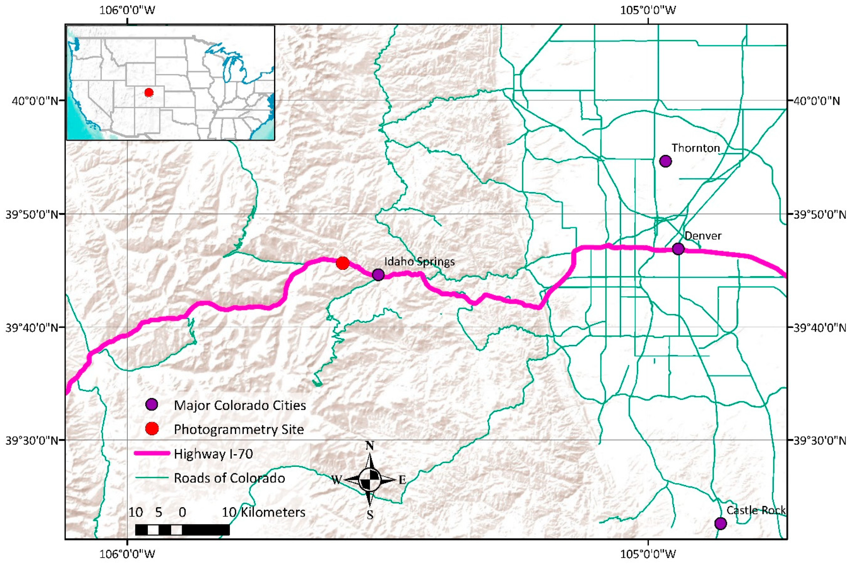
This study is part of a research collaboration with the Colorado Department of Transportation (CDOT), where several rock slope hazard sites are being studied with terrestrial remote monitoring methods. The study area includes slopes along Interstate I70 west from Denver (
Figure 1). The study site chosen for the development and implementation of the time lapse camera system is located 50 km west of Denver and 10 km west of Idaho Springs, within the front range of the Rocky Mountains (
Figure 1).
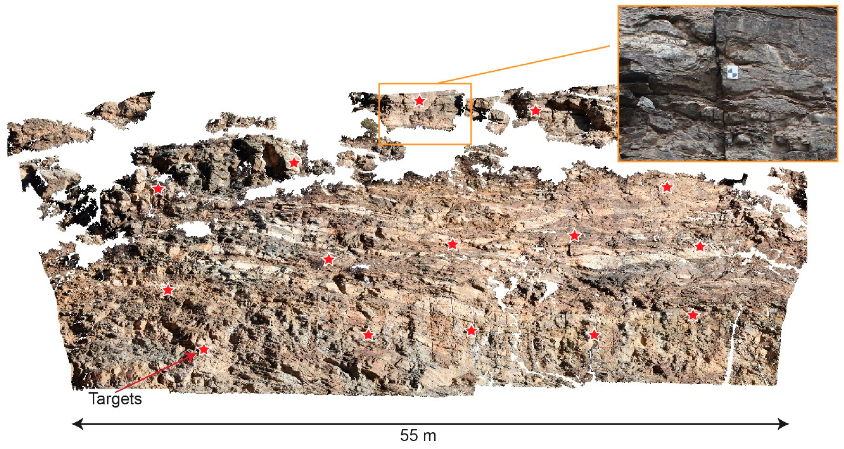
The study area is located within the front range of the Colorado Rocky Mountains. The rocks at the site are Precambrian in age and are part of a gneissic formation composed of interlayered units of biotite gneisses, granite gneiss, and microcline-gneiss [
27]. The study site itself consists of jointed biotite gneiss. The biotite gneiss consists of interlayers of plagioclase-biotite gneiss and sillimanitic biotite-quartz gneiss and is well foliated. The gneissic layering can be identified in the site photograph in
Figure 2. The gneiss is folded along a northeast trending axes, and contains a minimum of two or more joint sets [
28]. The joint system formed during the Larimide Orogeny and the most prominent joints are oriented longitudinal to the folding axis (on average N19W), with cross joints striking east to northeast [
28]. The combination of steep canyons, jointed rock, and seasonal freeze thaw cycles makes this region particularly prone to rockfall hazard.
3. System Design
In general, the design of a camera system is unique to the study site of interest and the requirements to monitor a given phenomenon. Several design variables need to be considered and optimized on a per site basis, including the following:
The distance of the camera network to the target;
The number and locations of the cameras;
The camera resolution and lens configuration;
The available budget;
The size of the monitored area;
Required data resolution and accuracy;
Required monitoring interval;
Sophistication of time lapse controller and associated equipment;
Site access constraints;
Environmental constraints.
Some site characteristics and phenomena may not be suitable for camera monitoring. An example could be a large site requiring high resolution or small ground pixel size. This would require a large network of high resolution cameras. More suitable configurations could include monitoring large displacements over a large area at lower resolution or monitoring small displacements at a high resolution over a smaller area.
The following subsections outline the required components of the camera system and the design considerations for rockfall monitoring using a time lapse system.
3.1. System Components
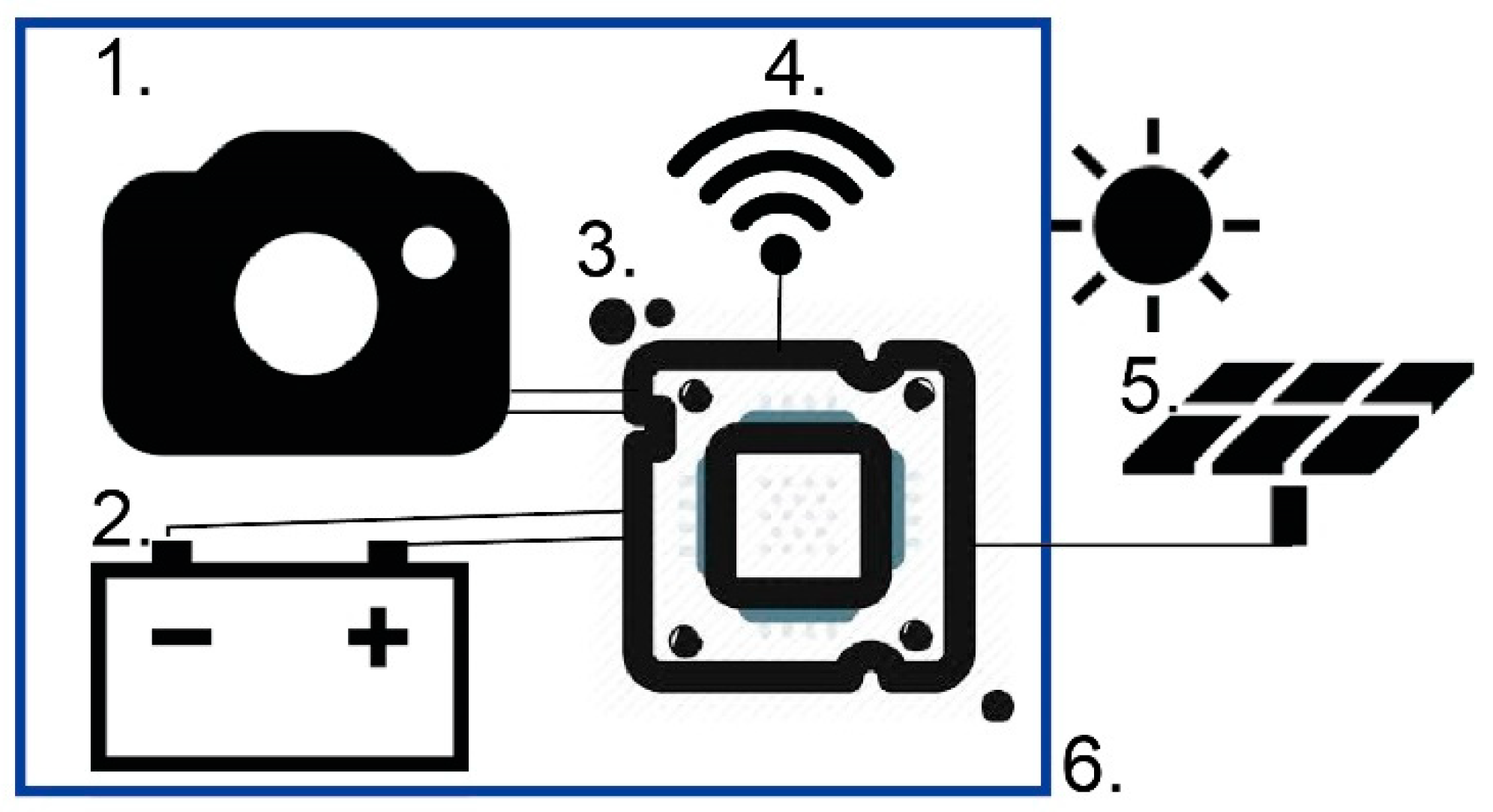
For indefinite data collection, the system needs to operate autonomously, have its own power supply, be protected from weather, and operate reliably in various weather conditions. The system used for this study consists of a camera and lens, a solar panel, an internal battery pack, a microcomputer controller, a wireless internet connection, and a weatherproof and tamperproof protective housing (
Figure 3).
Such systems can be designed using low cost computers such as Raspberry Pis and custom designed protective housing [
19]. For this study, to ensure reliable long term operation and camera protection, a commercial system housing and microcomputer Cyclapse [
29] was used (
Figure 4, inset A).
3.2. Camera and Lens
The choice of camera depends on the target resolution required to be able to detect the process of interest and the site geometry. There are many low-cost camera options, which may be suitable in some applications, including small sensor systems, action cameras, cell phone cameras, and network video cameras. For rockfall monitoring, high quality photos and high resolution cameras are necessary to be able to detect fragmental rockfall volumes and small precursor changes occurring on the slope. There is a correlation between higher end and higher resolution cameras and 3D model accuracy [
30]. For this reason, Canon 5DSR cameras with 50-megapixel resolution were used for this study.
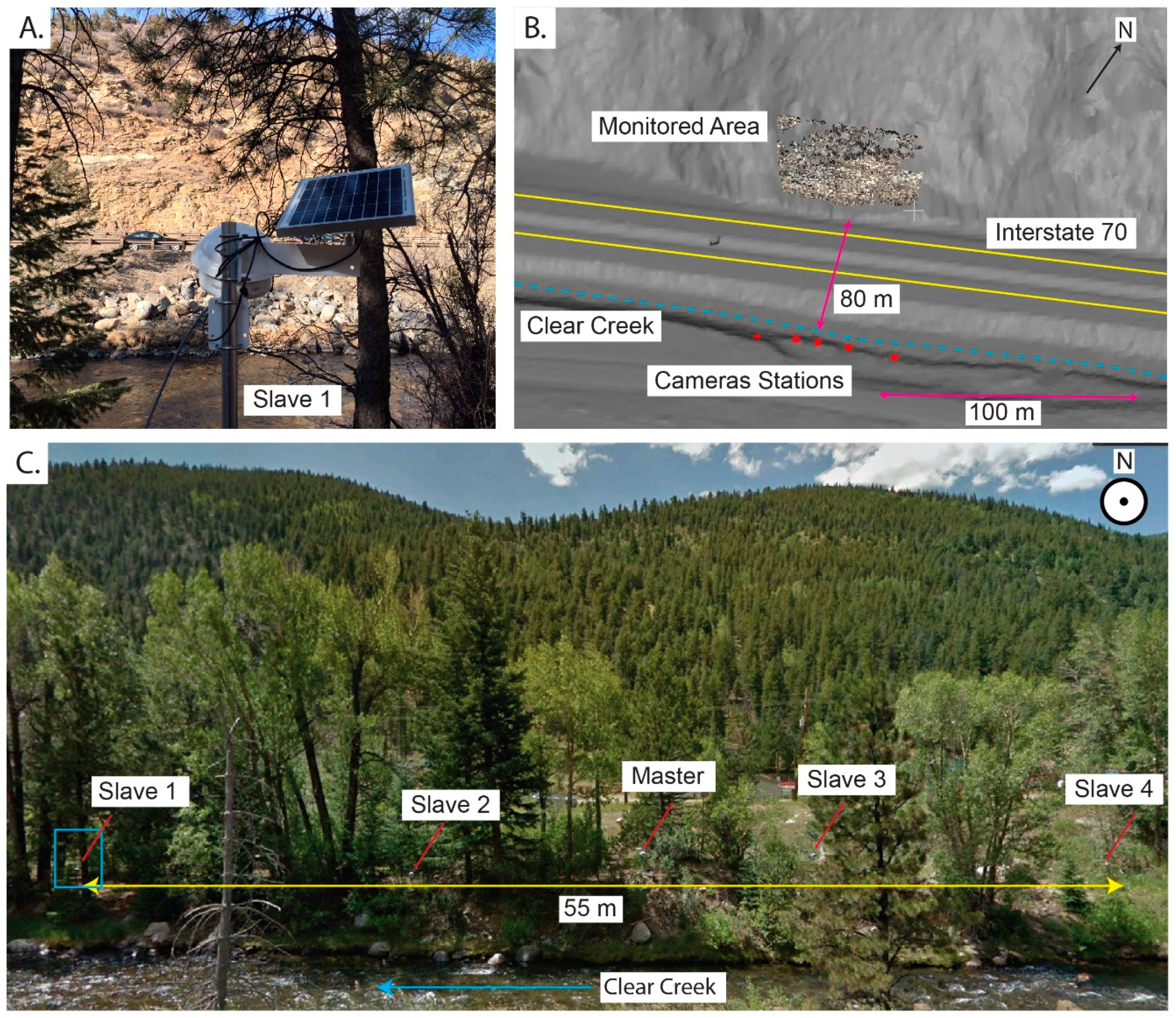
The locations of the cameras were constrained to the opposite side of Clear Creek at an 80 m average distance to the slope. Canon EF 85 mm prime lenses were selected to maximize coverage of the scene.
3.3. Camera System Setup and Geometry
The camera system was designed with five individual camera stations, installed 80 m from the slope on the opposing river bank of Clear Creek (
Figure 4, Inset B and C). The system was designed to trigger photos from a single control station (master controller). The master controller sends a signal to the other camera stations (slave controllers) via connected cables, allowing near simultaneous photo collection. The system can also trigger photos from each individual camera station based on their internal clocks.
Each camera station was between 10 and 15 m apart with a distance to base ratio ranging between 1:5 and 1:8. The camera stations were installed on the river bank and were approximately parallel to the target rock slope. The placement of the cameras allowed for a central photo having 50% overlap with the photos from the intermediate stations, and outer station photos having 100% overlap with the intermediate stations.
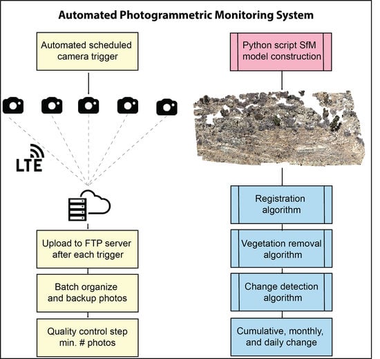
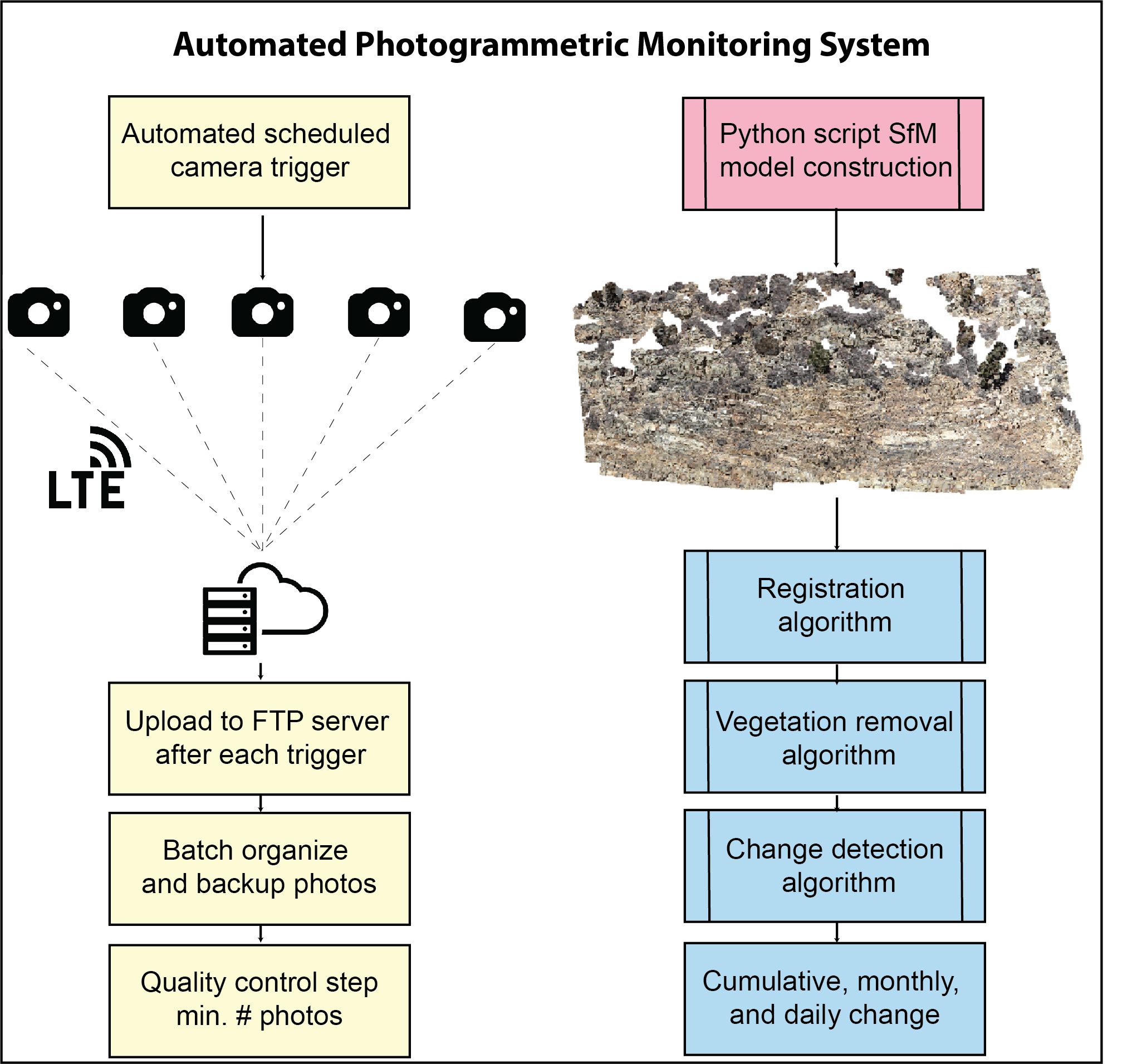
4. Automated Workflow
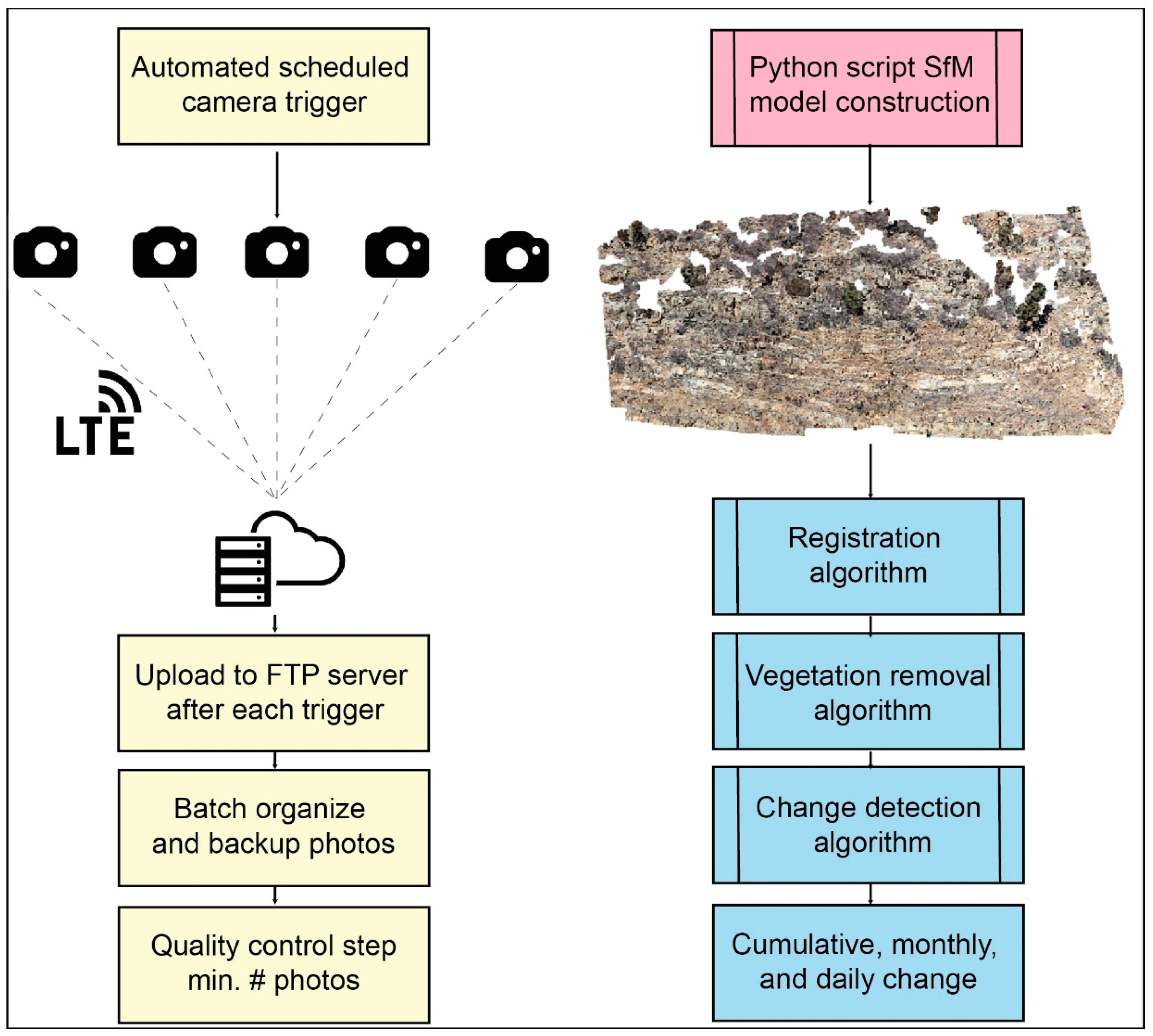
The automated data processing workflow consists of three components: (1) Schedule picture and upload of data; (2) SfM construction of 3D models; and (3) a registration and change detection pipeline (
Figure 5). The workflow is designed for use to monitor an area without ground control points. The workflow requires some initial manual processing steps prior to initiating automation. This includes setting the schedule of pictures, providing a scaled and referenced SfM model as a reference for registration, and providing a classified point cloud with vegetation for vegetation removal. A detailed description of the three steps can be found in the following subsections.
4.1. Automated Camera Control
Each camera station consists of a programmable microcomputer and USB LTE modem that controls when pictures are taken, manages power consumption, and transfers data to a server. Pictures are taken at a set time every day and the time is synchronized using the network connection. After each transfer, a batch script on the processing computer fetches, organizes and backs-up the photos. If a minimum number of photos were not collected (i.e., due to system errors), the SfM model construction is not initiated, preventing poor model constructions.
4.2. SFM Model Construction
Agisoft Photoscan v.1.4.5. [
31] was used for construction of the 3D photogrammetric models via an automated script using Python v.3.7.3 [
32]. The script is initiated after photos are uploaded to the FTP server.
In Photoscan, sparse point cloud construction was conducted using the highest accuracy settings, disabling generic or reference pre-selection and adaptive fitting, and not limiting the number of tie points detected per image to maximize tie point detection. An upper limit of 500,000 matching keypoints was used.
Tie points with outlier reprojection errors (>2 standard deviations) were filtered and removed iteratively. One iteration consisted of a reduced filtered reprojection error, removal of points above the filtered values, and the optimization of camera parameters and/or camera locations. The iterative procedure stopped after a set number of iterations or once the remaining number of tie points reached the lower threshold of 100,000 tie points.
Dense point clouds were constructed using a medium density setting, typically generating point clouds with 7,000,000 points corresponding to a ground point spacing of 0.02 m. Tests at ultra-high density produced models of greater than 70,000,000 points, which led to computational issues in later stages of processing. The medium density setting was therefore deemed appropriate for automatic processing purposes.
4.3. Automated Registration with Scale
The proposed method of registration without ground control requires that real-world scale and orientation (translation, rotation, scale) be determined and applied to the 3D photogrammetric models. Real world scale is modeled using a single terrestrial laser scan of the site. A photogrammetric model is manually aligned and scaled to the reference TLS point cloud. This photogrammetric model becomes the reference model for registration for all subsequent models.
Development of automated registration algorithms has mainly been for TLS-derived point clouds (e.g., [
33,
34,
35,
36]) within the fields of robotics, computer vision, and photogrammetry. Applications incorporating automated alignment with scale difference are still in early development [
37,
38,
39]. In this work, an automated registration algorithm with scale was developed in C++, which relies in part on the similarity of successive point clouds in a fixed position multi-camera setup. The steps used in the algorithm are outlined in
Figure 6. The algorithm is based on the open-source point cloud library (PCL) [
36] and estimates scale using a four-step process where the estimation gradually becomes more refined: (1) Initial rough estimation based on ratio of resolution; (2) fast point feature histogram matching and ratio of principal eigenvalues; (3) rigid alignment and singular value decomposition (SVD) scale estimation; and (4) refinement with an iterative corresponding point (ICP) algorithm with scale.
4.3.1. Ratio of Resolution
To get an initial rough estimation of scale, the similarity between subsequent point clouds is taken advantage of, and scale is estimated based on the ratio of resolutions of the reference alignment model and the aligned model. Since successive photogrammetric models are created using identical parameters, the resolutions of the models vary minimally, and any minor deviations depend primarily on the quality of the photos.
4.3.2. Fast Point Feature Histogram Matching and Ratio of Principle Eigenvalues
In the second step of the algorithm, the point clouds are down-sampled by a factor of ten times the cloud resolution using a voxel down-sampling method to decrease processing time. For each of the down sampled points, fast point feature histograms are calculated using the PCL [
36]. The algorithm calculates multidimensional histograms of values for each point encoding the geometric characteristics surrounding the point. The histograms are then used to obtain correspondences between point clouds. A random sample consensus (RANSAC) based correspondence rejecter implemented in PCL [
36] is used to remove poor correspondence matches. Point clouds are then created for the data and reference cloud consisting of the remaining matches. Eigenvalues are calculated for each point in the correspondence point clouds. The ratio of each of the three principal components from each cloud is calculated, and the average of the three ratios is used as the scale factor for this step.
4.3.3. Rigid Alignment and SVD Scale Estimation
At this stage, a rigid transformation and rotation is applied. This is done by finding correspondence between the reference and data subsampled point clouds using the calculated featured histograms. The correspondences are filtered using RANSAC and the best transformation is obtained. The transformation estimation using singular value decomposition with scale estimation from PCL is implemented to refine the rotation, translation, and scale.
4.3.4. Iterative Registration
The final step is to refine the registration using an iterative corresponding point algorithm with scale adjustment. Within this algorithm, correspondences are estimated between points (not features) using a normal shooting method, poor correspondences are rejected using a median rejecter, and the transformation is estimated using singular value decomposition with scale using PCL functions [
36]. These steps are repeated until a preset stopping criterion is met.
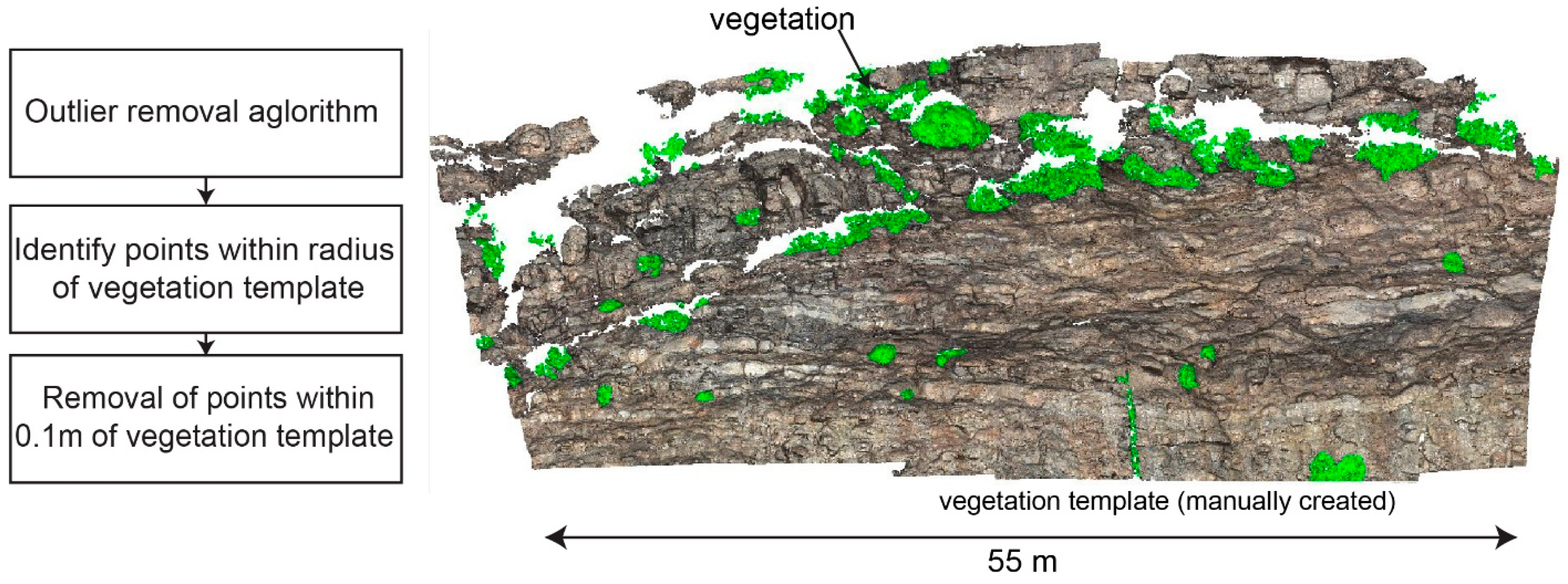
4.4. Vegetation Filtering
Following registration, vegetation is filtered from the aligned point cloud. To automate the vegetation removal, a template of vegetation points is first manually made from a series of 3D models of the site. The template consists of the subset of the total model points consisting of vegetation. The vegetation removal algorithm first removes outliers using a statistical outlier removal algorithm. The algorithm performs a statistical analysis on each point’s neighborhood distances and removes points that are outside 2 standard deviations of neighborhood distance. The nearest neighbors within a 0.1 m radius of each vegetation point are then found and removed from the point cloud.
Figure 7 illustrates an example of the vegetation template and workflow for this step.
4.5. Change Detection Algorithm
A change detection algorithm based on slope-dependent normals was implemented. Normals are calculated and the comparison direction is set based on the reference model normal direction. The difference is calculated along the normal to a subset of closest points in the data model. The mean location along the vector is then used as the raw distance. The raw distances are then filtered using a nearest neighbor averaging filter. This change detection algorithm was originally implemented by [
15].
Prior to implementation of the automated algorithm, an optimum normal radius was determined by cycling through a series of normal radius distances and finding which radius minimized the error between two models, as in [
16].
Within the automated workflow, change is calculated cumulatively from the reference model, change in the prior 30 days, and change on a daily basis. The daily change data are used to identify rockfall events and calculate their volumes. The cumulative change data are used to identify and plot pre-failure deformations prior to rockfall events.
5. Experimental Methods
5.1. Target-Based Models
As a check and to assess the accuracy of the proposed monitoring approach without ground control points, targets were installed on the slope. Fifteen 15 cm diameter targets were installed, spread equally throughout the scene (see
Figure 2). The target locations were surveyed with a total station from the opposing river bank of Clear Creek with an accuracy of 3 mm.
A separate manual method was used to construct a SfM model using the surveyed ground control in the scene. Each target was manually identified in Photoscan and the surveyed coordinates were assigned to the targets. The same model construction settings and procedure was used for the ground control-based construction as for the previously described approach without ground control.
5.2. Time Lapse Data Collection
Time lapse data was collected on a daily basis since 19 March 2018. Pictures were taken using aperture priority with an F8 aperture settings and an ISO setting of 100. Each camera in the system was set to take photos at 12:00 pm and 12:30 pm daily.
For two days, 7 and 8 July 2018, photos were collected every 30 min from 9:00 to 16:00. The purpose of the test was to see if we could improve the overall accuracy and precision of the model by taking repeated photographs and whether improved model quality could be observed in areas typically affected by low sun exposure.
5.3. Pre-Calibration and Intrinsic Camera Parameters
To optimize SfM model construction, various pre-calibration approaches for the determination of intrinsic camera parameters were tested and applied to all of the time series data collected. Models were constructed using fixed pre-calibration (intrinsic parameters fixed), using pre-calibration and allowing adjustment of the intrinsic parameters during bundle adjustment, and using no pre-calibration and solving for the intrinsic parameters during bundle adjustment. Models were also constructed using separate pre-calibration parameters for each camera station and using one set of pre-calibration parameters for all cameras.
To determine pre-calibration parameters, Agisoft Lens [
31] was first used with the built-in checkerboard. This however, did not provide representative intrinsic camera parameters due to difficulty in simulating the field focus and camera settings in a lab setting. The intrinsic camera parameters were then determined using self-calibration with bundle adjustment. Pictures of the field site with the installed targets were taken for each camera while installed in the protective housing. This ensured that the calibration procedure accounted for the additional outer layer of glass on the protective housing. The intrinsic camera parameters were then solved within Agisoft Photoscan [
31]. Ideally, this self-calibration procedure should be done in a separate calibration field to provide better accuracy intrinsic camera parameters and because the proposed procedure does not rely on targets being installed at the field site. For this study, the assumption is that using the targets installed at the field site closely approximates a calibration field.
As a test, pre-calibration parameters were also extracted from the solved intrinsic parameters from a model constructed without pre-calibration. These parameters were then used as a set of artificial pre-calibration parameters and applied to all models in the time series.
6. Results
6.1. Spatial Assessment of Accuracy
To assess the effects of using a method without ground control and the effects of different pre-calibration settings on spatial accuracy, the TLS scan was used as a reference for change comparison. The distribution of differences in comparing the TLS to the SfM models was used to assess the model accuracy. This was done by analyzing the statistics of the differences and assessing the spatial distributions of differences qualitatively.
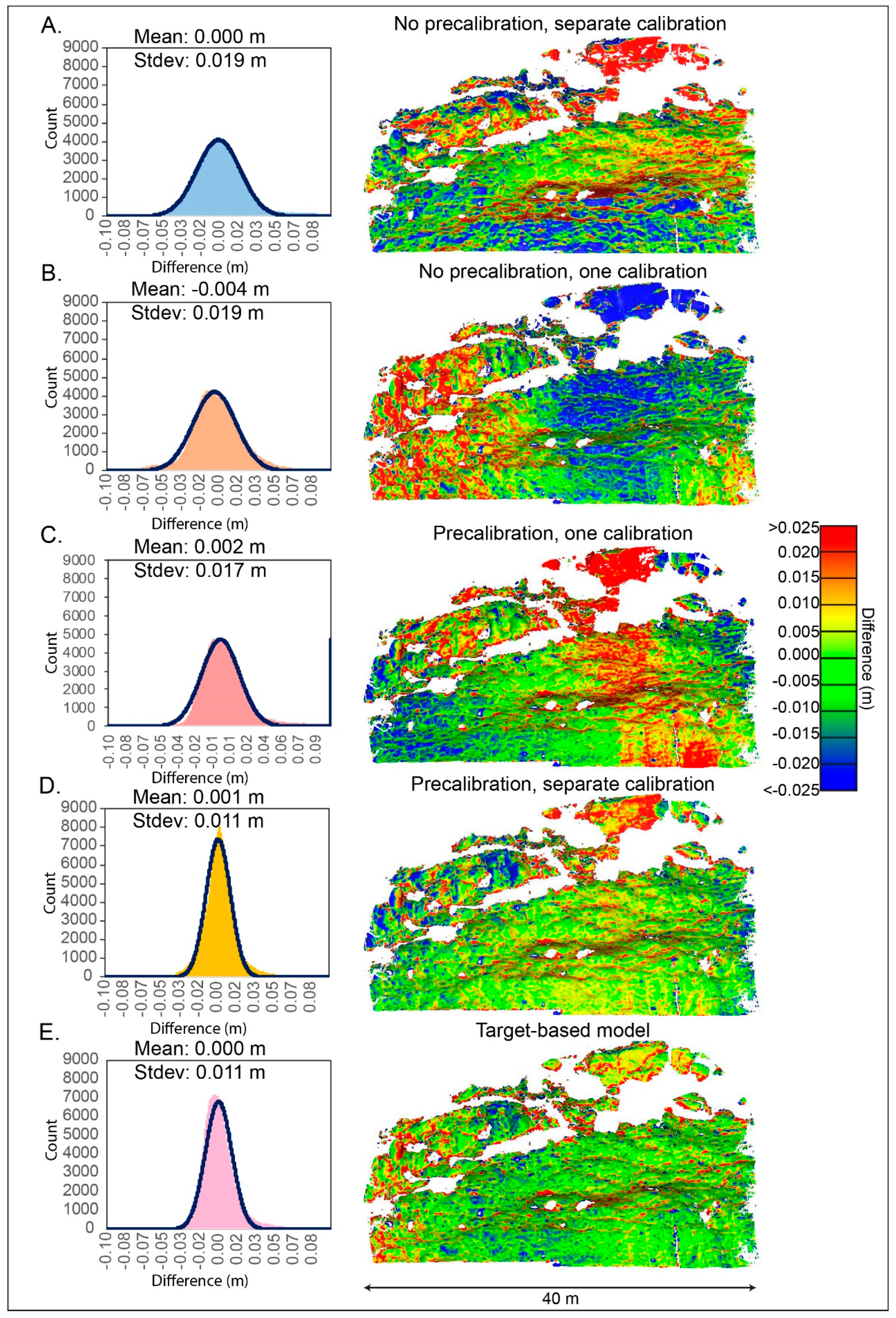
Figure 8 shows the comparison between TLS and five different SfM model constructions: (1) No pre-calibration with separate calibration parameters for each camera; (2) no pre-calibration with one calibration group for all cameras: (3) pre-calibration with one calibration group for all camera; (4) pre-calibration with separate calibration parameters for each camera; (5) a model constructed using ground control. The figure shows the resulting differences as histograms and spatially distributed over the comparison area for qualitative assessment of accuracy.
The target-based model (
Figure 8, Inset E) produced, on average, 0.01 m error on each target compared to the surveyed coordinates. This error is also reflected in the comparison of the target model with the TLS reference, which resulted in a standard deviation of differences of 0.011 m. Qualitatively, the spatial distribution of residuals is random and uniformly distributed, indicating a good agreement with the TLS reference scan.
The pre-calibrated model constructed with separate calibration parameters for each camera (
Figure 8, Inset D) is comparable to the target-based model with a standard deviation of 0.011 m. However, qualitatively the accuracy differs. The spatial distribution of residuals is uniform in the central part of the model, however deviates slightly around the periphery, indicating a slight distortion in the model.
Both model constructions without using pre-calibration are of lesser accuracy. The model constructed with separate calibration groups (
Figure 8, Inset A) produced a standard deviation of 0.019 m. The model differences are uniformly distributed in the central parts of the model, but significant systematic errors are visible in the upper and lower parts of the model.
The models constructed with the same calibration parameters for all cameras (
Figure 8, Inset B and C) produced standard deviations of 0.017 m and 0.019 m, respectively, for the pre-calibrated and non-pre-calibrated cases. Compared to the separated calibration group constructions, the differences appear with more distortion and appear as a characteristic ‘bowl’ effect.
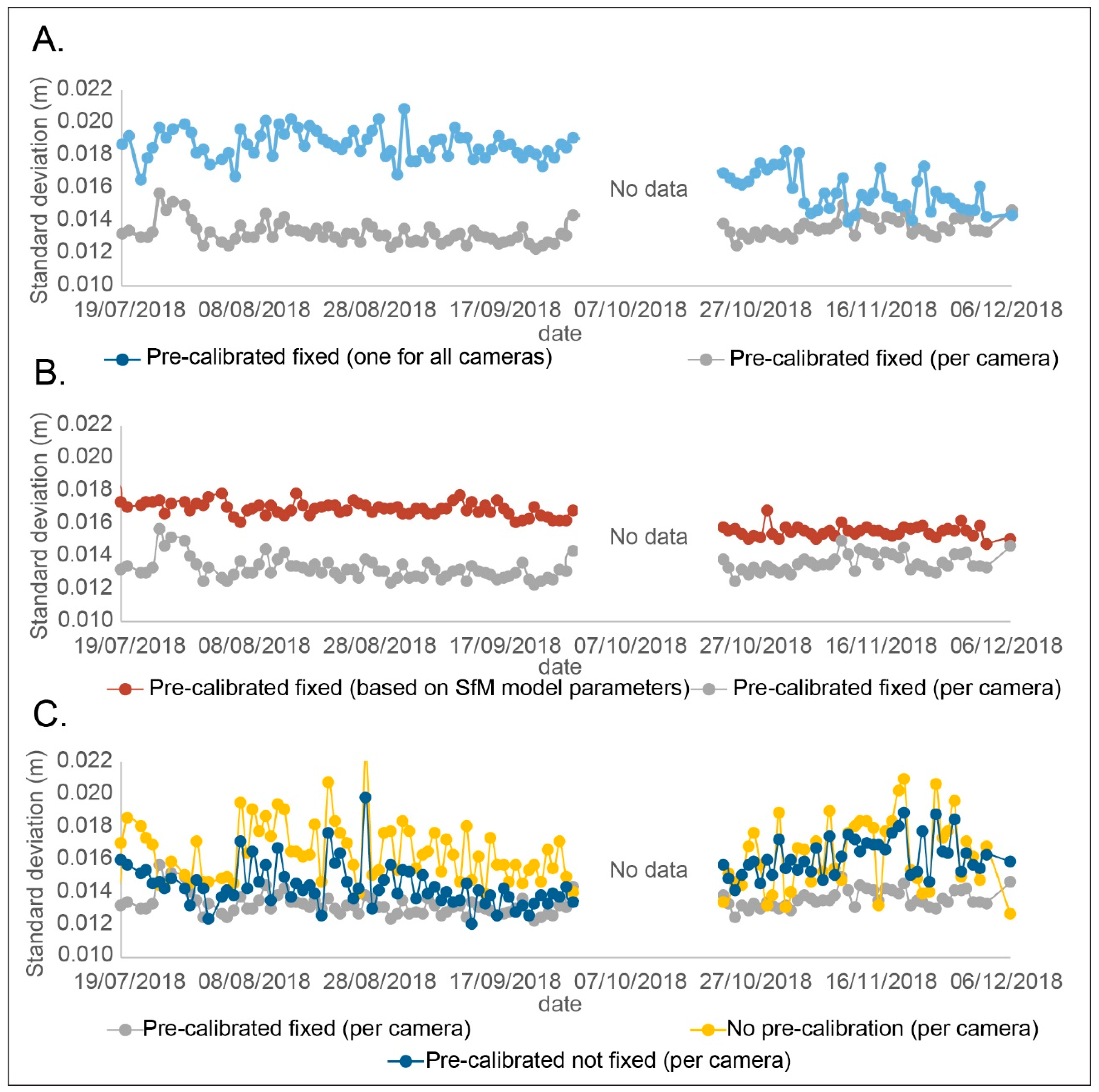
An assessment of spatial accuracy over time was conducted by using the TLS scan as a reference for comparison and calculating the change to each successive SfM model. The standard deviation of the spatial differences is plotted over time in
Figure 9 for three comparison scenarios.
The first comparison scenario (A) shows the difference between using separate fixed pre-calibration parameters for each camera station and using one set of fixed pre-calibration parameters for all cameras (
Figure 9, Inset A). Using separate individual pre-calibration resulted in a better accuracy than using a single calibration for all cameras. The average standard deviations for the time period considered were 0.13 m and 0.16 m, for separate and grouped, respectively.
The second comparison (B) (
Figure 9, Inset B) shows the difference between using separate fixed pre-calibration parameters for each camera station and using separate fixed pre-calibration where the parameters were obtained from a previous SfM model construction. The pre-calibration parameters were obtained by extracting the intrinsic camera parameters of a well-constructed SfM model of the site. The average standard deviation for the pre-calibration from the SfM model was 0.16 m. The pre-calibration based on a SfM model was less accurate than the pre-calibrated case, however, both cases maintained similar precision. The standard deviation of the comparison standard deviations over the time period were 0.0006 m and 0.0008 m for the pre-calibrated fixed models and pre-calibrated fixed model with pre-calibration from a SfM model, respectively.
The third comparison (C) (
Figure 9, Inset C) compared models constructed using a fixed pre-calibration, a non-fixed pre-calibration (intrinsic camera parameters allowed to vary during bundle adjustment), and using no pre-calibration. The fixed pre-calibration performed best in terms of both accuracy and precision. The non-fixed pre-calibration and no pre-calibration were significantly worse in terms of precision (
Table 1). For these two cases, the intrinsic camera parameters were solved during the bundle adjustment. These cases also had outlier cases where a high standard deviation occurred. The outlier cases typically occurred where there was an obstruction in the view in one or multiple photographs, such as a passing transport truck that partially blocked the view, or during poor visibility conditions. The fixed pre-calibration case maintained its precision even in these non-ideal cases. Unless otherwise specified, all following results are presented for the fixed pre-calibration case (with separate pre-calibration for each camera).
6.2. Multiple Combined Photos
Models generated from a fixed network of cameras are produced from a lower number of positions than a traditional terrestrial data collection where one camera can be easily moved to multiple different locations. As result, models are constructed with a low number of photos. To test if increasing the number of photos per station had a positive effect on precision and accuracy of the models in a fixed setup, SfM models were constructed with varying numbers of repeated photos throughout two consecutive days. To estimate precision, models constructed with varying numbers of repeated photos were compared between the two consecutive days. To estimate accuracy models constructed with varying numbers of repeated photos were compared to the TLS model (
Figure 10). Models generated using a greater number of photos produced a better overall precision, however, the accuracy remained between 0.012 and 0.013 m. Although, increasing the number of photos didn’t improve overall accuracy, the combination of photos from different times of day did improve the number of tie points detected in areas obstructed by shadows in individual collections.
6.3. Rockfall Analysis
Change detection results were calculated using the pre-calibrated fixed case without ground control. The rockfalls were extracted from the change detection results and overlaid on the SfM model for comparison.
Figure 11 shows the cumulative amount of rockfalls detected since the beginning of daily monitoring. The rockfalls colored in red highlight the rockfalls that occurred from the TLS baseline scan from 13 February 2018 to the start of photo monitoring on 19 March 2019. More than 50 fragmental rockfalls were detected ranging in size from 0.003 to 0.1 m
3 between 13 February 2018 and 24 June 2019.
A time series deformation analysis was conducted by plotting the per-point change over the study period in the areas where rockfalls occurred. No deformation was detected prior to the rockfalls observed at the site. In this magnitude range, deformation prior to rockfall have been rarely observed [
25].
7. Discussion
A five-camera time lapse camera system was implemented for the long-term monitoring of a rock slope, and an automated data processing workflow was developed that does not require ground control points. This study investigated whether this monitoring method was viable for monitoring rock slope processes and compared the method to one using ground control. The results showed that a well-designed system using a fixed pre-calibration can achieve similar accuracies as methods using ground control. Furthermore, the detection limits achieved were also in the ranges required for monitoring rock slope pre-failure deformation processes and fragmental rockfalls.
This study shows that monitoring using a low number of camera positions in a fixed setup is best done with a network of ground control points. This produces the most accurate models, even when a photo is partially obstructed by an object. However, installing ground control points on a rock slope is not practical nor cost effective. In this study, for example, the installation of ground control targets required the use of climbing ropes and one lane of traffic on the interstate had to be closed.
The results show the importance of pre-calibration in both the creation of spatially accurate models and in its effect at improving model accuracy over a time series, during poor weather conditions or during partial obstruction of the scene. The method developed without using ground control points and using a fixed pre-calibration resulted in similar accuracy and precision as using ground control. This is advantageous as access to the monitored slope is not necessary. Even if some cameras may not require pre-calibration, fixing the intrinsic camera parameters over time can reduce inaccurate model generation due to poor weather, poor lighting conditions, or obstructions within the scene. The network of installed targets was used as a proxy calibration field in this study. The accuracy of the pre-calibration parameters may be further improved by using a separate calibration field. A separate calibration site is also the recommended procedure for using the monitoring methodology without the use of ground control on site.
The time lapse camera system is a viable monitoring approach for rockfall studies, highlighted by over 50 fragmental rockfalls being detected during the study period. Furthermore, using pre-calibration, a level of detection at 95% confidence between 2–3 cm was achieved, which is suitable for detecting pre-failure deformation [
22,
23,
24,
25]. The point clouds generated also provide color data, which facilitates the interpretation of rock slope processes. This is particularly beneficial in discerning the difference between rockfall events and snow melting from the slope.
The suitability of using a time lapse system depends on the site geometry, required level of detection, required frequency of data collection, and budget. In this study, the camera system was built using a budget of USD $ 30000 and allowed the monitoring of an approximately 1600 m2 area of rock slope at a low cm detection level. Similar setups can be used to detect larger movements over a wider area, or smaller movements concentrated over a smaller area.
The method presented was implemented for a rock slope; however, it is also suitable for monitoring many geological processes or civil engineering structures at a variety of timescales. It can be used for monitoring landslides [
18], erosion [
20], debris flows, and construction [
19], for example. In the context of geohazard management, multiple systems could be used and monitored in near-real time at a variety of hazard sites. This could be done with aid of cloud computing. It could allow tracking of hazard events, early warning, and even provide data of the condition of an asset being monitored.
Time lapse monitoring may be unsuitable for some monitoring cases. For example, large areas that require high precision monitoring and a small ground pixel size would require an impractical number of cameras. A feasibility study should be conducted prior to using this method and should consider the required monitoring interval, coverage area, required ground resolution/precision, environmental conditions, and budget. Since the monitoring requires good visibility, environments with frequent precipitation or fog may be unsuitable. More frequent data collection is possible, however, data transfer limits and data processing times should be considered. Furthermore, the system is generally limited to daytime collection. Preliminary tests showed that night time data collection, even with long exposure times, did not provide enough tie points to be able to construct a model accurately. Night time monitoring may be a possibility with artificial light sources.
8. Conclusions
A fixed time lapse camera setup with automated processing was developed to monitor a rock slope on a daily basis. The method does not require the use of ground control points, which is advantageous for studies of near vertical rock cliffs. The method was developed to provide a lower cost monitoring alternative to more expensive technologies such as TLS and GB-InSAR and to provide the capability to monitor geomorphic and geological processes at a high temporal rate.
The results show that it is possible to obtain close to the same accuracy using pre-calibration as with ground control points. The automated processing methods developed in this article can also be used to provide near-real time change data of geological processes. In the context of rock slope hazard management, the system can provide crucial data on the condition of a rock slope, detailed rockfall activity characterization, and areas of potential failure may be detected in advance by monitoring pre-failure deformation. It would be beneficial to apply this monitoring approach to different site geometries and monitoring requirements to further test its feasibility for practical deployment.
Author Contributions
Conceptualization, R.K., G.W., M.L., and R.G.; study site selection, R.K., G.W., R.G.; experiment setup, R.K., B.G., R.G.; method development R.K., B.G.; data analysis R.K.; writing—original draft preparation R.K.; writing—review and editing, R.K., G.W., B.G., M.L.; visualization, R.K., B.G.; project administration, G.W.; funding acquisition, G.W., R.G.
Funding
This research was funded by the Colorado Department of Transportation (CDOT).
Acknowledgments
The authors would like to acknowledge system design advice from Harbortronics, help with target installation from CDOT maintenance crews, I.T. support from the Colorado School of Mines, and BGC engineering for technical support.
Conflicts of Interest
The authors declare no conflict of interest. The funders had a role in the conceptualization of the experiment and in the experimental setup at the field site. The funders had no role in the collection, analyses, or interpretation of data; in writing of the manuscript, or in the decision to publish results.
References
- Lato, M.; Hutchinson, J.; Diederichs, M.; Ball, D.; Harrap, R. Engineering monitoring of rockfall hazards along transportation corridors: Using mobile terrestrial LiDAR. Nat. Hazards Earth Syst. Sci. 2009. [Google Scholar] [CrossRef]
- Abellán, A.; Oppikofer, T.; Jaboyedoff, M.; Rosser, N.J.; Lim, M.; Lato, M.J. Terrestrial laser scanning of rock slope instabilities. Earth Surf. Process. Landf. 2014, 39, 80–97. [Google Scholar] [CrossRef]
- Riquelme, A.J.; Tomás, R.; Abellán, A. Characterization of rock slopes through slope mass rating using 3D point clouds. Int. J. Rock Mech. Min. Sci. 2016, 84, 165–176. [Google Scholar] [CrossRef]
- Bouali, E.H.; Oommen, T.; Vitton, S.; Escobar-Wolf, R.; Brooks, C. Rockfall Hazard Rating System: Benefits of Utilizing Remote Sensing. Environ. Eng. Geosci. 2017, 23, 165–177. [Google Scholar] [CrossRef]
- Jaboyedoff, M.; Oppikofer, T.; Abellán, A.; Derron, M.H.; Loye, A.; Metzger, R.; Pedrazzini, A. Use of LIDAR in landslide investigations: A review. Nat. Hazards 2012, 61, 5–28. [Google Scholar] [CrossRef]
- Westoby, M.J.; Brasington, J.; Glasser, N.F.; Hambrey, M.J.; Reynolds, J.M. “Structure-from-Motion” photogrammetry: A low-cost, effective tool for geoscience applications. Geomorphology 2012, 179, 300–314. [Google Scholar] [CrossRef]
- Eltner, A.; Kaiser, A.; Castillo, C.; Rock, G.; Neugirg, F.; Abellán, A. Image-based surface reconstruction in geomorphometry-merits, limits and developments. Earth Surf. Dyn. 2016, 4, 359–389. [Google Scholar] [CrossRef]
- Haas, F.; Hilger, L.; Neugirg, F.; Umstädter, K.; Breitung, C.; Fischer, P.; Hilger, P.; Heckmann, T.; Dusik, J.; Kaiser, A.; et al. Quantification and analysis of geomorphic processes on a recultivated iron ore mine on the Italian island of Elba using long-term ground-based lidar and photogrammetric SfM data by a UAV. Nat. Hazards Earth Syst. Sci. 2016, 16, 1269–1288. [Google Scholar] [CrossRef]
- Cucchiaro, S.; Maset, E.; Fusiello, A.; Cazorzi, F. 4D-SFM photogrammetry for monitoring sediment dynamics in a debris-flow catchment: Software testing and results comparison. Int. Arch. Photogramm. Remote Sens. Spat. Inf. Sci. 2018, 42, 281–288. [Google Scholar] [CrossRef]
- Bozzano, F.; Mazzanti, P.; Prestininzi, A.; Mugnozza, G.S. Research and development of advanced technologies for landslide hazard analysis in Italy. Landslides 2010, 7, 381–385. [Google Scholar] [CrossRef]
- Barla, M.; Antolini, F.; Bertolo, D.; Thuegaz, P.; D’Aria, D.; Amoroso, G. Remote monitoring of the Comba Citrin landslide using discontinuous GBInSAR campaigns. Eng. Geol. 2017, 222, 111–123. [Google Scholar] [CrossRef]
- Dick, G.J.; Eberhardt, E.; Cabrejo-Liévano, A.G.; Stead, D.; Rose, N.D. Development of an early-warning time-of-failure analysis methodology for open-pit mine slopes utilizing ground-based slope stability radar monitoring data. Can. Geotech. J. 2014, 52, 515–529. [Google Scholar] [CrossRef]
- Rouyet, L.; Kristensen, L.; Derron, M.H.; Michoud, C.; Blikra, L.H.; Jaboyedoff, M.; Lauknes, T.R. Evidence of rock slope breathing using ground-based InSAR. Geomorphology 2017, 289, 152–169. [Google Scholar] [CrossRef]
- Atzeni, C.; Barla, M.; Pieraccini, M.; Antolini, F. Early Warning Monitoring of Natural and Engineered Slopes with Ground-Based Synthetic-Aperture Radar. Rock Mech. Rock Eng. 2015, 48, 235–246. [Google Scholar] [CrossRef]
- Kromer, R.A.; Abellán, A.; Hutchinson, D.J.; Lato, M.; Chanut, M.A.; Dubois, L.; Jaboyedoff, M. Automated terrestrial laser scanning with near-real-time change detection—Monitoring of the Séchilienne landslide. Earth Surf. Dyn. 2017, 5, 293–310. [Google Scholar] [CrossRef]
- Williams, J.G.; Rosser, N.J.; Hardy, R.J.; Brain, M.J.; Afana, A.A. Optimising 4-D surface change detection: An approach for capturing rockfall magnitude-frequency. Earth Surf. Dyn. 2018, 6, 101–119. [Google Scholar] [CrossRef]
- Van Veen, M.; Hutchinson, D.J.; Kromer, R.; Lato, M.; Edwards, T. Effects of sampling interval on the frequency—Magnitude relationship of rockfalls detected from terrestrial laser scanning using semi-automated methods. Landslides 2017, 14, 1579–1592. [Google Scholar] [CrossRef]
- Roncella, R.; Forlani, G. A Fixed Terrestrial Photogrammetric System for Landslide Monitoring. In Modern Technologies for Landslide Monitoring and Prediction; Springer: Berlin/Heidelberg, Germany, 2015. [Google Scholar]
- Santise, M.; Thoeni, K.; Roncella, R.; Sloan, S.W.; Giacomini, A. Preliminary tests of a new low-cost photogrammetric system. Int. Arch. Photogramm. Remote Sens. Spat. Inf. Sci. 2017, 42, 229. [Google Scholar] [CrossRef]
- Eltner, A.; Kaiser, A.; Abellan, A.; Schindewolf, M. Time lapse structure-from-motion photogrammetry for continuous geomorphic monitoring. Earth Surf. Process. Landf. 2017, 42, 2240–2253. [Google Scholar] [CrossRef]
- Parente, L.; Chandler, J.; Dixon, N. Precise change detection despite inaccurate camera calibration. In Proceedings of the 3rd Virtual Geoscience Conference, Kingston, ON, Canada, 22–24 August 2018; pp. 60–61. [Google Scholar]
- Abellán, A.; Calvet, J.; Vilaplana, J.M.; Blanchard, J. Detection and spatial prediction of rockfalls by means of terrestrial laser scanner monitoring. Geomorphology 2010, 119, 162–171. [Google Scholar] [CrossRef]
- Royán, M.J.; Abellán, A.; Jaboyedoff, M.; Vilaplana, J.M.; Calvet, J. Spatio-temporal analysis of rockfall pre-failure deformation using Terrestrial LiDAR. Landslides 2014, 11, 697–709. [Google Scholar] [CrossRef]
- Kromer, R.A.; Hutchinson, D.J.; Lato, M.J.; Gauthier, D.; Edwards, T. Identifying rock slope failure precursors using LiDAR for transportation corridor hazard management. Eng. Geol. 2015, 195, 93–103. [Google Scholar] [CrossRef]
- Kromer, R.A.; Rowe, E.; Hutchinson, J.; Lato, M.; Abellán, A. Rockfall risk management using a pre-failure deformation database. Landslides 2018, 15, 847–858. [Google Scholar] [CrossRef]
- Esri; Garmin; USGS; NPS. World Reference Overlay. Created 2009, Updated 2019. Available online: https://server.arcgisonline.com/ArcGIS/rest/services/Reference/World_Reference_Overlay/MapServer (accessed on 8 January 2019).
- Moench, R.H.; Avery, D.A.J. Economic Geology of the Idaho Springs District Clear Creek and Gilpin Counties, Colorado, Geological Survey Bulletin 1208, prepared on behalf of US Atomic Energy Commission; United States Government Printing Office: Washington, DC, USA, 1966.
- Harrison, J.E.; Moench, R.H. Joints in Precambrian Rocks, Central City-Idaho Springs Area, Colorado: U.S. Geol. Survey Prof. Paper 374-B, prepared on behalf of US Atomic Energy Commission; United States Government Printing Office: Washington, DC, USA, 1961.
- Harbortronics Cyclapse Time Lapse Camera System 2018. Available online: https://cyclapse.com (accessed on 6 July 2019).
- Dai, F.; Lu, M. Three-Dimensional Modeling of Site Elements by Analytically Processing Image Data Contained in Site Photos. J. Constr. Eng. Manag. 2012, 139, 881–894. [Google Scholar] [CrossRef]
- Agisoft LLC Agisoft PhotoScan Professional. 2019. Available online: http://www.Agisoft.Ru/Products/Photoscan/Professional/ (accessed on 6 July 2019).
- Python (version 3.7.3). 2019. Available online: https://www.python.org/downloads/ (accessed on 6 July 2019).
- Bae, K.H.; Lichti, D.D. A method for automated registration of unorganised point clouds. ISPRS J. Photogramm. Remote Sens. 2008, 63, 36–54. [Google Scholar] [CrossRef]
- Theiler, P.W.; Schindler, K. Automatic registration of terrestrial laser scanner point clouds using natural planar surfaces. ISPRS Ann. Photogramm. Remote Sens. Spat. Inf. Sci. 2012, 3, 173–178. [Google Scholar] [CrossRef]
- Theiler, P.W.; Wegner, J.D.; Schindler, K. Keypoint-based 4-Points Congruent Sets—Automated marker-less registration of laser scans. ISPRS J. Photogramm. Remote Sens. 2014, 96, 149–163. [Google Scholar] [CrossRef]
- Holz, D.; Ichim, A.E.; Tombari, F.; Rusu, R.B.; Behnke, S. Registration with the point cloud library: A modular framework for aligning in 3-D. IEEE Robot. Autom. Mag. 2015, 22, 110–124. [Google Scholar] [CrossRef]
- Novák, D.; Schindler, K. Approximate registration of point clouds with large scale differences. ISPRS Ann. Photogramm. Remote Sens. Spat. Inf. Sci. 2013, 1, 211–216. [Google Scholar] [CrossRef]
- Persad, R.A.; Armenakis, C. Automatic co-registration of 3D multi-sensor point clouds. ISPRS J. Photogramm. Remote Sens. 2017, 130, 162–186. [Google Scholar] [CrossRef]
- Palma, G.; Boubekeur, T.; Ganovelli, F.; Cignoni, P. Scalable non-rigid registration for multi-view stereo data. ISPRS J. Photogramm. Remote Sens. 2018, 142, 328–341. [Google Scholar] [CrossRef]
© 2019 by the authors. Licensee MDPI, Basel, Switzerland. This article is an open access article distributed under the terms and conditions of the Creative Commons Attribution (CC BY) license (http://creativecommons.org/licenses/by/4.0/).


