Mapping Crop Residue by Combining Landsat and WorldView-3 Satellite Imagery

Abstract

A unique, multi-tiered approach was applied to map crop residue cover on the Eastern Shore of the Chesapeake Bay, United States. Field measurements of crop residue cover were used to calibrate residue mapping using shortwave infrared (SWIR) indices derived from WorldView-3 imagery for a 12-km × 12-km footprint. The resulting map was then used to calibrate and subsequently classify crop residue mapping using Landsat imagery at a larger spatial resolution and extent. This manuscript describes how the method was applied and presents results in the form of crop residue cover maps, validation statistics, and quantification of conservation tillage implementation in the agricultural landscape. Overall accuracy for maps derived from Landsat 7 and Landsat 8 were comparable at roughly 92% (+/− 10%). Tillage class-specific accuracy was also strong and ranged from 75% to 99%. The approach, which employed a 12-band image stack of six tillage spectral indices and six individual Landsat bands, was shown to be adaptable to variable soil moisture conditions—under dry conditions (Landsat 7, 14 May 2015) the majority of predictive power was attributed to SWIR indices, and under wet conditions (Landsat 8, 22 May 2015) single band reflectance values were more effective at explaining variability in residue cover. Summary statistics of resulting tillage class occurrence matched closely with conservation tillage implementation totals reported by Maryland and Delaware to the Chesapeake Bay Program. This hybrid method combining WorldView-3 and Landsat imagery sources shows promise for monitoring progress in the adoption of conservation tillage practices and for describing crop residue outcomes associated with a variety of agricultural management practices.

1. Introduction

Conservation tillage, which can be defined as any form of tillage that minimizes tillage intensity and maintains crop residue on the soil surface, is a best management practice with well-documented benefits to agricultural ecosystems. Some of these benefits include reduced runoff and soil erosion, increased infiltration and aggregate stability, greater soil carbon accumulation, enhanced soil health, and improved water quality in neighboring water bodies [1,2,3]. The use of conservation tillage has been incentivized throughout the United States by the U.S. Department of Agriculture Natural Resources Conservation Service, and the practice is often adopted to meet conservation requirements for highly erodible lands [4]. In the Chesapeake Bay watershed, where reductions in agricultural runoff and erosion can have substantial benefits to the health of the Chesapeake Bay estuary [5], conservation tillage has been identified as a primary strategy for reducing loss of sediment from farmland. Accordingly, conservation tillage has been incentivized throughout the Chesapeake Bay watershed. The effects of this practice, in combination with a broad suite of improvements to agricultural and point-source pollution management strategies, have had a gradual influence on improving the health of the Chesapeake Bay. For example, in a 2015 analysis, decreases in long-term trends of nitrogen loads were observed at a majority of observation stations, while trends toward improved phosphorous and suspended-sediment loads were reported in a third of observation stations [6]. Chesapeake Bay water clarity and dissolved oxygen have also improved since 2014, an indicator of gradually improving estuary health that is partially attributed to increased implementation of agricultural conservation practices, including conservation tillage [5].

Three tillage intensity classes are of particular interest for monitoring percent crop residue cover (CRC): conventional or low-residue tillage (0–30% CRC), conservation tillage (30–60% CRC), and high-residue, minimum soil disturbance tillage management (60–100% CRC) [7,8]. A 2013 survey of Maryland farmers indicated that in corn, soybean, winter wheat, and barley fields, no-till management practices were adopted in 71% of fields, conservation tillage in 21.3% of fields, and conventional tillage in 7.7% of fields [9]. Alongside such surveys, the Maryland Department of Agriculture is interested in mapping CRC for the entire state. However, covering a large area such as the state of Maryland using traditional methods, such as line-point transects or roadside surveys, would be time consuming and costly. Consequently, the use of remote sensing and satellite imagery is a pragmatic method for monitoring tillage practices statewide. Maps derived from satellite remote sensing would enhance the accuracy and precision of tillage management statistics and would enable the tracking of tillage practices over time and space. Landsat imagery provides useful data to support the mapping of CRC at the landscape scale, due to its moderate spatial resolution of 30 m, large swath width of 185 km, and no-cost availability.

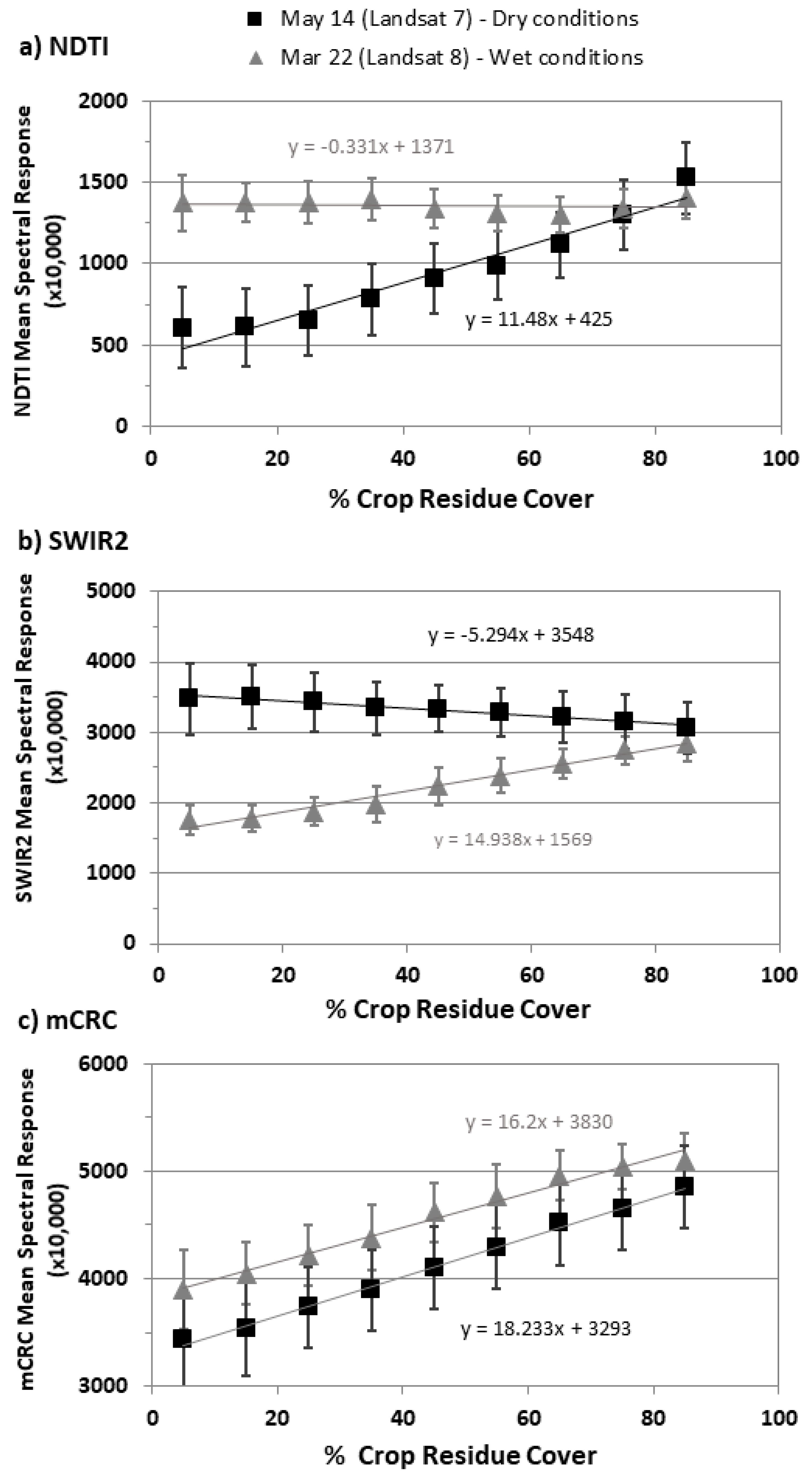
Remote sensing using Landsat imagery has been previously used in multiple studies with varying methods to monitor crop residue conditions [3,8,10,11,12,13]. A review of methods is provided in Zheng et al. [14] and in Bégué et al. [15]. Because soils and residues are spectrally similar in the visible and near infrared, the most successful Landsat-based tillage indices tend to exploit contrasts between the two broad Landsat shortwave infrared (SWIR) bands, SWIR1: 1550–1750 nm and SWIR2: 2090–2350 nm. Despite their successes, these indices are reliant on the relative differences in reflectance that occur between crop residue and soils in each Landsat scene, and changes in soil moisture conditions can have profound effects on how an index performs [10,16,17]. Increasing moisture content reduces reflectance from the visible to the shortwave infrared and attenuates reflectance features, shifting the relationship between the two broad Landsat SWIR bands. This can lead to the overestimation of CRC under wet conditions [17]. The contrasts provided by the broadband Landsat indices are also influenced by crop residue age and condition, soil brightness, and the presence of green vegetation [10,14], which can sometimes limit their effectiveness. To be accurate, all methods relying upon the broad contrasts provided by Landsat reflectance bands require the collection of ground-truth (end-member) data to calibrate to the particular conditions in a scene [18], particularly with respect to soil moisture conditions.

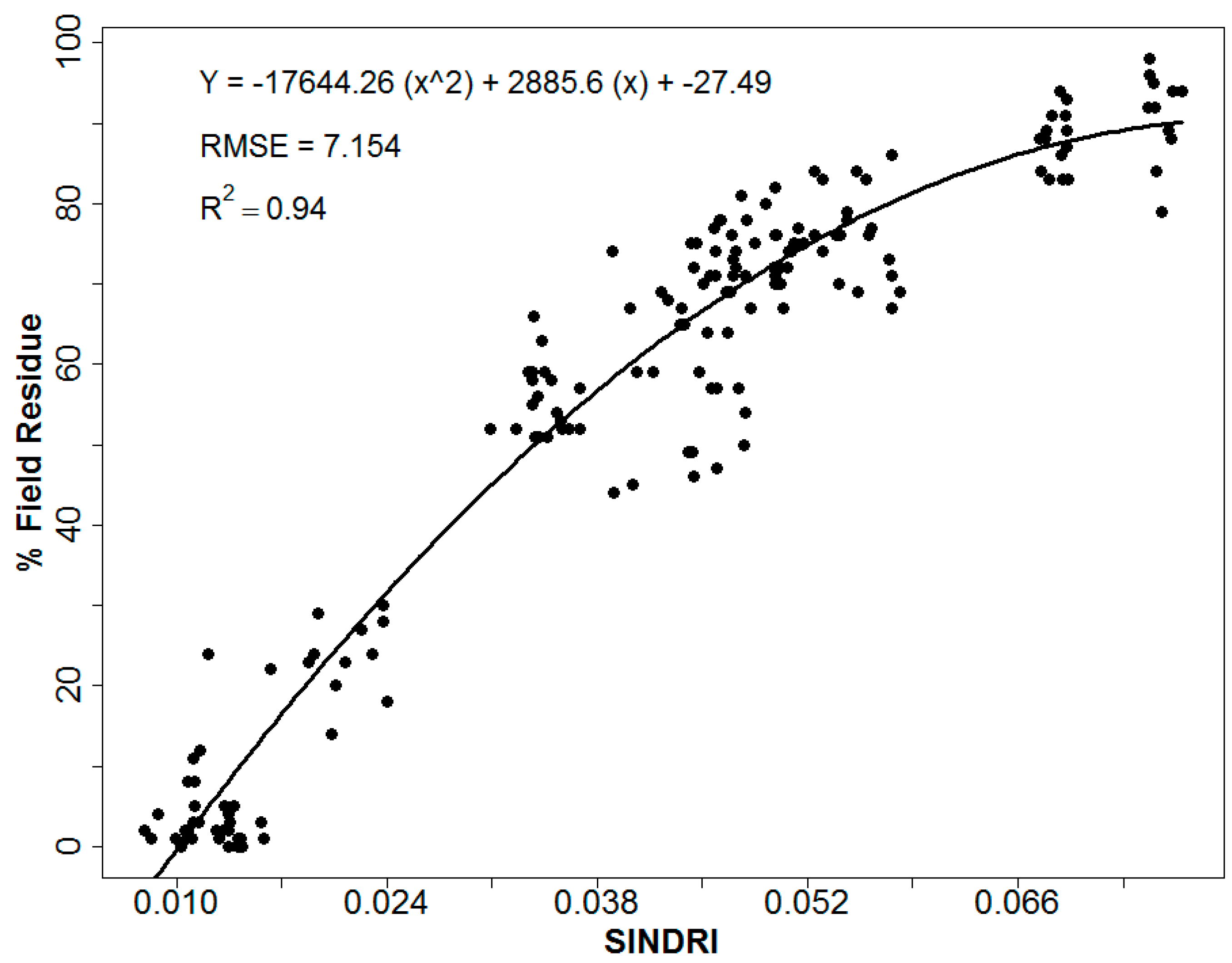
Hyperspectral indices, such as the Cellulose Absorption Index (CAI), and its narrow-band analog the Shortwave Infrared Normalized Difference Residue Index (SINDRI), have demonstrated increased accuracy for measurement of CRC in comparison to Landsat-based indices, because they measure a narrow SWIR adsorption feature, observed near 2100 nm, that is associated with the cellulose and lignin content of crop residues [8,19]. Calculation of these indices relies upon the spectral resolution provided by proximal or airborne hyperspectral instruments [10] or by the WorldView-3 satellite [20]. However, under wet conditions the distinctness of the cellulose–lignin peak becomes muted [21] and the narrowband SWIR indices can also exhibit reduced effectiveness unless well-calibrated [10] or adjusted for moisture conditions [17].

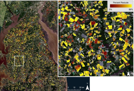
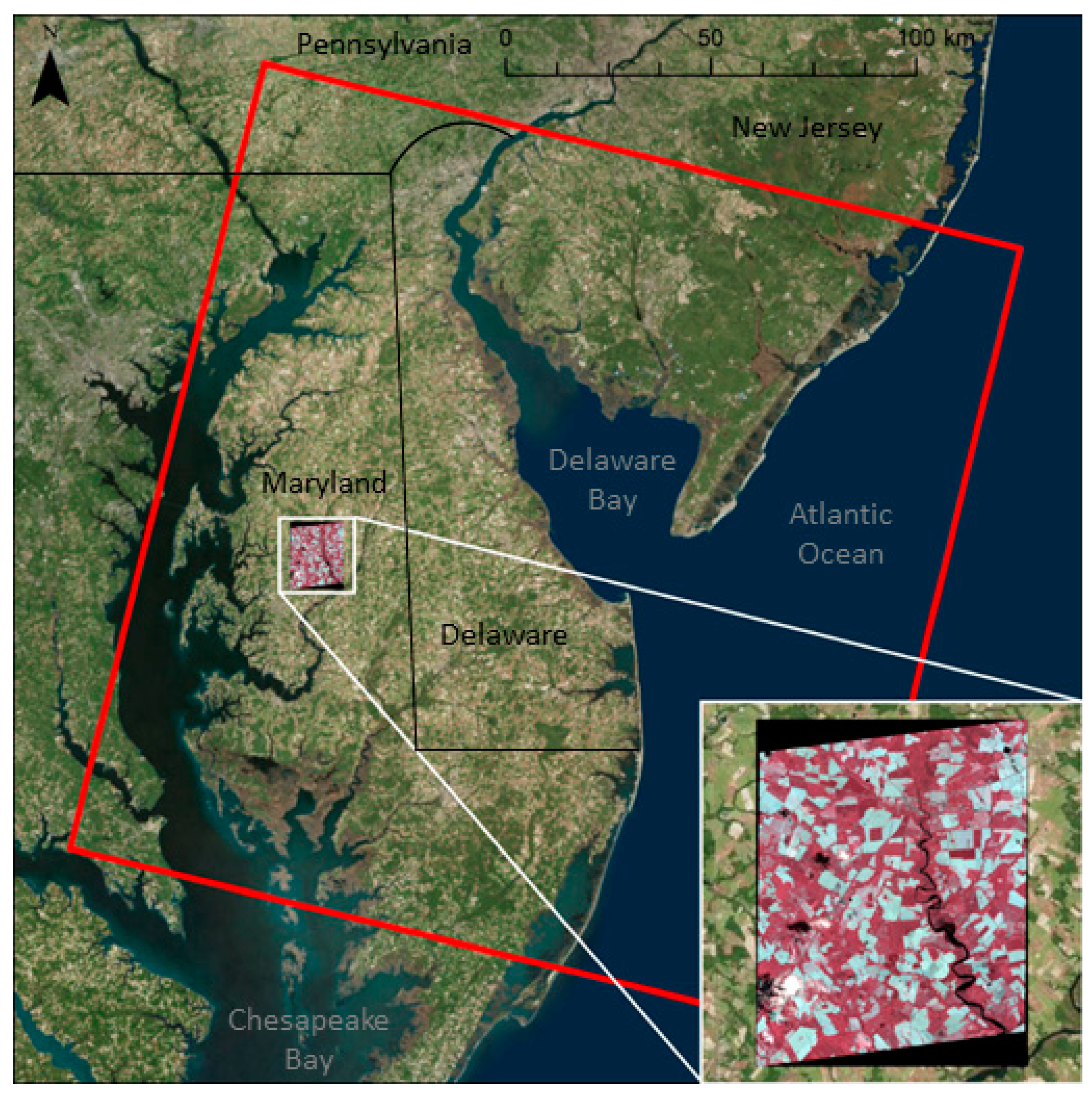
This manuscript describes a unique approach that combined a field sampling campaign, high-resolution WorldView-3 (WV3) SWIR imagery, and moderate-resolution Landsat imagery to monitor crop residue conditions over the Eastern Shore of the Chesapeake Bay. Previous research from Hively et al. [20] demonstrated a strong correlation (R² = 0.94, RMSE = 7.14) between CRC and the WV3 derived SINDRI index and used this relationship to map CRC on non-vegetated crop fields throughout the extent of the WV3 imagery footprint. We propose that the well-calibrated map of CRC derived in Hively et al. [20] can be used to provide a sufficient volume of ground-truth calibration data to train a Landsat-based Gradient Boosting Tree classifier to map CRC at a large spatial extent, using temporally adjacent Landsat imagery. Unlike previous research relying on single spectral indices, this research combines the six Landsat reflectance bands in the visible to SWIR portion of the electromagnetic spectrum with six derived broadband spectral indices to create a 12-band image stack and employs gradient boosting trees to derive an optimal CRC map. Using multiple bands and indices enables the classifier to evaluate which bands perform the best under variable soil moisture conditions and reduces the impact of rainfall events on classification accuracy.

2. Materials and Methods

2.1. Site Location and Satellite Imagery Acquisition

Field sampling took place on a collaborating farm located in the Choptank River watershed, Talbot County, MD, United States, on 15 May 2015. WV3 satellite imagery was acquired for this region a day before field sampling. Clear Landsat imagery was also acquired for the Delmarva Peninsula and included portions of Maryland, the state of Delaware, southern New Jersey, and southeastern Pennsylvania (Figure 1) on 14 May 2015 (Landsat 7) and 22 May 2015 (Landsat 8). According to the U.S. Department of Agriculture Soil Taxonomy classification [22], the primary soil order in this area is ultisols, typified by the Othello soil series (fine-silty, mixed, active, mesic typic endoaquults) and the Mattapex soil series (fine-silty, mixed, active, mesic aquic hapludults). Othello soils are poorly drained with moderately slow permeability and Mattapex soils are moderately well-drained with moderate permeability. Coastal entisols, organic histosols and alfisols are also present within the study area.

WorldView-3 satellite imagery from 14 May 2015, was obtained and delivered as 8 bands of visible and near infrared (VIS/NIR) at 2-m spatial resolution and 8 bands of SWIR at 4-m spatial resolution. The imagery was converted from Digital Number (DN) to top-of-atmosphere radiance and then atmospherically corrected to surface reflectance values using the MODerate resolution atmospheric TRAnsmission (MODTRAN) computer code version 5.4. VIS/NIR bands were then resampled to a 4-m spatial resolution and co-registered to the SWIR bands using nearest-neighbor interpolation. The footprint of this image was 12 km × 12 km. Any clouds were individually masked by hand.

Two predominantly cloud-free Landsat images were also acquired for the Eastern Shore of the Chesapeake Bay in Worldwide Reference System 2 (WRS-2) path/row 14/33. The first image was a Landsat 7 Enhanced Thematic Mapper+ (ETM+) scene from 14 May 2015. This scene was atmospherically corrected to surface reflectance using the Landsat Ecosystem Disturbance Adaptive Processing System (LEDAPS) [23] and downloaded from Earth Explorer (https://earthexplorer.usgs.gov/) as a Collection-1 Level-2 product (imagery filename: LE07_L1TP_014033_20150514_20160902_01_T1). An additional Landsat 8 Operational Land Imager (OLI) scene from 22 May 2015 was also acquired and atmospherically corrected to surface reflectance using the Landsat 8 Surface Reflectance (L8SR) system [24,25], and was downloaded from Earth Explorer as a Collection-1 Level-2 product (imagery filename: LC08_L1TP_014033_20150522_20170226_01_T1). Both images were referenced in Universal Transverse Mercator (UTM) coordinates and clouds were masked out using the 2015 updated version of Fmask [26].

2.2. Soil Moisture Data

Because crop residue conditions were being monitored across two separate dates of Landsat imagery, it was necessary to measure soil moisture to ensure that differences in output maps could be understood. Soil-water content has been shown to affect the ability to map CRC [27]. For some tillage indices, previous research has indicated that dry conditions are optimal for mapping [10]. Conditions on 14 May were generally dry, as was evidenced by the activation of nine center pivot irrigation units within the 12-km × 12-km WorldView-3 imagery extent [17]. While the non-irrigated landscape was generally dry, higher wetness conditions were present in fields receiving irrigation. Between that date and the 22 May Landsat 8 overpass, one of the largest rainfall events of the spring occurred (cumulative precipitation amount of 93.6 mm). Observing how this rainfall affected the monitoring of crop residue conditions was critical to understanding how Landsat surface reflectance bands and derived tillage indices functioned under differing soil moisture conditions.

Ten on-farm weather stations are situated across the Choptank River basin (http://hrsl.arsusda.gov/lcb/data.php), one located within the WV3 imagery footprint. Each of these stations measures precipitation (mm of rainfall) using a 10-cm-diameter tipping bucket rain gauge, and measures electrical conductance at 10 cm depth to determine soil volumetric moisture content using a Stevens Hydra Probe.

Table 1. Average estimated rainfall and soil volumetric moisture content from 10 weather stations situated within the Choptank River basin, May 2015.

Date	Rainfall (mm)	Soil Moisture (%)
1–9 May	<3	10.0
10-May	1.5	9.4
11-May	0.5	8.9
14-May *	0.3	7.9
16-May	7.6	7.6
17-May	6.9	10.5
18-May	42.2	10.0
19-May	21.1	21.1
21-May	15.5	15.8
22-May **	0.1	21.9

* Landsat 7 and WV3 imagery acquisition; ** Landsat 8 imagery acquisition.

describes rainfall events and soil moisture conditions derived as the average of the 10 stations.

2.3. Field Sampling

Field sampling occurred on a collaborating grain farm on the Eastern Shore of Maryland on 15 May 2015, as described by Hively et. al. [20]. Ten agricultural fields were sampled with various tillage management ranging from plow tillage (0% residue) to no-till (>84% residue). Vertical downward-looking photographs were collected from a height of 2 m (sampling approximately 4 m² of field surface) at >10 locations per field. The 174 resulting photographs were processed by using Sample Point software (www.samplepoint.org) to categorize percent residue cover. Within each photograph, cover types beneath 144 randomly placed points were manually characterized into one of three categories (crop residue, soil, or vegetation) by visual inspection, and these data were used to derive an estimated percent CRC for each sampling location. These photo-derived CRC data matched closely to in-field measurements collected using the traditional point-transect method [10].

2.4. Calculation of SINDRI and Transformation to Crop Residue Cover

WorldView-3 surface reflectance imagery collected on 14 March 2015, was used to calculate the Shortwave Infrared Normalized Difference Residue Index (SINDRI) [19,28] for the image extent:

SINDRI = (SWIR6 − SWIR7)/(SWIR6 + SWIR7)

(1)

using the SWIR6 band centered at 2202 nm and the SWIR7 band centered at 2259 nm.

Using the same field sampling dataset described in this study, Hively et al. [20] documented the effectiveness of nine SWIR indices for mapping crop residue and found that the SINDRI was the most accurate (highest goodness of fit, lowest residual error; Figure 2). The SINDRI is robust as it targets the 2150 nm cellulose absorption feature that is specific to crop residue [19], enabling effective mapping and separation from soil. Additionally, this index has been shown to be resistant to soil moisture [10,17], decomposition stage of crop residue [27], and interference from low levels of green vegetation [20]. Thus, SINDRI was chosen to map crop residue conditions at WV3 extent and spatial resolution.

The WV3 SINDRI raster was transformed to a map of CRC using a second order polynomial equation derived in Hively et al. [20] based on correlation with field sampling data, with an R² value of 0.94 and root mean square error (RMSE) of 7.15. In this WV3 image, saturation of the second order polynomial occurred around 88% crop residue cover. Thus, any mapped values of 88% are representative of high crop residue cover values that range from 88–100% CRC.

2.5. Calculation of Landsat Indices and Creation of an Imagery Stack

A 12-band image stack of Landsat spectral bands and tillage indices was created to monitor crop residue conditions at Landsat extent and spatial resolution. The stack included six Landsat surface reflectance bands (Blue, Green, Red, NIR, SWIR1, SWIR2) and six tillage indices derived from those bands that have previously been shown to be effective at monitoring crop residue conditions (

Table 2. Summary table describing Landsat-derived reflectance indices, their formulas, and associated references. The spectral profiles of the Landsat bands are as follows: Blue (0.45–0.52 μm), Green (0.52–0.60 μm), Red (0.63–0.69 μm), NIR (0.77–0.90 μm), SWIR1 (1.55–1.75 μm), and SWIR2 (2.09–2.35 μm). These six bands correspond to Landsat 8 (OLI) bands 2–7 or Landsat 7 ETM+ bands 1–5, and 7. The indices included the Normalized Difference Indices 5 and 7 (NDI5, NDI7), the Normalized Difference Senescent Vegetation Index (NDSVI), the Normalized Difference Tillage Index (NDTI), the Simple Tillage Index (STI), and the Modified Crop Residue Cover (mCRC) index.

Reflectance Index	Formula	Reference
NDI5	(NIR − SWIR1)/(NIR + SWIR1)	McNairn and Protz [29]
NDI7	(NIR − SWIR2)/(NIR + SWIR2)	McNairn and Protz [29]
NDSVI	(SWIR1 − Red)/(SWIR1 + Red)	Qi et al. [30]
NDTI	(SWIR1 − SWIR2)/(SWIR1 + SWIR2)	Van Deventer et al. [13]
STI	(SWIR1)/(SWIR2)	Van Deventer et al. [13]
mCRC	(SWIR1 − Green)/(SWIR1 + Green)	Sullivan et al. [1,12]

). The spectral profiles of the Landsat bands are as follows: Blue (0.45–0.52 μm), Green (0.52–0.60 μm), Red (0.63–0.69 μm), NIR (0.77–0.90 μm), SWIR1 (1.55–1.75 μm), and SWIR2 (2.09–2.35 μm), corresponding respectively to Landsat 8 (OLI) bands 2–7 or Landsat 7 (ETM+) bands 1–5, and 7. The indices included the Normalized Difference Indices 5 and 7 (NDI5 [29], NDI7 [29]), the Normalized Difference Senescent Vegetation Index (NDSVI [30]), Normalized Difference Tillage Index (NDTI [13]), the Simple Tillage Index (STI [13]), and the Modified Crop Residue Cover (mCRC) index [1,12].

Four green vegetation indices were also tested for inclusion in the analysis, including the Normalized Difference Vegetation Index (NDVI) [31], Optimized Soil-Adjusted Vegetation Index (OSAVI) [32], Visible Atmospherically Resistant Index (VARI) [33], and the Green Vegetation Index (VIGreen) [34,35]. However, these indices were shown to be less effective at representing crop residue cover (accuracy < 50%), added little to no value to the analysis, and were therefore discarded. This finding is in agreement with previous research indicating that crop residue cover is not well correlated with any of the green vegetative indices [33].

2.6. Masking Landsat Imagery to Non-Vegetated Croplands

The Landsat 7 and Landsat 8 images were developed as cloud-masked surface reflectance and were subsequently masked to include only agricultural areas (cropland, grassland, and pasture) using the 2015 Cropland Data Layer [36] and the 2011 National Land Cover Database [37]. Grassland and pasture areas were included because it was suspected that agricultural croplands could be easily misclassified as either of these categories. To limit analysis to crop fields with minimal vegetation, the images were masked to include only pixels with NDVI values < 0.3. This reduced the spectral interference of green vegetation, such as emergent corn and soybean crops, and masked out true grassland and pasture areas, which tend to maintain NDVI > 0.3 throughout the year [38]. The NDVI [31] was calculated as:

NDVI = (NIR − Red)/(NIR + Red)

(2)

In addition to the agricultural lands and NDVI masks, a mask was also applied to remove water-covered areas using the Dynamic Surface Water Extent product [39]. Any pixel that was identified as open water during a calendar year was masked out. Finally, pixels falling under the scan line error were removed from the Landsat 7 scene. The net result was a 12-band raster image for each Landsat date containing six reflectance bands and six reflectance indices, covering only agricultural fields with minimal vegetation. These datasets were used for Landsat-based crop residue analysis. In total, in the Landsat 7 scene, about 74.3% of the surface area was masked out, as compared to 69.5% of the Landsat 8 scene.

To evaluate the effect of precipitation on soil moisture conditions, a Wetness Index (WI) [17] was calculated for each of the Landsat scenes:

WI = SWIR1/SWIR2

(3)

2.7. Creating a Calibration Dataset and Training a Classifier

The 4-m resolution map of calculated percent residue cover that was derived from 14 May 2015, WV3 SWIR imagery in Hively et. al [20], covering the 12-km × 12-km footprint of the WV3 acquisition (Figure 3), was masked to agricultural fields with minimal vegetation using Common Land Unit polygons [40] to identify agricultural fields and a threshold of NDVI < 0.3 to identify minimally vegetated areas. This residue map was resampled to 30 m, representing the average percent residue cover values of all 4-m pixels within each 30 m, and was snapped to Landsat pixel locations to serve as a training dataset for Landsat analysis. The WV3-derived percent residue cover values were binned into groups of 10% (0–10%, 10–20%, …, 80–90%) to reduce computational intensity and improve classification quality.

The 30-m pixels within the resampled WV3 crop residue map were randomly split 50:50 to define calibration and validation datasets. The Landsat classifiers were trained on the calibration data and tested on the validation data. A Gradient Boosting Tree (GBT) classifier [41] was employed to classify each Landsat 12-band image stack into a percent residue cover map. The GBT classifier was chosen after testing because it was shown to be markedly superior in terms of overall accuracy and class-specific accuracies when compared to other tested classifiers, which included the Decision Tree classifier, k-nearest neighbor classifier, and Naive Bayes classifier (results not shown). The GBT, and each classifier tested, was optimized to parameters that would minimize overfitting, yet produce the best possible results (

Table 3. Summary table describing the chosen parameters for the Gradient Boosting Tree classifier (GBT).

Parameter	Value
Training and validation sample ratio	50:50
Number of boosting algorithm iterations	750
Portion of the training dataset used for each iteration	50%
Maximum depth of tree	8
Regularization parameter	0.01
Maximum training/validation sample size per class	unlimited

). To optimize, a grid search was used to evaluate performance using a random subset of the data, while varying the number of boosting algorithm iterations (250, 500, 750, and 1000), the maximum depth of the tree (4 to 8), and the portion of training data used for each iteration (25%, 50%, and 75%). Overfitting was avoided by using L2 regularization to penalize the complexity of the tree. These methods and parameters follow suggested settings that have been found to produce accurate results while minimizing overfitting of the data [41,42].

Maps of predicted percent crop residue cover were derived for each of the Landsat images by applying the GBT classifier to the 12-band Landsat image stack using training data from the WV3-derived calibration dataset. Each of these maps depicts the percentage of crop residue cover on non-vegetated agricultural fields, at Landsat extent and spatial resolution. The accuracy and comparison of these products were described using fuzzy confusion matrices. True positive accuracy was determined using the main diagonal of the confusion matrices, with an accurate match determined as +/− 10% (exact match plus adjacent 10% crop residue bin).

In addition to mapping crop residue cover using the 12-band stack, each of the individual bands that contributed to the stack was used as a single input to the same standardized GBT classifier framework, using only one band at a time for input, and using the optimized coefficients listed in Table 3. This enabled comparisons of how much each band contributed to the crop residue classification and how much soil moisture conditions affected results.

2.8. Comparison with State Jurisdictional Datasets

Currently, Maryland reports conservation tillage implementation based upon farmer self-reporting in annual farmland management surveys [43], and Delaware reports conservation tillage implementation based upon annual springtime driving roadside surveys [44]. These data are reported to the Chesapeake Bay Program Partnership in December of each year and are incorporated into the Chesapeake Bay water-quality modeling. For comparison with remote sensing results, the Maryland reported data for 2015 were obtained from the Chesapeake Assessment Scenario Tool (CAST) [43] and the Delaware Survey data were obtained from the Delaware Department of Natural Resources and Environmental Control [44].

3. Results and Discussion

3.1. Landsat 7 Enhanced Thematic Mapper (ETM+) Map of Crop Residue Cover

The 14 May 2015, Landsat 7 map of percent crop residue cover (Figure 4), when compared to the validation dataset, exhibited an overall accuracy of 93.3% of classifications falling within +/− 10% of the “true” classification, as described in a fuzzy confusion matrix (

Table 4. Confusion matrix showing Landsat 7 predicted crop residue cover compared to validation data derived from the WorldView-3 imagery classification. Pixels that are described as accurate (+/− one residue class) are colored red in the confusion matrix. Inaccurate pixels are colored black.

		Classified % Residue Cover										Producer Accuracy
		0–10	10–20	20–30	30–40	40–50	50–60	60–70	70–80	80–90	Totals
Reference % Residue Cover	0–10	563	143	62	23	9	2	2	1	1	806	87.6%
	10–20	159	283	102	20	5	3	0	0	1	573	94.9%
	20–30	42	100	285	85	6	3	2	0	1	524	89.7%
	30–40	26	17	53	148	43	16	4	1	0	308	79.2%
	40–50	8	8	27	66	196	76	23	10	6	420	80.5%
	50–60	3	6	15	20	90	200	72	16	5	427	84.8%
	60–70	3	0	7	21	52	125	438	228	22	896	88.3%
	70–80	4	5	14	3	20	48	304	1279	367	2044	95.4%
	80–90	0	1	5	1	2	4	24	391	2928	3356	98.9%
	Totals	808	563	570	387	423	477	869	1926	3331	9354
User accuracy		89.4%	93.4%	77.2%	77.3%	77.8%	84.1%	93.7%	98.5%	98.9%	Overall	93.3%

). Class-specific accuracies for this method were high (ranging from 77.3% to 98.9%), particularly in the lower and higher crop residue classes. Moderate crop residue conditions occurred less frequently in the calibration dataset, and as such were somewhat more difficult to map. The lowest class specific accuracy fell within the 20–30% residue class with user’s accuracy (error of commission) at 77.3%. Overall, the method of training of Landsat GBT classifiers based on WV3 residue maps was quite effective at monitoring crop residue conditions with minimal misclassification. If comparing an exact match of classes, rather than +/− 10%, the overall classification accuracy would fall from 93.3% to 67.6%.

3.2. Landsat 8 Operational Land Imager (OLI) Map of Crop Residue Cover

The 22 May 2015, Landsat 8 map of crop residue cover (Figure 5) had similar accuracies to the Landsat 7 map and exhibited an overall accuracy of 92.1% for classifications falling within +/− 10% of the “true” classification, as described in a fuzzy confusion matrix (

Table 5. Confusion matrix showing Landsat 8 predicted crop residue cover compared to validation data derived from WorldView-3 imagery classification. Pixels that are described as accurate (+/− one residue class) are colored red in the confusion matrix. Inaccurate pixels are colored black.

		Classified % Residue Cover										Producer Accuracy
		0–10	10–20	20–30	30–40	40–50	50–60	60–70	70–80	80–90	Totals
Reference % Residue Cover	0–10	566	205	51	23	10	6	6	3	3	873	88.3%
	10–20	196	443	190	49	7	3	2	4	16	910	91.1%
	20–30	52	109	233	109	26	13	5	5	5	557	81.0%
	30–40	31	54	145	207	120	16	10	7	10	600	78.7%
	40–50	17	5	31	88	264	109	48	12	8	582	79.2%
	50–60	5	3	11	29	97	187	125	36	9	502	81.5%
	60–70	3	4	8	24	66	183	524	308	72	1192	85.2%
	70–80	1	3	5	7	31	61	414	1745	701	2968	96.4%
	80–90	0	1	1	0	3	10	92	706	3915	4728	97.7%
	Totals	871	827	675	536	624	588	1226	2826	4739	12,912
User accuracy		87.5%	91.5%	84.1%	75.4%	77.1%	81.5%	86.7%	97.6%	97.4%	Overall:	92.1%

). Class-specific accuracies for this method were once again strongest in the lower and higher crop residue areas (maximum 97.6%), and moderate crop residue conditions were again slightly more difficult to map. The lowest class specific accuracy fell within the 30–40% residue user’s accuracy (error of omission) at 75.4%. Similar to Landsat 7, the Landsat 8 residue map was effective at monitoring crop residue conditions with minimal misclassification. If comparing an exact match of classes, rather than +/− 10%, the overall classification accuracy would fall from 92.1% to 62.6%.

Accuracies for both the Landsat 7 and Landsat 8 residue maps were high, attributable to the unique calibration process of using WV3 SINDRI classifications as training data. By coupling limited in-field measurements with WV3 SINDRI index analysis, a substantial and accurate CRC map can be created that subsequently enables mapping of CRC on a broader scale. A much more intensive and costly field sampling campaign would be required to achieve similar results without such a calibration.

3.3. Comparison of Moisture Conditions between Landsat 7 and Landsat 8 Imagery Dates

Although both Landsat-derived maps of crop residue cover exhibited high overall accuracies relative to the WV3 SINDRI crop residue classification, how the maps achieved these accuracies (described below in Section 3.4) was quite different. The differences apparently resulted from changes in soil moisture conditions between 14 May (Landsat 7, following a period of dry weather) and 22 May (Landsat 8, following a week of rainfall). To characterize the moisture differences, the Landsat-derived wetness index (WI) was calculated for agricultural areas with minimal vegetation, across each of the images, for those pixels that were not covered by the Landsat 7 scan line correction error (n = 1,454,162). Results (Figure 6a,b) showed a significantly wetter landscape in the Landsat 8 image (mean WI = 1.30, standard deviation = 0.07) than in the Landsat 7 image (peak center = 1.12, mean WI = 1.24, standard deviation = 0.14), following 9.4 cm of rainfall that occurred between 14 May and May 22 (Table 1). When similar histograms were compiled limiting the spatial extent to the WV3 footprint where field calibration data were derived, similar results were observed (Figure 6c,d). The bimodal histogram observed for Landsat 7 (Figure 6a,c) may reflect the effect of center pivot irrigation, which was observed to be in progress on nine fields within the area of field sampling [10], with the majority of pixels falling under naturally dry conditions (peak center = 1.12) and a secondary peak of wetter pixels (irrigated fields) occurring with less frequency. Without applying a method for correcting for moisture content prior to calculation of indices (such a method has now been developed by Quemada et al. [17]), the presence of irrigated fields might be expected to degrade the accuracy of the classifier, unless the training data themselves are accurately mapped on a representative sampling of irrigated fields, which was not the case.

3.4. Contribution of Each Band and Index Relative to the Effects of Soil Moisture

When each band of the 12-band imagery stack was used as a single input to the GBT classifier, with analysis performed for one band at a time, the predictive accuracies associated with each reflectance band or tillage index varied greatly between the imagery dates, likely as a result of change in soil moisture conditions (

Table 6. Model prediction accuracies derived from mapping crop residue cover using single reflectance bands or single spectral indices from either the Landsat 7 or Landsat 8 imagery 12-band stack as input to a standardized Gradient Boosting Tree (GBT) classifier.

	14 May Landsat 7	22 May Landsat 8
Band	Dry Conditions	Wet Conditions
Overall	93.3%	92.1%
Blue	71.2%	70.4%
Green	74.5%	66.4%
Red	71.4%	68.5%
NIR	63.4%	71.5%
SWIR1	61.6%	80.7%
SWIR2	68.6%	80.0%
NDI5	69.8%	76.1%
NDI7	60.7%	70.3%
NDSVI	77.9%	73.3%
NDTI	83.7%	58.9%
STI	83.7%	58.7%
mCRC	80.0%	76.4%

). Under dry conditions (14 May, Landsat 7), traditional tillage indices, such as the STI and NDTI, exhibited high overall accuracies in predicting crop residue cover. However, under wet conditions (22 May, Landsat 8), these same indices performed poorly, while single reflectance bands, such as SWIR1 or SWIR2, performed strongly (Table 6). The mCRC index, and to a lesser extent, the NDSVI index, performed well in both dry and wet conditions, due to the inclusion of a visible band, which we hypothesize stabilized the indices response to changes in moisture conditions. Overall, none of the 12 individual bands (maximum accuracy 83.7% and 80.7% for Landsat 7 and Landsat 8, respectively) provided as accurate predictions as the combined 12-band stack (accuracy of 93.3% and 92.1% for Landsat 7 and Landsat 8, respectively).

Under wet conditions, soil reflectance in the NIR and SWIR has been shown to decrease more than crop residue reflectance [10], creating an increased contrast between soil and crop residue. Within a given spectral interval (i.e., single band) this enhanced contrast between soil and residue becomes useful for separating the two classes in an image based upon variation in single band reflectance values. Under wet conditions, in low residue areas, the soil lowers the mean spectral response in the NIR and SWIR wavelengths. In higher residue areas, the soil remains covered by the crop residue, thus increasing the mean spectral response in the SWIR wavelengths relative to soil. This provides a contrast that is effective at distinguishing levels of residue cover and explains the increased accuracy of these bands under wet conditions (Table 6). In the visible bands, moisture tends to darken soils and residue more equivalently, unless the residue is quite fresh [10], explaining the somewhat reduced accuracy associated with the Blue, Green, and Red bands under wet conditions (Table 6).

The impact of moisture on residue characterization becomes more complex when attempting to leverage spectral differences (i.e., multi-band indices) for residue characterization. Under dry conditions the adsorption characteristics of crop residue can be distinguished from soil, and CRC can be accurately mapped using well-calibrated broadband spectral indices, such as NDTI and NDSVI [10]. However, under wet conditions the differences between Landsat SWIR bands become less pronounced, and these indices become less effective [17,18]. This is because the presence of moisture can both lower reflectance across the SWIR spectrum by a constant value and also have spectrally varying influence on reflectance (moisture absorption features) of both soil and residue, which may dry or wet at a different rate. Both issues were described in Quemada et al. [17], where a moisture correction needed to be applied to NDTI to produce reasonable percent residue assessments under high moisture conditions. Due to the spectral impact of moisture on residue assessment, it is unsurprising that NDTI had a significantly lower accuracy for the higher moisture Landsat 8 image.

For the Landsat pixels located on non-vegetated agricultural fields within the WorldView-3 footprint, spectral response for each of the 12 bands was calculated and summarized within binned percent residue categories (Figure 7). The results depict how soil moisture conditions affect the ability to map crop residue using: (a) the NDTI (accurate under dry conditions), (b) the SWIR2 band (accurate under wet conditions), and (c) the mCRC index (accurate under wet and dry conditions). While the standard deviations of spectral responses were lower for NDTI under wet conditions (Landsat 8), the slope of these responses was almost flat and NDTI was approximately constant, leading to an inability to discern between low and high residue areas (Figure 7a). Under dry conditions (Landsat 7), standard deviations of spectral responses increased slightly, but the slope of the responses also increased, thus increasing the ability of the index to map CRC. In both wet and dry conditions, for the SWIR2 band a distinct change of slope was evident, allowing for separability of percent CRC classes (Figure 7b). However, the standard deviations of each spectral response for each bin were much larger under dry conditions (Landsat 7), thus decreasing the band’s effectiveness. Under wet conditions (Landsat 8) the standard deviations were much lower, enabling effective separability of CRC classes. Finally, the mCRC classifier (Figure 7c) was effective under both wet and dry conditions. Overall, the 12-band GBT method was more effective than individual bands, under both wet and dry conditions, because the GBT classifier naturally chose the most effective variables while ignoring the least effective. Combining multiple indices and bands enabled the classifier to analyze multiple variables, providing resilience to moisture conditions and improving classification accuracy.

3.5. Comparison of Landsat 7 and Landsat 8 Maps

The Landsat 8 map was subtracted from the Landsat 7 map to see how much overall agreement differed across the products. Overall agreement for these maps was 69.3% (+/− 10%). Traditionally, when differencing maps, the result of the comparison is compounding misclassification error that leads to a lower overall agreement. Expected overall accuracy for change products or agreement during a comparison of maps typically can be calculated by multiplying the two products’ overall accuracies together [45,46]. For example, under ideal conditions we would expect our two maps with potential accuracies of 92% and 93% to have a maximal agreement of around 85.6%. However, the actual overall accuracy of these products is probably somewhat lower due to several complicating factors.

Multiple issues may contribute to the amount of disagreement between these maps. First, it is possible that data loss from the Landsat 7 scan line error could skew results, although the effect of the scan line error can be assumed to be random, and therefore is likely unbiased. Second, cloud masking may have been ineffective in some areas, and cirrus clouds that remained unmasked could interfere with the CRC classification. Third, rainfall across such a large region is variable. Although we have accurate results within our 12-km × 12-km calibration and validation site (WV3 imagery extent), and we expect rainfall amounts to be generally similar across the study area, outliers of wet and dry locations occur that cannot be accounted for during calibration, due to variability in rainfall distribution and to the presence of active irrigation. Fourth, the springtime is an active period for farm management. Although planting of summer crops was largely completed by 14 May fields were being irrigated, and a diversity of management practices were underway. Thus, changes in management practices, such as more tillage and planting, that occurred over the course of the 8 days between Landsat imagery acquisitions could possibly produce significant differences between the 14 May and 22 May residue maps. Additionally, if fields were being irrigated in one Landsat image but not the other, the classification data for those fields would not be expected to match, due to unknown and probably spatially varying moisture conditions, as can be seen in Figure 6a,c. This points to the need for further research to develop a moisture correction prior to CRC prediction. Finally, although atmospheric correction practices are fairly standardized across the Landsat 7 and Landsat 8 satellites, they still rely on slightly different algorithms and these differences could lead to further disagreement between the maps.

3.6. Descriptive Statistics

Based upon the maps derived from the Landsat imagery, calculated percent CRC can be stratified by crop type using the National Cropland Data Layer [36]. Consequently, this information can be used to inform implementation and adaptive management of farm conservation practices that promote sustainability.

Table 7. Stratification of tillage practices based on mapped percent crop residue cover classes for corn and soybean fields with minimal green vegetation, derived from Landsat 7 or Landsat 8, across the Eastern Shore of Maryland, in comparison with Chesapeake Assessment Scenario Tool (CAST) statistics reporting Maryland 2015 conservation tillage implementation to the Chesapeake Bay Program.

	Corn		Soybean		Overall		CAST
Residue Class	Ha	%	Ha	%	Ha	%	%
	Landsat 7, 14 May
0–30	53,609	34.3	19,165	25.2	72,774	31.3	21.5
30–60	33,479	21.4	10,280	13.5	43,759	18.8	18.1
60–100	69,083	44.2	46,742	61.4	115,825	49.8	60.4
>30	102,562	65.7	57,022	74.8	159,584	68.7	78.5
Total	156,171	100.0	76,187	100.0	232,358	100.0	100.0
	Landsat 8, 22 May
0–30	60,136	34.4	32,022	26.1	92,158	31.0	21.5
30–60	31,140	17.8	15,127	12.3	46,267	15.6	18.1
60–100	83,413	47.8	75,563	61.6	158,976	53.5	60.4
>30	114,553	65.6	90,690	73.9	205,243	69.0	78.5
Total	174,689	100.0	122,712	100.0	297,401	100.0	100.0

and

Table 8. Stratification of tillage practices based on mapped percent crop residue cover classes for corn and soybean fields with minimal green vegetation, derived from Landsat 7 or Landsat 8, across the state of Delaware, in comparison with Delaware 2015 roadside survey statistics (DNREC, 2016) reporting conservation tillage implementation to the Chesapeake Bay Program.

	Corn		Soybean		Overall		Survey
Residue Class	Ha	%	Ha	%	Ha	%	%
	Landsat 7, 14 May
0–30	47,169	28.3	21,107	28.6	68,276	28.3	31.4
30–60	39,787	23.8	11,820	16.0	51,607	21.4	8.1
60–100	79,947	47.9	41,015	55.5	120,962	50.2	60.5
>30	119,734	71.7	52,835	71.5	172,569	71.7	68.6
Total	166,903	100.0	73,942	100.0	240,845	100.0	100
	Landsat 8, 22 May
0–30	45,526	33.4	27,058	27.6	72,584	30.9	31.4
30–60	24,556	18.0	12,601	12.8	37,157	15.8	8.1
60–100	66,364	48.6	58,520	59.6	124,884	53.2	60.5
>30	90,920	66.6	71,121	72.4	162,041	69.1	68.6
Total	136,446	100.0	98,179	100.0	234,625	100.0	100

provide an example of the tracking of conservation tillage practices on corn and soybean fields within the Eastern Shore of Maryland, and for the entire state of Delaware, based on Landsat-derived crop residue maps. These data demonstrate that tillage management practices in fields with NDVI < 0.3, as measured by crop residue outcome, were similar for each state. Crop residue maps derived from Landsat 7 and Landsat 8 produced similar statistical estimates of the percentage of tillage practices occurring for each type of crop, with conventional tillage occupying 31.3% (Landsat 7) and 31.0% (Landsat 8) of fields with minimal vegetation in Maryland (Table 7), and 28.3% (Landsat 7) and 30.9% (Landsat 8) of fields with minimal vegetation in Delaware (Table 8). A bimodal distribution was evident, with most fields falling either into conventional tillage management (0–30% residue) or high residue (no-till) tillage management (60–100% residue).

The Maryland CAST jurisdictional dataset showed that out of 268,000 hectares of cropland on Maryland’s Eastern Shore, 60.4% were reported as managed using high residue tillage (>60% residue cover), 18.1% using standard conservation tillage (30% to 60% cover), and 21.5% using low residue tillage (<30% cover). Generally, the agreement between the Maryland CAST dataset and the satellite mapping results was high (absolute difference of 0.7% to 10.6% according to tillage class). The main discrepancy was a disagreement in the amount of conventional tillage practices and high residue management practices (Table 7). The CAST data, which depend upon farmer self-reporting of tillage management practices, may be over-estimating the occurrence of high-residue management by 7% to 10% and under-estimating conventional tillage by 9.5%. Conversely, the satellite-derived map data may be doing the opposite.

For Delaware, an estimated total of 9750 hectares were sampled in the Delaware roadside survey. From this total, 60.5% were reported as managed using high residue tillage (>60% residue cover), 8.1% using standard conservation tillage (30% to 60% cover), and 31.4% using low residue tillage (<30% cover). The Landsat-derived statistics were a close match for the 0–30% class (0.5%–3.1% difference), exhibited a larger discrepancy in the 30–60% class (7.7% to 13.3% higher), and correspondingly lower in the 60–100% class. It is possible that the accuracy of the roadside survey was poor for the conservation tillage class (30–60% residue cover) due to the obtuse view angle from the roadside. When conservation tillage and high residue management practices are grouped into a > 30% CRC class, the roadside survey estimates agree well with the remote sensing estimates.

The Delaware Roadside Survey also provided spatially explicit classification of crop residue cover, and satellite residue maps could be directly compared to field boundaries included in the roadside survey to detect the level of agreement in the form of confusion matrices (

Table 9. Confusion matrix of (a) Landsat 7 and (b) Landsat 8 crop residue cover map compared to the Delaware Roadside Survey. Units are 30-m pixel counts.

(a)		Delaware Roadside Survey
		0–30%	30–60%	60–100%	Totals	Precision
Landsat 7	0–30%	10,902	1512	1045	13,459	81.0%
	30–60%	5669	1766	3067	10,502	16.8%
	60–100%	4713	3002	17,917	25,632	69.9%
	Totals	21284	6280	22,029	49,593
	Recall	51.2%	28.1%	81.3%	Overall:	61.7%
(b)		Delaware Roadside Survey
		0–30%	30–60%	60–100%	Totals	Precision
Landsat 8	0–30%	12,645	1998	2765	17,408	72.6%
	30–60%	4097	1898	2394	8389	22.6%
	60–100%	3641	2991	20,601	27,233	75.6%
	Totals	20,383	6887	25,760	53,030
	Recall	62.0%	27.6%	80.0%	Overall:	66.3%

).

When comparing the spatially explicit results, the overall agreement for the Landsat-derived maps and the roadside survey was 61.7% and 66.3% for Landsat 7 and Landsat 8, respectively. Precision and recall estimates were fair for both low and high residue classes but were poor for the moderate residue class. Roadside surveys are subjective, and as such can vary considerably in accuracy [8,27,35]. Such surveys can generally classify fields into a category, but not all fields have a homogenous amount of residue. Thus, parts of fields may be easily misclassified. Fields with a moderate amount of crop residue are likely the most difficult to visually approximate from the roadside and may be more easily biased toward high residue management. Consequently, the remote-sensing methods described in this study may be more sensitive to moderate residue fields, and thus be able to map them with higher accuracy and more consistently than the roadside survey method.

We should note the remote-sensing analysis also had the highest errors in the moderate residue classes. Along the data processing chain, transforming field residue cover measurements to WV3 residue cover to Landsat residue cover, the largest uncertainties and potential for the largest error propagation existed within the 30–60% residue class. In the calibration curve relating field photo residue cover to WV3 SINDRI value (Figure 2), the overall RMSE in percent residue cover was 7.154%, however, the absolute values of the residuals contributing to this overall RMSE were much higher in the 30–60% residue range. This likely means that errors and uncertainties were highest in the 30–60% residue class in the Landsat 7 and Landsat 8 residue maps. We did not attempt to perform a statistical assessment of error propagation in this analysis; however, this is an important consideration for future work.

Overall, the potential for error in percent residue cover assessment seems to be highest at the moderate residue classes for both the roadside surveys and remote-sensing analysis. For this reason, some lack of agreement between these approaches is not surprising.

4. Conclusions

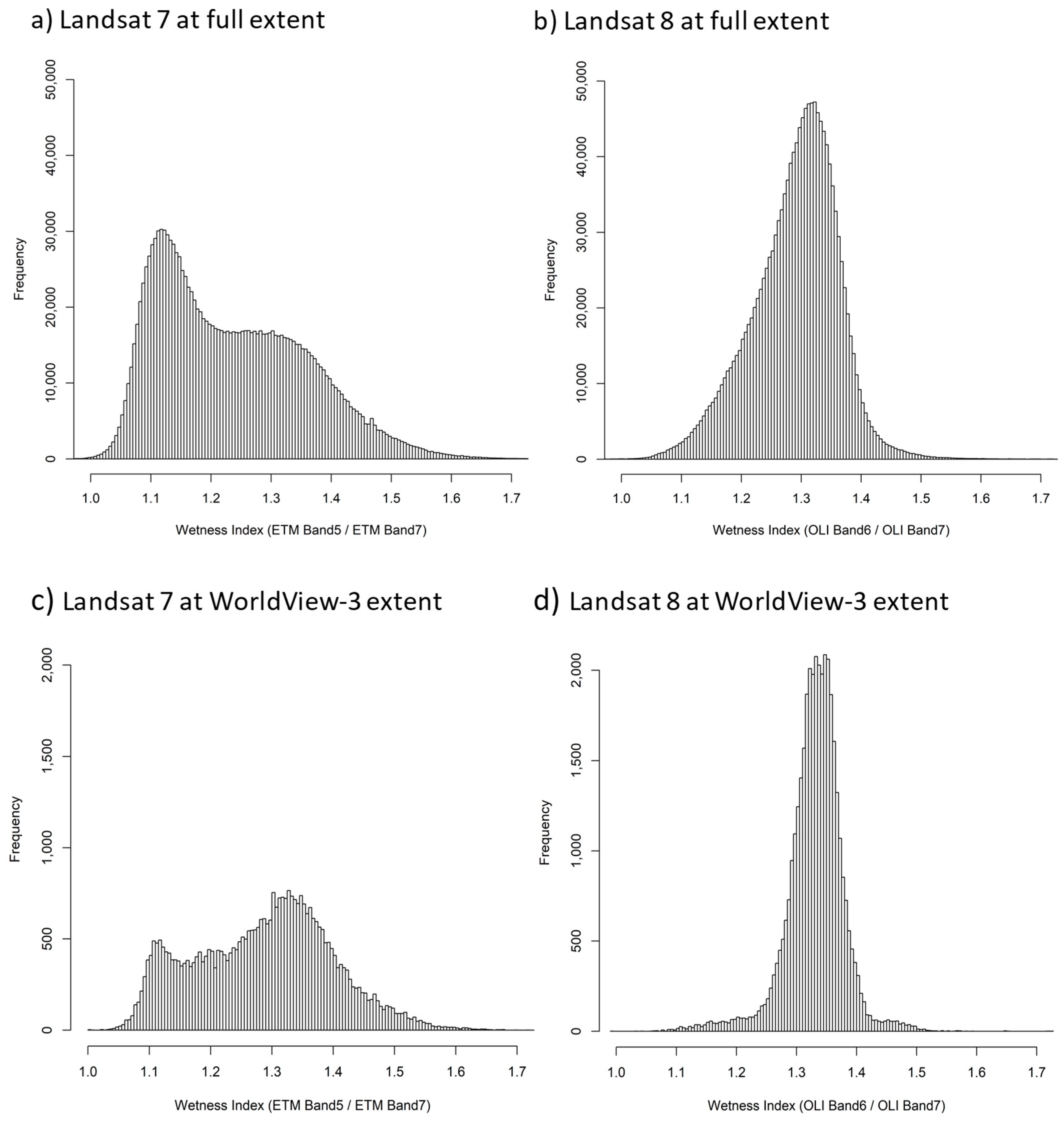
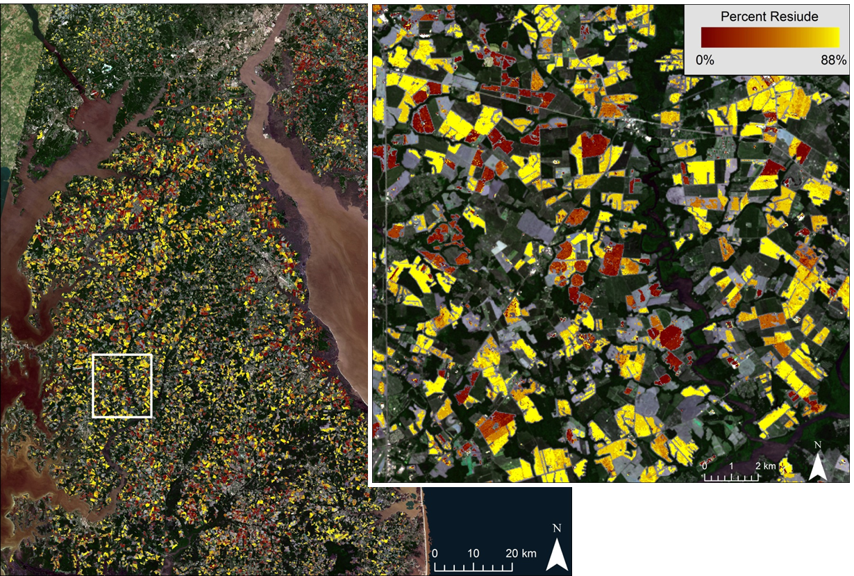
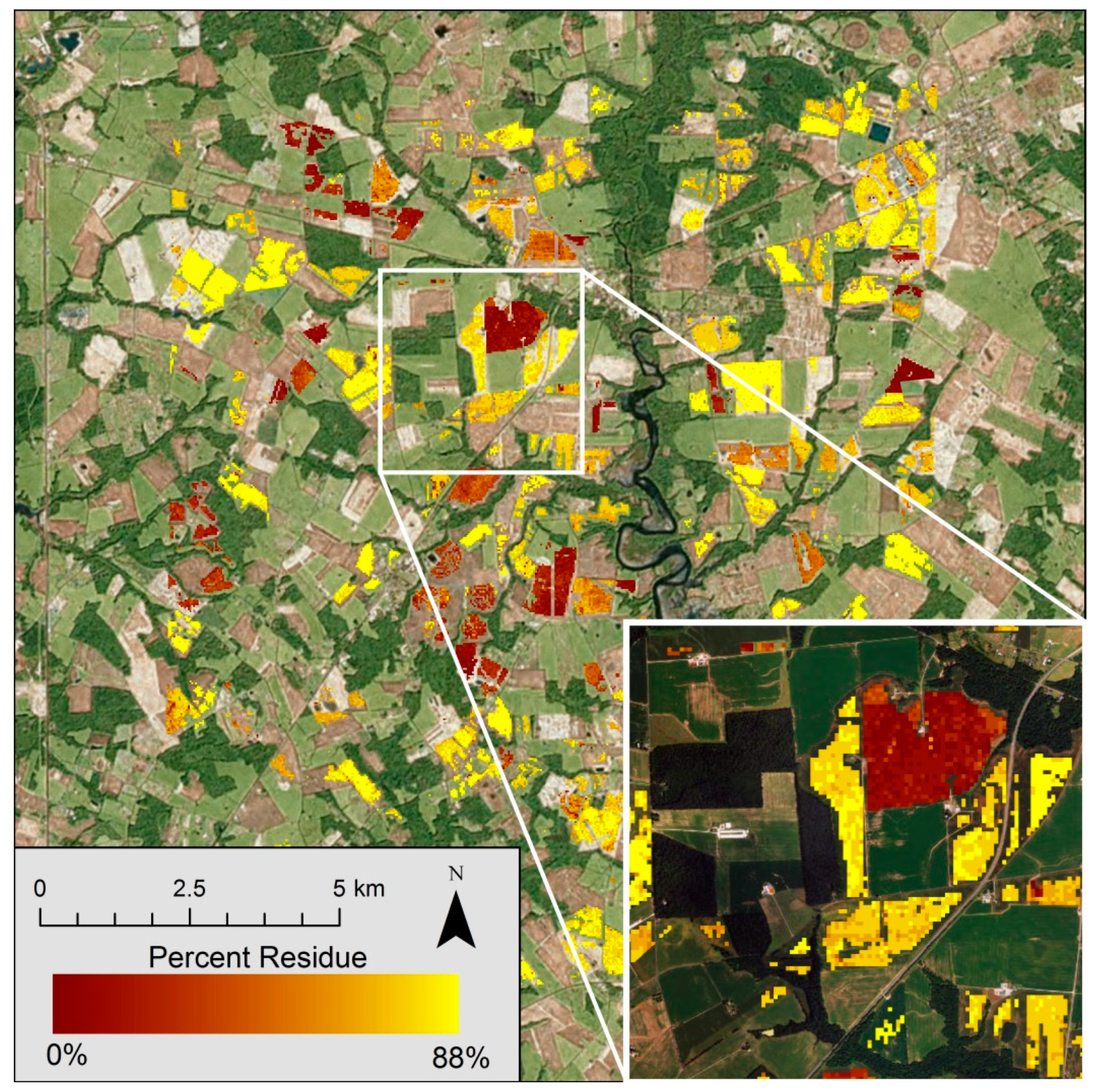
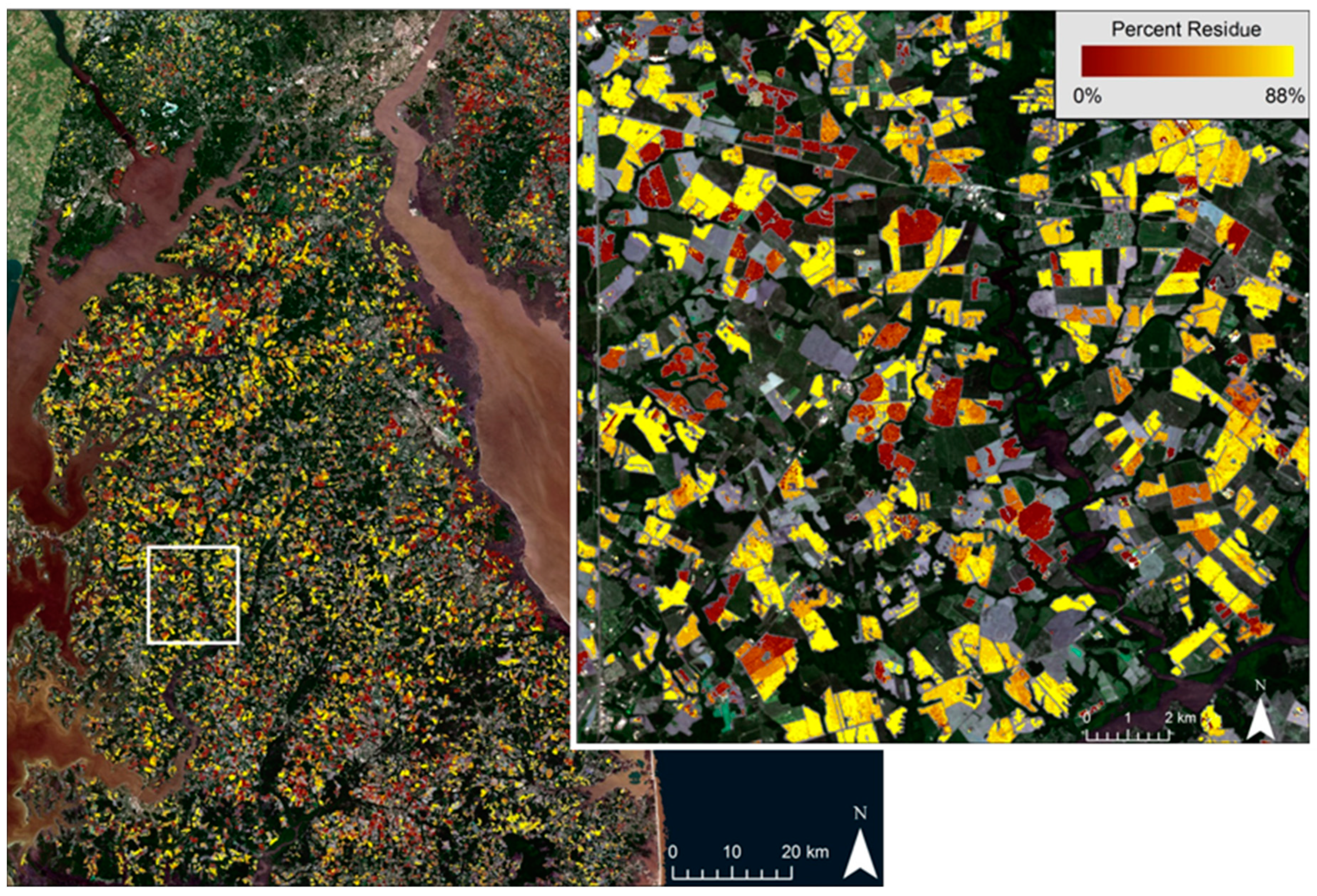
This research described a unique method that combined a small field sampling campaign, WorldView-3 (WV3) shortwave infrared (SWIR) imagery analysis, and Landsat imagery analysis to monitor crop residue conditions on the Eastern Shore of the Chesapeake Bay. Crop residue cover was successfully mapped for the entire Eastern Shore at Landsat extent and spatial resolution, with overall accuracies ranging from 92.1–93.3% (+/− 10%) using a Gradient Boosting Tree (GBT) classifier applied to a 12-band image stack of six Landsat-derived tillage indices along with reflectance values for six individual Landsat bands from the visible through the SWIR. Results were compared for two Landsat images, acquired under differing soil moisture conditions.

Overall, the GBT classifier using 12 bands (accuracy of 92.1% to 93.3%) performed better than any of the 12 bands in isolation (accuracy of 58.7% to 83.7%). The 12-band GBT classifier worked equally well for both Landsat scenes, representing different moisture conditions. However, the relative effectiveness of individual bands varied between the two Landsat scenes, which we attribute to differences in soil moisture conditions. Under dry conditions (Landsat 7) the standard broadband SWIR difference indices NDTI, STI, and mCRC (accuracy of 80.0% to 83.7%) outperformed the individual reflectance bands (accuracy of 61.6% to 74.5%), accurately detecting spectral differences in residue and soil between 1600 nm and 2200 nm. Under wet conditions (Landsat 8) this was reversed, with the individual reflectance bands (accuracy of 66.4% to 80.7%) outperforming the tillage indices (accuracy of 58.7% to 76.4%), likely due to the increased contrast between residue and soil under moist conditions being captured by the reflectance measurements within each individual SWIR band. The mCRC index alone performed relatively well under both wet and dry conditions (accuracy of 76.4% and 80.0%, respectively). When compared to the WV3 SINDRI-derived CRC map, and when compared to tillage survey data from Maryland and Delaware, the GBT classification accuracy was greatest for the low-residue tillage class (CRC < 30%) and for the high residue tillage class (CRC > 60%), and was least accurate for the 30–60% CRC conservation tillage category.

The 12-band GBT classifier, trained on WV-3 SWIR CRC map output, provided an accurate map of CRC at a regional scale and displayed resilience to changing moisture conditions. Further development of moisture calibration techniques that use wetness index information derived from each satellite image to adjust pixel reflectance for variable moisture conditions may further improve the accuracy of this CRC mapping method. Accurate and resilient techniques that use satellite remote sensing to map crop residue cover at the landscape scale can help to inform the implementation and adaptive management of conservation tillage practices, assisting farmers to reduce nutrient and sediment loss from farmland, and reducing the impact of agriculture on the aquatic environment.

References

1. Sullivan, D.G.; Schomberg, H.; Endale, D.M.; Strickland, T.C. Evaluating Techniques for Determining Tillage Regime in the Southeastern Coastal Plain and Piedmont. Agron. J. 2006, 98, 1236. [Google Scholar] [CrossRef]
2. USDA. Interim Appraisal and Analysis of Conservation Alternatives; USDA Natural Resources Conservation Service: Washington, DC, USA, 2001. Available online: https://www.nrcs.usda.gov/Internet/FSE_DOCUMENTS/nrcs143_012452.pdf (accessed on 6 August 2019).
3. Zheng, B.; Campbell, J.B.; de Beurs, K.M. Remote sensing of crop residue cover using multi-temporal Landsat imagery. Remote Sens. Environ. 2012, 117, 177–183. [Google Scholar] [CrossRef]
4. USDA. Have Conservation Compliance Incentives Reduced Soil Erosion? U.S. Department of Agriculture, Economic Research Service: Washington, DC, USA, 2004. Available online: https://www.ers.usda.gov/amber-waves/2004/june/have-conservation-compliance-incentives-reduced-soil-erosion/ (accessed on 6 August 2019).
5. Chesapeake Bay Foundation. 2016 State of the Bay. 2016. Available online: https://www.cbf.org/document-library/cbf-reports/2016-state-of-the-bay-report.pdf (accessed on 16 May 2017).
6. Moyer, D.; Blomquist, J.D. Summary of Nitrogen, Phosphorus, and Suspended-Sediment Loads and Trends Measured in Nine Chesapeake Bay Tributaries: Water Year 2015 Update; U.S. Geological Survey Data Release (USGS): Reston, VA, USA, 2016. [CrossRef]
7. Chesapeake Bay Program. Quick Reference Guide for Best Management pRactices: Nonpoint Source BMPs to Reduce Nitrogen, Phosphorus and Sediment Loads to the Chesapeake Bay and Its Local Waters; Chesapeake Bay Program Office: Annapolis, MD, USA, 2018. Available online: https://www.chesapeakebay.net/documents/BMP-Guide_Full.pdf (accessed on 16 May 2019).
8. Daughtry, C.S.T.; Doraiswamy, P.C.; Hunt, E.R.; Stern, A.J.; McMurtrey, J.E.; Prueger, J.H. Remote sensing of crop residue cover and soil tillage intensity. Soil Tillage Res. 2006, 91, 101–108. [Google Scholar] [CrossRef]
9. USDA National Agricultural Statistical Service. Maryland Tillage Practices Survey Results Released; U.S. Department of Agriculture: Washington, DC, USA, 2013.
10. Quemada, M.; Daughtry, C.S.T. Spectral indices to improve crop residue cover estimation under varying moisture conditions. Remote Sens. 2016, 8, 660. [Google Scholar] [CrossRef]
11. South, S.; Qi, J.; Lusch, D.P. Optimal classification methods for mapping agricultural tillage practices. Remote Sens. Environ. 2004, 91, 90–97. [Google Scholar] [CrossRef]
12. Sullivan, D.G.; Strickland, T.C.; Masters, M.H. Satellite mapping of conservation tillage adoption in the Little River experimental watershed, Georgia. J. Soil Water Conserv. 2008, 63, 112–119. [Google Scholar] [CrossRef]
13. Van Deventer, A.P.; Ward, A.D.; Gowda, P.H.M.; Lyon, J.G. Using thematic mapper data to identify contrasting soil plains and tillage practices. Photogramm. Eng. Remote Sens. 1997, 63, 87–93. [Google Scholar]
14. Zheng, B.; Campbell, J.B.; Serbin, G.; Galbraith, J.M. Remote sensing of crop residue and tillage practices: Present capabilities and future prospects. Soil Tillage Res. 2014, 138, 26–34. [Google Scholar] [CrossRef]
15. Bégué, A.; Arvor, D.; Bellon, B.; Betbeder, J.; de Abelleyra, D.; Ferraz, R.P.D.; Lebourgeois, V.; Lelong, C.; Simões, M.; Verón, S.R. Remote sensing and cropping practices: A review. Remote Sens. 2018, 10, 99. [Google Scholar] [CrossRef]
16. Daughtry, C.S.T.; Hunt, E.R. Mitigating the effects of soil and residue water contents on remotely sensed estimates of crop residue cover. Remote Sens. Environ. 2008, 112, 1647–1657. [Google Scholar] [CrossRef]
17. Quemada, M.; Hively, W.D.; Daughtry, C.S.T.; Lamb, B.T.; Shermeyer, J. Improved crop residue cover estimates obtained by coupling spectral indices for residue and moisture. Remote Sens. Environ. 2018, 206, 33–44. [Google Scholar] [CrossRef]
18. Beeson, P.C.; Daughtry, C.S.T.; Hunt, E.R.; Akhmedov, B.; Sadeghi, A.M.; Karlen, D.L.; Tomer, M.D. Multispectral satellite mapping of crop residue cover and tillage intensity in Iowa. J. Soil Water Conserv. 2016, 71, 385–395. [Google Scholar] [CrossRef] [Green Version]
19. Serbin, G.; Hunt, E.R.; Daughtry, C.S.T.; McCarty, G.W.; Doraiswamy, P.C. An improved ASTER index for remote sensing of crop residue. Remote Sens. 2009, 4, 971–991. [Google Scholar] [CrossRef]
20. Hively, W.D.; Lamb, B.T.; Daughtry, C.S.T.; Shermeyer, J.; Mccarty, G.W.; Quemada, M. Mapping Crop Residue and Tillage Intensity Using WorldView-3 Satellite Shortwave Infrared Residue Indices. Remote Sens. 2018, 10, 1657. [Google Scholar] [CrossRef]
21. Yue, J.; Tian, Q.; Dong, X.; Xu, K.; Zhou, C. Using Hyperspectral Crop Residue Angle Index to Estimate Maize and Winter-Wheat Residue Cover: A Laboratory Study. Remote Sens. 2019, 11, 807. [Google Scholar] [CrossRef]
22. Soil Survey Staff, Natural Resources Conservation Service. Keys to Soil Taxonomy, 12th ed.; USDA-Natural Resources Conservation Service: Washington, DC, USA, 2014.
23. Schmidt, G.; Jenkerson, C.; Masek, J.; Vermote, E.; Gao, F. Landsat Ecosystem Disturbance Adaptive Processing System (LEDAPS) Algorithm Description; U.S. Goelogical Survey Open File Report 2013-1057; USGS: Reston, VA, USA, 2013.
24. U.S. Geological Survey. Product Guide: Provisional Landsat 8 Surface Reflectance Code (LASRC) Product; USGS: Reston, VA, USA, 2016.
25. Vermote, E.; Justice, C.; Claverie, M.; Franch, B. Remote Sensing of Environment Preliminary analysis of the performance of the Landsat 8/OLI land surface re fl ectance product. Remote Sens. Environ. 2016, 185, 46–56. [Google Scholar] [CrossRef]
26. Zhu, Z.; Wang, S.; Woodcock, C.E. Improvement and expansion of the Fmask algorithm: Cloud, cloud shadow, and snow detection for Landsats 4-7, 8, and Sentinel 2 images. Remote Sens. Environ. 2015, 159, 269–277. [Google Scholar] [CrossRef]
27. Daughtry, C.S.T.; Serbin, G.; Reeves, J.B.; Doraiswamy, P.C.; Hunt, E.R. Spectral reflectance of wheat residue during decomposition and remotely sensed estimates of residue cover. Remote Sens. 2010, 2, 416–431. [Google Scholar] [CrossRef]
28. Serbin, G.; Daughtry, C.S.T.; Hunt, E.R.; Brown, D.J.; McCarty, G.W. Effect of Soil Spectral Properties on Remote Sensing of Crop Residue Cover. Soil Sci. Soc. Am. J. 2009, 73, 1545. [Google Scholar] [CrossRef]
29. McNairn, H.; Protz, R. Mapping Corn Residue Cover on Agricultural Fields in Oxford County, Ontario, Using Thematic Mapper. Can. J. Remote Sens. 1993, 19, 152–159. [Google Scholar] [CrossRef]
30. Qi, J.; Marset, R.; Heilman, P.; Biedenbender, S.; Moran, S.; Goodrich, D. RANGES Improves Satellite-based Information and Land Cover Assessments in Southwest United States. EOS Trans. Am. Geophys. Union 2002, 83. [Google Scholar] [CrossRef]
31. Richardson, A.J.; Wiegand, C.L. Distinguishing Vegetation from Soil Background Information. Photgramm. Eng. Remote Sens. 1977, 43, 1541–1552. [Google Scholar]
32. Rondeaux, G.; Steven, M.; Baret, F. Optimization of Soil-Adjusted Vegetation Indices. Remote Sens. Environ. 1996, 107, 95–107. [Google Scholar] [CrossRef]
33. Gitelson, A.A.; Stark, R.; Grits, U.; Rundquist, D.; Kaufman, Y.; Derry, D. Vegetation and soil lines in visible spectral space: A concept and technique for remote estimation of vegetation fraction. Int. J. Remote Sens. 2002, 23, 2537–2562. [Google Scholar] [CrossRef]
34. Xue, J.; Su, B. Significant Remote Sensing Vegetation Indices: A Review of Developments and Applications. J. Sens. 2017, 17. [Google Scholar] [CrossRef]
35. Daughtry, C.S.T.; Hunt, E.R.; Doraiswamy, P.C.; McMurtrey, J.E. Remote Sensing the Spatial Distribution of Crop Residues. Agron. J. 2005, 864–871. [Google Scholar] [CrossRef]
36. USDA. 2015 CropScape-Cropland Data Layer. 2015. Available online: https://nassgeodata.gmu.edu/CropScape/ (accessed on 16 May 2019).
37. Homer, B.C.; Dewitz, J.; Yang, L.; Jin, S.; Danielson, P.; Coulston, J.; Herold, N.; Wickham, J.; Megown, K. Completion of the 2011 National Land Cover Database for the Conterminous United States—Representing a Decade of Land Cover Change Information. Photogramm. Eng. Remote Sens. 2015, 81, 345–354. [Google Scholar]
38. Li, Z.; Huffman, T.; McConkey, B.; Townley-Smith, L. Monitoring and modeling spatial and temporal patterns of grassland dynamics using time-series MODIS NDVI with climate and stocking data. Remote Sens. Environ. 2013, 138, 232–244. [Google Scholar] [CrossRef]
39. Jones, J.W. Improved Automated Detection of Subpixel-Scale Inundation—Revised Dynamic Surface Water Extent (DSWE) Partial Surface Water Tests. Remote Sens. 2019, 11, 374. [Google Scholar] [CrossRef]
40. USDA. Farm Service Agency, Common Land Unit (CLU). 2019. Available online: https://www.fsa.usda.gov/programs-and-services/aerial-photography/imagery-products/common-land-unit-clu/index (accessed on 21 June 2019).
41. Friedman, J.H. Stochastic gradient boosting. Comput. Stat. Data Anal. 2002, 38, 367–378. [Google Scholar] [CrossRef]
42. Hastie, T.; Tibshirani, R.; Friedman, J. The Elements of Statistical Learning, 2nd ed.; Springer Science and Business Media: Berlin, Germany, 2002. [Google Scholar] [CrossRef]
43. Chesapeake Bay Program. Chesapeake Assessment and Scenario Tool (CAST) Version. 2017. Available online: https://cast.chesapeakebay.net/Home/SourceData (accessed on 6 August 2019).
44. DNREC. State of Delatare Nonpoint Source Best Management Practice Implementation Data Quality Assurance Project and Verification Plan; Delaware Department of Natural Resources and Environmental Control: Dover, DE, USA, 2018.
45. Coppin, P.; Jonckheere, I.; Nackaerts, K. Digital Change Detection Methods in Ecosystem Monitoring: A Review Review Article. Int. J. Remote Sens. 2004, 25. [Google Scholar] [CrossRef]
46. Shermeyer, J.; Haack, B. Remote seensing change detection methods to track deforestation and growth in threatened rainforests in Madre de Dios, Peru. J. Appl. Remote Sens. 2015, 9, 096040. [Google Scholar] [CrossRef]
47. Hively, W.D.; Lamb, B.T.; Daughtry, C.S.T.; Shermeyer, J.; McCarty, G.M. Worldview-3 Satellite Imagery and Crop Residue Field Data Collection, Talbot County, MD, May 2015; U.S. Geological Survey Data Release (USGS): Reston, VA, USA, 2015. [CrossRef]
Figure 1. Study area including the Eastern Shore of Maryland and Delaware. The Landsat footprint is outlined in red, and the WorldView-3 image and collaborating farm where the field sampling campaign occurred (zoom window) is outlined in white.
Remotesensing 11 01857 g001
Figure 2. Correlation of WorldView-3 Shortwave Infrared Normalized Difference Residue Index (SINDRI) with in-field measurements of percent residue cover. Figure modified from previous work [20].
Remotesensing 11 01857 g002
Figure 3. Map of percent residue cover derived from WorldView-3 shortwave infrared normalized difference index SINDRI (Hively et. al., 2018a) showing calculated percent residue in non-vegetated areas (normalized difference vegetation index NDVI < 0.3) with National Agriculture Imagery Program true color imagery in the remaining areas. Inset zoom depicts how crop residue outcomes track with field-specific management.
Remotesensing 11 01857 g003
Figure 4. Landsat 7 (ETM+) map of calculated percent crop residue cover on non-vegetated agricultural fields, overlaid on natural-color Landsat 7 imagery. Striping results from missing data due to Landsat 7 scan line corrector errors.
Remotesensing 11 01857 g004
Figure 5. Landsat 8 (OLI) map of calculated percent crop residue cover on non-vegetated agricultural fields, overlaid on natural-color Landsat 8 imagery.
Remotesensing 11 01857 g005
Figure 6. Comparison of Wetness Index values for Landsat 7 imagery (drier conditions) and Landsat 8 imagery (wetter conditions) at (a,b) the full extent of the Landsat footprint and (c,d) the limited extent of the Worldview-3 footprint, depicting the effect of rainfall on soil wetness (9.4 cm precipitation recorded between 14 May and 22 May).
Remotesensing 11 01857 g006
Figure 7. The mean spectral differences related to soil moisture for (a) normalized difference tillage index NDTI, (b) shortwave infrared reflectance band 2 SWIR2 (2.09–2.35 μm), and (c) modified crop residue cover index mCRC. Mean spectral responses are depicted as points; error bars depict one standard deviation from the mean.
Remotesensing 11 01857 g007