On the Segmentation of the Cephalonia–Lefkada Transform Fault Zone (Greece) from an InSAR Multi-Mode Dataset of the Lefkada 2015 Sequence

 , , ,
, , , 
Abstract
1. Introduction
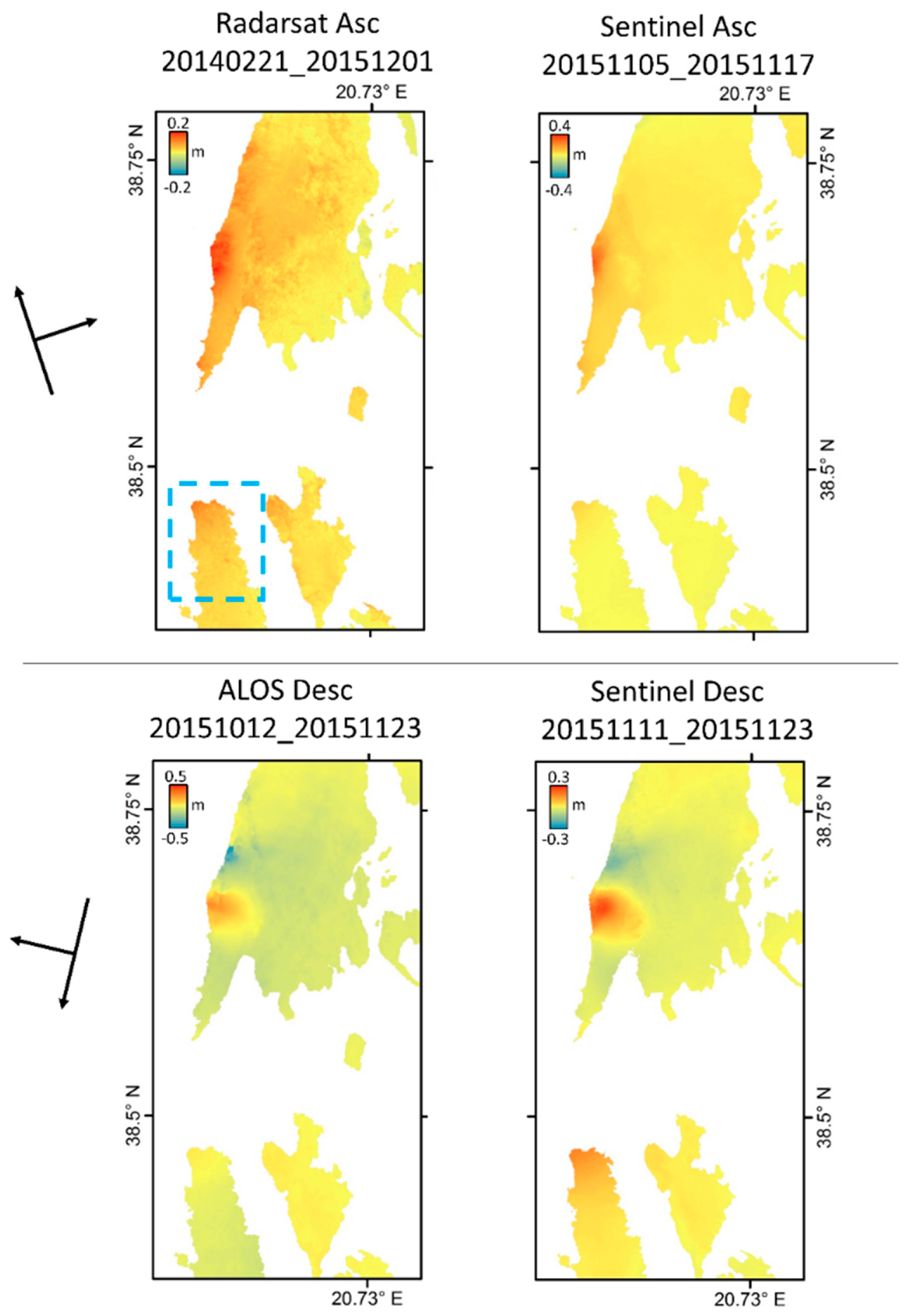
2. Data and Methods
3. Deformation and Seismic Source Modelling Results
3.1. Single Fault Model
3.2. Two-Fault Model
4. Further Interpretation of the Two-Fault Model
Stress Transfer Loading
5. Discussion and Conclusions
Supplementary Materials
Author Contributions
Funding
Acknowledgments
Conflicts of Interest
References
- Pearce, F.D.; Rondenay, S.; Sachpazi, M.; Charalampakis, M.; Royden, L.H. Seismic investigation of the transition from continental to oceanic subduction along the western Hellenic Subduction Zone. J. Geophys. Res. 2012, 117, B07306. [Google Scholar] [CrossRef]
- Papazachos, B.C.; Papazachou, C.B. The Earthquakes of Greece. 1997. Available online: http://nemertes.lis.upatras.gr/jspui/handle/10889/817 (accessed on 5 April 2019).
- Kiratzi, A.; Langston, C. Moment tensor inversion of the January 17, 1983 Kefallinia event of Ionian Islands (Greece). Geoph. Jour. Int. 1991, 105, 529–535. [Google Scholar] [CrossRef]
- Louvari, E.; Kiratzi, A.; Papazachos, B.C. The Cephalonia Transform Fault and its continuation to western Lefkada Island. Tectonophysics 1999, 308, 223–236. [Google Scholar] [CrossRef]
- Sachpazi, M.; Hirn, A.; Clément, C.; Haslinger, F.; Laigle, M.; Kissling, E.; Charvis, P.; Hello, Y.; Lépine, J.C.; Sapin, M.; et al. Western Hellenic subduction and Cephalonia Transform: Local earthquakes and plate transport and strain. Tectonophysics 2000, 319, 301–331. [Google Scholar] [CrossRef]
- Scordilis, M.; Karakaisis, F.; Karacostas, G.; Panagiotopoulos, G.; Comninakis, E.; Papazachos, C. Evidence for transform faulting in the Ionian Sea: The Cephalonia Island earthquake sequence of 1983. PAGEOPH 1985, 123, 388–397. [Google Scholar] [CrossRef]
- Avallone, A.; Cirella, A.; Cheloni, D.; Tolomei, C.; Theodoulidis, N.; Piatanesi, A.; Briole, P.; Ganas, A. Near-source high-rate GPS, strong motion and InSAR observations to image the 2015 Lefkada (Greece) Earthquake rupture history. Sci. Rep. 2017, 7, 10358. [Google Scholar] [CrossRef] [PubMed]
- Bie, L.; González, P.J.; Rietbrock, A. Slip distribution of the 2015 Lefkada earthquake and its implications for fault segmentation. Geoph. Jour. Int. 2017, 210, 420–427. [Google Scholar] [CrossRef]
- Chousianitis, K.; Konca, A.O.; Tselentis, G.A.; Papadopoulos, G.A.; Gianniou, M. Slip model of the 17 November 2015 Mw =6.5 Lefkada earthquake from the joint inversion of geodetic and seismic data. Geophys. Res. Lett. 2016, 43, 7973–7981. [Google Scholar] [CrossRef]
- Ganas, A.; Elias, P.; Bozionelos, G.; Papathanassiou, G.; Avallone, A.; Papastergios, A.; Valkaniotis, S.; Parcharidis, I.; Briole, P. Coseismic deformation, field observations and seismic fault of the 17 November 2015 M = 6.5, Lefkada Island, Greece earthquake. Tectonophysics 2016, 687, 210–222. [Google Scholar] [CrossRef]
- Melgar, D.; Ganas, A.; Geng, J.; Liang, C.; Fielding, E.J.; Kassaras, I. Source characteristics of the 2015 Mw6.5Lefkada, Greece, strike-slip earthquake. J. Geophys. Res. Solid Earth 2017, 122, 2260–2273. [Google Scholar]
- Saltogianni, V.; Taymaz, T.; Yolsal-Çevikbilen, S.; Eken, T.; Moschas, F.; Stiros, S. Fault Model for the 2015 Leucas (Aegean Arc) Earthquake: Analysis Based on Seismological and Geodetic Observations. Bull. Seismol. Soc. Am. 2017, 107. [Google Scholar] [CrossRef]
- Sokos, E.; Zahradník, J.; Gallovic, F.; Serpetsidaki, A.; Plicka, V.; Kiratzi, A. Asperity break after 12 years: The Mw6.4 2015 Lefkada (Greece) earthquake. Geophys. Res. Lett. 2016, 43. [Google Scholar] [CrossRef]
- Papathanassiou, G.; Valkaniotis, S.; Ganas, A.; Grendas, N.; Kollia, E. The November 17th, 2015 Lefkada (Greece) strike-slip earthquake: Field mapping of generated failures and assessment of macroseismic intensity ESI-07. Eng. Geol. 2015, 220, 13–30. [Google Scholar] [CrossRef]
- Lekkas, E.; Mavroulis, S.; Carydis, P.; Alexoudi, V. The 17 November 2015 Mw 6.4 Lefkas (Ionian Sea, Western Greece) Earthquake: Impact on Environment and Buildings. Geotech. Geol. Eng. 2018, 36, 2109–2142. [Google Scholar] [CrossRef]
- Lekkas, E.; Mavroulis, S.; Alexoudi, V. Field observations of the 2015 (November 17, Mw 6.4) Lefkas (Ionian sea, western Greece) earthquake impact on natural environment and building stock of Lefkas island. Bull. Geol. Soc. Greece 2016, 50, 499–510. [Google Scholar] [CrossRef][Green Version]
- Kassaras, I.; Kazantzidou-Firtinidou, D.; Ganas, A.; Tonna, S.; Pomonis, A.; Karakostas, C.; Papadatou-Giannopoulou, C.; Psarris, D.; Lekkas, E.; Makropoulos, K. On the Lefkas (Ionian Sea) November 17, 2015 Mw = 6.5 Earthquake Macroseismic Effects. J. Earthq. Eng. 2018. [Google Scholar] [CrossRef]
- Ganas, A.; Briole, P.; Melgar, D.; Bozionelos, G.; Valkaniotis, S.; Avallone, A.; Papathanassiou, G.; Mendonidis, E.; Elias, P. Coseismic Deformation and Seismic fault of the 17 November 2015 M=6.5 earthquake, Lefkada island. Bull. Geol. Soc. Greece 2016, 50, 491–498. [Google Scholar] [CrossRef]
- Sokos, E.; Kiratzi, A.; Gallovič, F.; Zahradník, J.; Serpetsidaki, A.; Plicka, V.; Janský, J.; Kostelecký, J.; Tselentis, G.A. Rupture process of the 2014 Cephalonia, Greece, earthquake doublet (Mw6) as inferred from regional and local seismic data. Tectonophysics 2015, 656, 131–141. [Google Scholar] [CrossRef]
- Kiratzi, A. Mechanisms of Earthquakes in Aegean. In Encyclopedia of Earthquake Engineering; Beer, M., Kougioumtzoglou, I.A., Patelli, E., Siu-Kui, I., Eds.; Springer: Berlin/Heidelberg, Germany, 2014; pp. 1–22. [Google Scholar]
- Papadimitriou, E.; Karakostas, V.; Mesimeri, M.; Chouliaras, G.; Kourouklas, C.H. The Mw 6.5 17 November 2015 Lefkada (Greece) Earthquake: Structural Interpretation by Means of the Aftershock Analysis. Pure Appl. Geophys. 2017, 174, 3869–3888. [Google Scholar] [CrossRef]
- Polcari, M.; Palano, M.; Fernández, J.; Samsonov, S.V.; Stramondo, S.; Zerbini, S. 3D displacement field retrieved by integrating Sentinel-1 InSAR and GPS data: The 2014 South Napa earthquake. Eur. J. Remote Sens. 2016, 49. [Google Scholar] [CrossRef]
- Polcari, M.; Albano, M.; Atzori, S.; Bignami, C.; Stramondo, S. The Causative Fault of the 2016 Mw 6.1 Petermann Ranges Intraplate Earthquake (Central Australia) Retrieved by C- and L-Band InSAR Data. Remote Sens. 2018, 10, 1311. [Google Scholar] [CrossRef]
- Barba-Sevilla, M.; Baird, B.W.; Liel, A.B.; Tiampo, K.F. Hazard Implications of the 2016 Mw 5.0 Cushing, OK Earthquake from a Joint Analysis of Damage and InSAR Data. Remote Sens. 2018, 10, 1715. [Google Scholar] [CrossRef]
- Albano, M.; Polcari, M.; Bignami, C.; Moro, M.; Saroli, M.; Stramondo, S. Did anthropogenic activities trigger the 3 April 2017, Mw 6.5 Botswana earthquake? Remote Sens. 2017, 9, 1028. [Google Scholar] [CrossRef]
- Vajedian, S.; Motagh, M.; Mousavi, Z.; Motaghi, K.; Fielding, E.J.; Akbari, B.; Wetzel, H.U.; Darabi, A. Coseismic Deformation Field of the Mw 7.3 12 November 2017 Sarpol-e Zahab (Iran) Earthquake: A Decoupling Horizon in the Northern Zagros Mountains Inferred from InSAR Observations. Remote Sens. 2018, 10, 1589. [Google Scholar] [CrossRef]
- Boncori, J.P.M.; Papoutsis, I.; Pezzo, G.; Tolomei, C.; Atzori, S.; Ganas, A.; Karastathis, V.; Salvi, S.; Kontoes, C.; Antonioli, A. The February 2014 Cephalonia earthquake (Greece): 3D deformation field and source modeling from multiple SAR techniques. Seism. Res. Lett. 2015, 86, 124–137. [Google Scholar] [CrossRef]
- Massonnet, D.; Feigl, K.L. Satellite radar interferometric map of the coseismic deformation field of the M = 6.1 Eureka Valley, California earthquake of May 17, 1993. Geophys. Res. Lett. 1995, 22, 1541–1544. [Google Scholar] [CrossRef]
- Farr, T.G.; Kobrick, M. Shuttle radar topography mission produces a wealth of data. Eos Trans. 2000, 81, 583–585. [Google Scholar] [CrossRef]
- Goldstein, R.; Werner, C. Radar Interferogram filtering for geophysical applications Radar interferogram filtering for geophysical applications. Geophys. Res. Lett. 1998, 25, 4035–4038. [Google Scholar] [CrossRef]
- Costantini, M. A novel phase unwrapping method based on network programming. Geosci. Remote Sens. 1998, 36, 813–821. [Google Scholar] [CrossRef]
- Okada, Y. Surface deformation due to shear and tensile faults in a half-space. Bull. Seism. Soc. Am. 1985, 75, 1135–1154. [Google Scholar]
- Levenberg, K. A method for the solution of certain problems in least squares. Q. Appl. Math. 1944, 2, 164–168. [Google Scholar] [CrossRef]
- Marquardt, D. An Algorithm for Least-Squares Estimation of Nonlinear Parameters. SIAM J. Appl. Math. 1963, 11, 431–441. [Google Scholar] [CrossRef]
- Atzori, S.; Hunstad, I.; Chini, M.; Salvi, S.; Tolomei, C.; Bignami, C.; Stramondo, S.; Trasatti, E.; Antonioli, A.; Boschi, E. Finite fault inversion of DInSAR coseismic displacement of the 2009 L’Aquila earthquake (central Italy). Geophys. Res. Lett. 2009, 36, L15305. [Google Scholar] [CrossRef]
- Menke, W. Geophysical Data Analysis: Discrete Inverse Theory; Academic Press: San Diego, CA, USA, 1989. [Google Scholar]
- Elliott, J.R.; Walters, R.J.; Wright, T.J. The role of space-based observation in understanding and responding to active tectonics and earthquakes. Nat. Commun. 2016, 7. [Google Scholar] [CrossRef] [PubMed]
- Topographic Data. Available online: http://www.emodnet-bathymetry.eu (accessed on 5 April 2019).
- Kazantzidou-Firtinidou, D.; Kassaras, I.; Tonna, S.; Ganas, A.; Vintzileou, E.; Chesi, C. Τhe November 2015 Mw6.4 earthquake effects in Lefkas Island. In Proceedings of the 1st International Conference on Natural Hazards Infrastructure, Chania, Greece, 18–21 June 2016. [Google Scholar]
- Atzori, S.; Antonioli, A. Optimal fault resolution in geodetic inversion of coseismic data. Geophys. J. Int. 2011, 185, 529–538. [Google Scholar] [CrossRef]
- Harris, R.; Simpson, R.W. Suppression of large earthquakes by stress shadows: A comparison of Coulomb and rate-and-state failure. J. Geophys. Res. 1998, 103, 24439–24451. [Google Scholar] [CrossRef]
- Papadimitriou, E.E. Mode of strong earthquake recurrence in central Ionian Islands (Greece). Possible triggering due to Coulomb stress changes generated by the occurrence of previous strong shocks. Bull. Seism. Soc. Am. 2002, 92, 3293–3308. [Google Scholar] [CrossRef]
- Stiros, S.; Pirazzoli, P.; Labore, J.; Laborel-Deguen, F. The 1953 earthquake in Cephalonia (Western Hellenic Arc): Coastal uplift and halotectonic faulting. Geophys. J. Int. 1994, 117, 834–849. [Google Scholar] [CrossRef]
- Karakitsios, V.; Rigakis, N. Evolution and Petroleum potential of western Greece. J. Pet. Geolo. 2007, 30, 197–218. [Google Scholar] [CrossRef]
- Saltogianni, V.; Moschas, F.; Stiros, S. The 2014 Cephalonia Earthquakes: Finite Fault Modeling, Fault Segmentation, Shear and Thrusting at the NW Aegean Arc (Greece). Pure Appl. Geophys. 2018, 175, 4145. [Google Scholar] [CrossRef]
- Brooks, M.; Ferentinos, G. Tectonics and sedimentation in the Gulf of Corinth and the Zakynthos and Kefallinia channels, Western Greece. Tectonophysics 1984, 101, 25–54. [Google Scholar] [CrossRef]
- Velaj, T.; Davison, I.; Serjani, A.; Alsop, I. Thrust tectonics and the role of evaporites in the Ionian Zone of the Albanides. AAPG Bull. 1999, 83, 1408–1425. [Google Scholar]
- Scuderi, M.M.; Niemeijer, A.R.; Collettini, C.; Marone, C. Frictional properties and slip stability of active faults within carbonate–evaporite sequences: The role of dolomite and anhydrite. Earth Planet. Sci. Lett. 2013. [Google Scholar] [CrossRef]


| Satellite | Master Date (m/d/y) | Slave Date (m/d/y) | Temporal Baseline (days) | Normal Baseline (m) | Pass | Linear Inversion RMS (m) |
|---|---|---|---|---|---|---|
| Radarsat-2 | 2/21/2014 | 12/1/2015 | 648 | 165.4 | Ascending | 0.016 |
| Sentinel-1 | 11/5/2015 | 11/17/2015 | 12 | 22.5 | Ascending | 0.018 |
| ALOS-2 | 10/12/2015 | 11/23/2015 | 42 | 77.35 | Descending | 0.025 |
| Sentinel-1 | 11/11/2015 | 11/23/2015 | 12 | 66.2 | Descending | 0.012 |
| Segment F1 | |||||
| Strike° | Dip° | Rake° | Length (km) | Width (km) | Max Slip (m) |
| 13 | 70 | 158 | 32 | 10 | 2.9 |
| Segment F2 | |||||
| Strike° | Dip° | Rake° | Length (km) | Width (km) | Max Slip (m) |
| 43 | 90 | 108 | 25 | 10 | 1.6 |
© 2019 by the authors. Licensee MDPI, Basel, Switzerland. This article is an open access article distributed under the terms and conditions of the Creative Commons Attribution (CC BY) license (http://creativecommons.org/licenses/by/4.0/).
Share and Cite
Svigkas, N.; Atzori, S.; Kiratzi, A.; Tolomei, C.; Antonioli, A.; Papoutsis, I.; Salvi, S.; Kontoes, C. On the Segmentation of the Cephalonia–Lefkada Transform Fault Zone (Greece) from an InSAR Multi-Mode Dataset of the Lefkada 2015 Sequence. Remote Sens. 2019, 11, 1848. https://doi.org/10.3390/rs11161848
Svigkas N, Atzori S, Kiratzi A, Tolomei C, Antonioli A, Papoutsis I, Salvi S, Kontoes C. On the Segmentation of the Cephalonia–Lefkada Transform Fault Zone (Greece) from an InSAR Multi-Mode Dataset of the Lefkada 2015 Sequence. Remote Sensing. 2019; 11(16):1848. https://doi.org/10.3390/rs11161848
Chicago/Turabian StyleSvigkas, Nikos, Simone Atzori, Anastasia Kiratzi, Cristiano Tolomei, Andrea Antonioli, Ioannis Papoutsis, Stefano Salvi, and Charalampos (Haris) Kontoes. 2019. "On the Segmentation of the Cephalonia–Lefkada Transform Fault Zone (Greece) from an InSAR Multi-Mode Dataset of the Lefkada 2015 Sequence" Remote Sensing 11, no. 16: 1848. https://doi.org/10.3390/rs11161848
APA StyleSvigkas, N., Atzori, S., Kiratzi, A., Tolomei, C., Antonioli, A., Papoutsis, I., Salvi, S., & Kontoes, C. (2019). On the Segmentation of the Cephalonia–Lefkada Transform Fault Zone (Greece) from an InSAR Multi-Mode Dataset of the Lefkada 2015 Sequence. Remote Sensing, 11(16), 1848. https://doi.org/10.3390/rs11161848