Improving the Accuracy of Regional Ionospheric Mapping with Double-Difference Carrier Phase Measurement

Abstract

Regional augmentation systems for a global navigation satellite system (GNSS) provide an ionospheric map correction to the user in order to remove the ionospheric delay error. Measurements are collected from multiple reference stations to estimate the ionospheric map. During this process, the pseudorange measurement error of a reference station causes an error in the correction, which is more evident at edge areas and causes a large error for low-elevation satellites. In this study, an ionospheric modeling algorithm was developed that uses the carrier phase with the pseudorange to greatly reduce the error. The integer-resolved double-difference carrier phase can be obtained through ambiguity resolution method, and the measurement is directly utilized in ionospheric modeling. The performance of the developed method was tested in simulations and with real data for validation. The results of users at various locations showed that the method effectively improved the accuracy of the correction.

1. Introduction

Ionospheric delay is a major source of error for localization systems based on a global navigation satellite system (GNSS). Multi-frequency receivers can remove ionospheric delay by using the dispersive properties of the ionosphere. Recently, a low-cost, dual-frequency receiver has been developed. However, most low-cost GNSS receivers can receive only a single frequency signal and cannot remove the ionospheric error by themselves. GPS satellites broadcast the parameters of the Klobuchar ionospheric model [1]. Users can compensate for the ionospheric error by using the broadcasted parameter; however, this usually removes only 50% of the total delay. For more precise navigation, an augmentation system is needed.

For a code-based augmentation system, undifferenced ionospheric delay correction is necessary to remove the ionospheric delay error. Local area differential GNSS (LADGNSS) provides a pseudorange correction that is the sum of the signal-in-space (SIS) error and propagation error [2]. It is effective when the user is near a reference station. However, if the user is several hundred kilometers away from the reference station, the residual error after the correction increases because of the spatial decorrelation property of the error sources. To overcome this problem, wide-area differential GNSSs such as satellite-based augmentation systems (SBASs) correct each error in vector quantities [3]. Because the correction is provided in vectors, users can apply the appropriate pseudorange correction according to their position. For the ionospheric error, a 2D ionospheric map is provided to the user. Ionospheric correction is also important for carrier phase-based augmentation systems, such as real-time kinematics (RTK). Like in code-based augmentation systems, standard RTK performance is degraded as the baseline length becomes larger. Network RTK was developed to overcome this limitation. After ambiguities among reference stations are fixed, error corrections are estimated and transmitted to users. For ionospheric delay error, one of the most effective methods is providing double-difference ionospheric corrections by interpolating those obtained from reference stations [4,5,6]. A predictive regional ionosphere model was also proposed and investigated for ionospheric correction [7].

In this study, we focus on generating accurate ionospheric correction in the form of a 2D ionosphere map. To generate the correction data, multiple reference stations were distributed over the service area. Dual-frequency measurements were collected from multiple reference stations and GNSS satellites to obtain the ionospheric delay at various locations. If the ionosphere is assumed to be a thin shell, the measured slant ionospheric delay is converted to a vertical delay [8]. Then, a 2D ionospheric map can be constructed with a specific model.

Several reasons limit the accuracy of the ionospheric map correction. First, the thin-shell approach cannot perfectly emulate the real world [9]. In addition, the modeling resolution can affect the performance. When an ionospheric storm occurs, the ionosphere shows very high dynamic temporal and spatial variations, which aggravates the above limitations [10]. Another limitation is the measurement error of the reference station, which was the main focus of this study.

When the ionospheric map is estimated for an augmentation system, the ionospheric delay is usually measured according to the pseudorange. The absolute ionospheric delay of each signal path can be acquired with the pseudorange. While this measurement provides the advantage of being easy to use for ionospheric modeling, the error can be a problem. Because the pseudorange has a relatively high measurement error owing to the noise and multipath effect, an estimation error occurs in the ionospheric map. Reference stations try to mitigate this error by using a multipath-mitigation antenna or tracking loop [11]. Despite this effort, the pseudorange measurement error can be on the order of meters. There can be severe measurement errors, especially when a satellite has low elevation angle [12]. Because of the large measurement error at low elevations, the edges of the estimated ionospheric map have degraded results compared with the central area.

To overcome the correction error caused by the pseudorange measurement, an ionospheric mapping algorithm was developed in this study that uses both the pseudorange and double-difference carrier phase for the regional augmentation system. Because the carrier phase has integer ambiguity, it is difficult to use directly. The ambiguity resolution technique can be used to measure the integer-resolved double difference for ionospheric modeling [13,14]. The much smaller error of the carrier phase measurement is exploited to combine the pseudorange and double-difference carrier phase. By properly weighting each measurement, the ionospheric map can be estimated with improved modeling results at the edge areas. The performance of the proposed algorithm was verified through simulations and tests with real data.

The remainder of this paper is organized as follows. Section 2 introduces the main concepts of this study through simple diagrams. Section 3 describes the details of the ionospheric modeling procedure. Section 4 presents the results of the simulation and tests with real data. Section 5 concludes the paper.

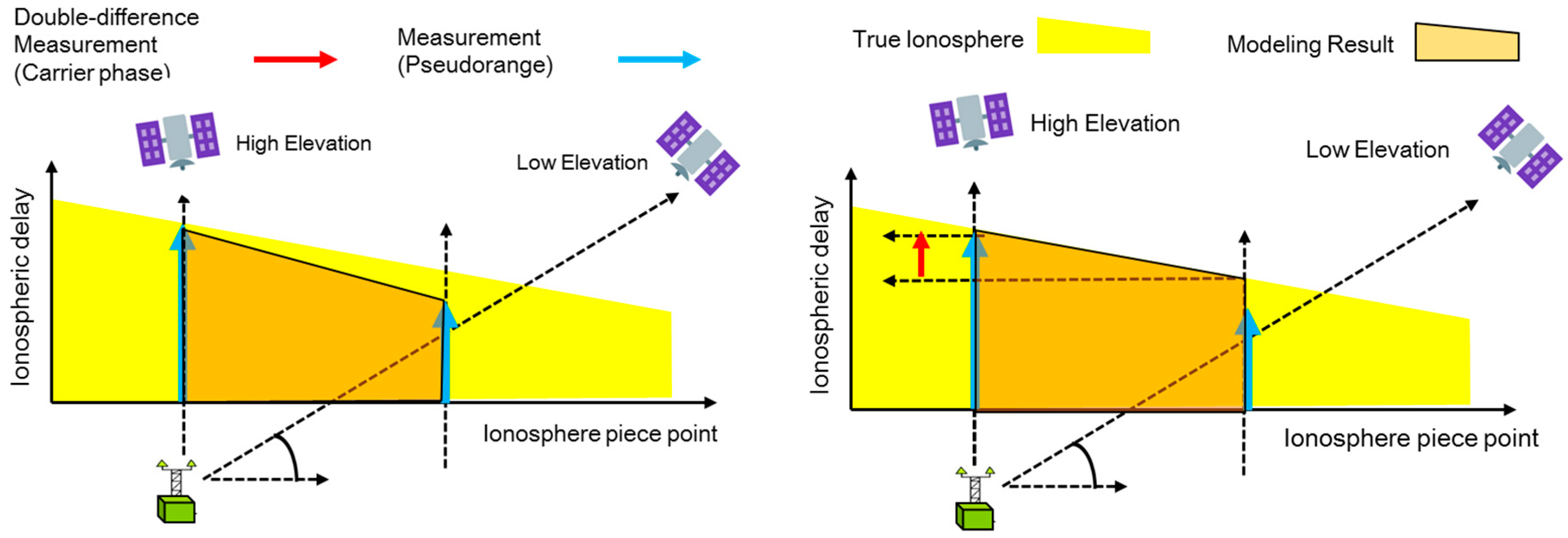
2. Benefits of the Double-Difference Carrier Phase for Ionospheric Modeling

This study focused on regional GNSS ionospheric correction. If the ionosphere is assumed to be a thin shell, a vertical ionospheric delay map can be estimated over the service area. Measurements at various ionospheric pierce points (IPPs) are collected from multiple reference stations and satellites. The main idea is to directly utilize both the pseudorange and precise difference measurements in ionospheric modeling. This section briefly introduces the difference in the results when different measurements are used. Figure 1 and Figure 2 show conceptual diagrams of the ionospheric modeling when the pseudorange and carrier phase are used. The x-axis is the IPP of each measurement. For simplicity, the ionosphere is represented in the shape of a trapezoid. The yellow and orange colors indicate the true ionosphere and modeling results, respectively.

Figure 1a shows an example of ionospheric modeling using only the pseudorange. The vertical ionospheric delay obtained from the pseudorange is denoted with blue arrows. The pseudorange has a measurement error of meters that depends on the satellite elevation angle; the measurements collected from a high-elevation satellite have a small error, while the measurements from a low-elevation satellite have a large error. When the regional ionosphere is modeled with GNSS reference stations, most measurements are obtained from high-elevation satellites at the center of the coverage. This improves the modeling accuracy at the center. At the edge of the coverage, the measurement quality is not good because the data are collected from low elevation angles. This makes the modeling results at the edges less accurate than those inside.

The carrier phase has a much smaller measurement error than the pseudorange, but it has integer ambiguity that makes it difficult to use directly. A simple way to use carrier phase is a smoothing filter [15]. Even though it has an unknown bias because of the integer ambiguity, the bias is constant over time. The rate of change in the range can be obtained precisely with the carrier phase, which can be utilized in the smoothing filter. The pseudorange measurement error can be mitigated with a smoothing filter; however, there is still a large error at the beginning of filtering. Thus, the filtered measurement also has large errors when the satellite has a low elevation angle. Because the user is located in an area with reference stations, the geometric relation between the user and each satellite is similar to those of the reference stations. The satellite elevation angle is similar for the reference stations and user. Thus, if a correction message is generated with only the pseudorange, the accuracy of the ionospheric correction for low-elevation satellites is degraded.

Unlike with the pseudorange, it is difficult to obtain the undifferenced ionospheric delay with the carrier phase. However, the integer ambiguity can be determined in the double-difference domain with ambiguity resolution methods to obtain the ambiguity-resolved double-difference ionospheric delay [13]. The characteristics of each measurement are clearly different. The pseudorange can be used to measure the undifferenced ionospheric delay, but the error is large. The double-difference carrier phase has a much smaller error but has only differenced information. In this study, the pseudorange and double-difference carrier phase were combined to take advantage of each measurement. Figure 1b shows the ionospheric modeling result with the pseudorange and double-difference carrier phase. The double-difference carrier phase-based ionospheric delay is denoted with the red arrow. Even though the pseudorange-based measurement has a large error, its characteristics are well-known. This allows each measurement to be weighted appropriately. The double-difference carrier phase can be used to precisely measure the difference in ionospheric delay at different IPPs. Based on these properties, by giving a higher weight to measurements at higher elevation angles and applying precise difference information, the accuracy of the correction at the edge areas can be improved. This alleviates the performance degradation of the correction for satellites with low elevation angles.

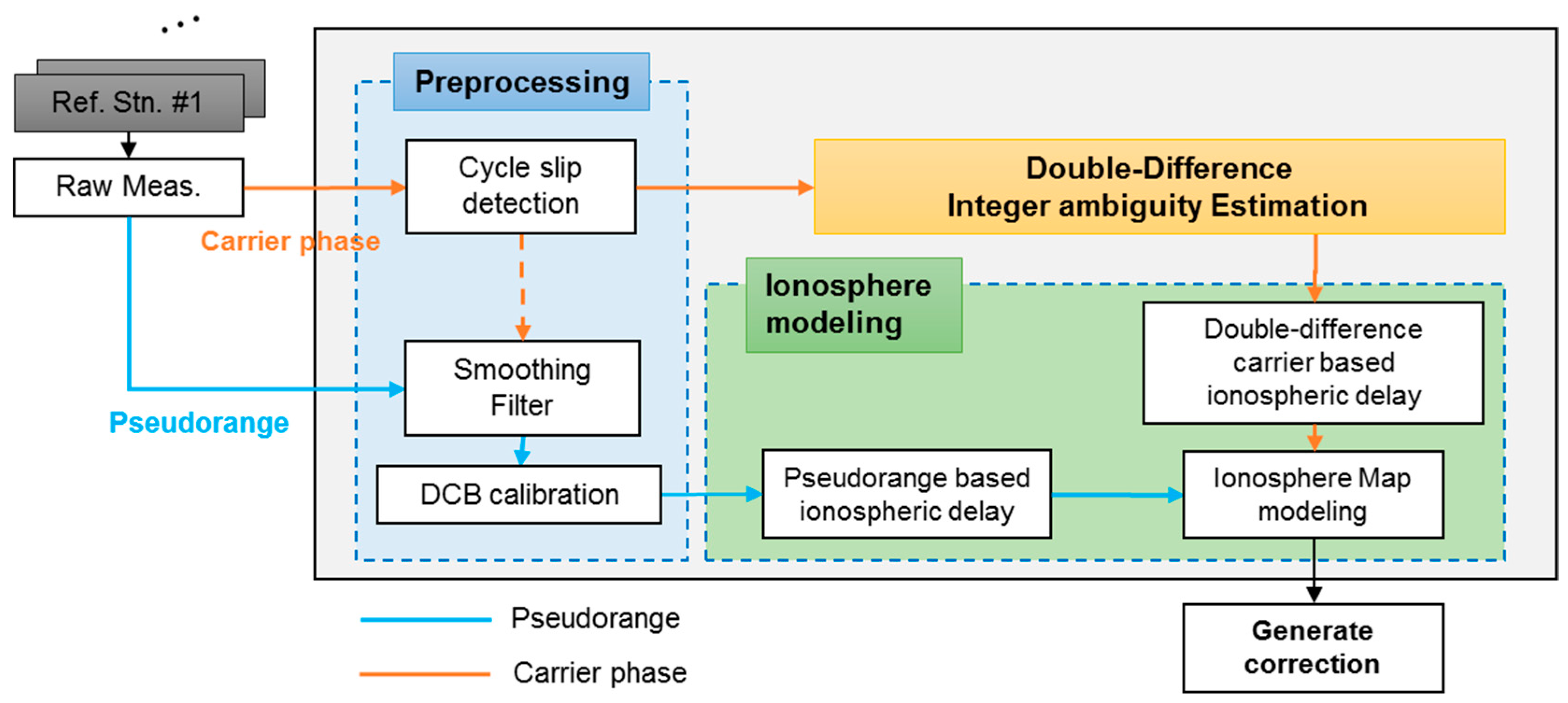
3. Ionosphere Modeling Algorithm

Figure 2 shows the overall procedure of the proposed method. Raw GNSS measurements are collected from multiple reference stations. During the preprocessing stage, cycle slip detection is carried out to prevent an unexpected jump in the carrier phase measurement. The cycle slip can be detected by monitoring the acceleration of the ionospheric delay because it is less than 10⁻⁴ $\mathrm{m}/s^2$ [16,17,18]. Unexpected outliers are detected by using the second derivative of the geometry-free combination of the carrier phase as a monitoring value. A smoothing filter and differential code bias (DCB) calibration are needed to mitigate the pseudorange measurement error. A divergence-free hatch filter is implemented to address noise and the multipath effect [16,19]. It is a type of smoothing filter that utilizes dual-frequency carrier phase measurement to remove the divergence between the pseudorange and the carrier. When the ionospheric delay is measured with the pseudorange, the DCB can be a large error source [20]. The hardware delay of the GNSS satellite and receiver have different values depending on the signal frequency. The difference in hardware delays of the pseudorange measurement obtained from two different frequencies is called the DCB; it can be several tens of nanoseconds, and should be removed. The DCBs can be estimated using a geometry-free combination of the pseudorange measurement. The geometry combination of the pseudorange comprises the ionospheric delay, satellite DCB, and receiver DCB. Because the variation of DCBs is usually very small [21], it can be assumed to be constant for a day. With a specific model for vertical ionosphere, vertical ionosphere and DCBs can be estimated simultaneously. In this study, a spherical harmonics model was adopted for the ionospheric model [21,22]. Using the measurements collected in one day, DCBs were estimated with the batch process.

The double-difference carrier phase is measured by pairing two reference stations. Among the stations, one station was selected as the master and the others were selected as auxiliaries. By pairing the master and each auxiliary, integer ambiguities were estimated. Because the surveyed position of reference stations was known, only integer ambiguities were estimated. To prevent the distance between stations from becoming too large, the reference station located at the center was selected as the master. Wide lane ambiguity was resolved by the Melbourne–Wubbena combination. Then, both ambiguities of L1 and L2 frequency were estimated using the iono-free combination [23]. Based on these, the double-difference ionospheric delay of each pair could be obtained.

The pseudorange-based measurement and ambiguity-resolved carrier phase measurement were input into the ionospheric model. The final goal of this process is to generate a vertical ionospheric delay map. Each measurement was represented by a vertical ionosphere model, which is a spherical harmonics model. Because the pseudorange measurement has a slant delay, it can be represented by multiplying the mapping function to the vertical model. The double-difference carrier phase is a linear combination of four different slant delays. It can be represented by converting the vertical model to a slant model and taking the double-difference combination of the slant model. The vertical ionospheric map is generated using both the pseudorange and double-difference carrier phase measurements from all reference stations.

Section 3.1 and Section 3.2 describe the basic GPS measurement and ionospheric model, respectively. Section 3.3 presents the observation equation for estimating the modeling parameters.

3.1. Measurement

In this study, the L1 and L2 frequencies of the Global Positioning System were measured. Equations (1)–(4) represent the raw pseudorange and carrier phase measurement [24]:

$${\rho }_1=d-(b+b_{\rho 1}^{Tx})+I+T+(B+b_{\rho 1}^{Rx})+{\epsilon }_{\rho 1}$$

(1)

$${\rho }_2=d-(b+b_{\rho 2}^{Tx})+\gamma I+T+(B+b_{\rho 2}^{Rx})+{\epsilon }_{\rho 2}$$

(2)

$${\varphi }_1=d-(b+b_{\varphi 1}^{Tx})-I+T+(B+b_{\varphi 1}^{Rx})+N_1{\lambda }_1+{\epsilon }_{\varphi 1}$$

(3)

$${\varphi }_2=d-(b+b_{\varphi 2}^{Tx})-\gamma I+T+(B+b_{\varphi 2}^{Rx})+N_2{\lambda }_2+{\epsilon }_{\varphi 2}$$

(4)

where $\rho$ is the pseudorange, $\varphi$ is the carrier phase, $d$ is the geometric distance, $I$ is the ionospheric delay for the L1 frequency, $\gamma$ is the ratio between the squares of the signal frequencies, $T$ is the tropospheric delay, b is the satellite clock bias, $B$ is the receiver clock bias, $b^{Tx}$ is the satellite hardware delay, $b^{Rx}$ is the receiver hardware delay, $\epsilon$ is the noise and multipath error, $N$ is the integer ambiguity, and $\lambda$ is the wavelength. Subscripts 1 and 2 indicate the L1 and L2 frequencies, respectively.

Because the ionosphere has a dispersive property, the L1 and L2 frequencies have different ionospheric delays. Based on this property, the ionospheric delay can be obtained by geometry-free combination. The ionospheric delay of the L1 frequency is calculated as follows:

$$\begin{array}{ll}\hfill I_{\rho ,DCB}& =\frac{{\rho }_2-{\rho }_1}{\gamma -1}\hfill \\ \hfill & =I-\frac{1}{\gamma -1}\left\{\left(b_{\rho 2}^{Tx}-b_{\rho 1}^{Tx}\right)-\left(b_{\rho 2}^{Rx}-b_{\rho 1}^{Rx}\right)+{\epsilon }_{\rho 2}-{\epsilon }_{\rho 1}\right\}\hfill \\ \hfill & =I-\frac{1}{\gamma -1}\left\{DC{B}_{\rho 1/\rho 2}^{Tx}-DC{B}_{\rho 1/\rho 2}^{Rx}\right\}+{\epsilon }_{I_{\rho }}\hfill \end{array}$$

(5)

where $I_{\rho ,DCB}$ is the pseudorange-based ionospheric delay measurement with DCBs, $I$ is the true ionospheric delay, $DC{B}_{\rho 1/\rho 2}^{Tx}$ and $DC{B}_{\rho 1/\rho 2}^{Rx}$ are the satellite DCB and receiver DCB, respectively, and ${\epsilon }_{I_{\rho }}$ is the measurement noise. After the DCBs are estimated and removed, the measurement used for ionospheric modeling is represented as follows:

$$I_{\rho }=I+{\epsilon }_{I_{\rho }}+{\epsilon }_{b^{Tx}}+{\epsilon }_{b^{Rx}}$$

(6)

where ${\epsilon }_{b^{Tx}}$ and ${\epsilon }_{b^{Rx}}$ are the estimation errors of the satellite and receiver DCBs, respectively.

The carrier phase-based ionospheric measurement is represented as follows:

$$\begin{array}{ll}{I}_{{\varphi }_{}}& =\frac{{\varphi }_1-{\varphi }_2}{\gamma -1}\\ & =I+\frac{1}{\gamma -1}\left\{-\left(b_{\varphi 1}^{Tx}-b_{\varphi 2}^{Tx}\right)+\left(b_{\varphi 1}^{Rx}-b_{\varphi 2}^{Rx}\right)+\left(N_1{\lambda }_1-N_2{\lambda }_2\right)+\left({\epsilon }_{{\varphi }_1}-{\epsilon }_{{\varphi }_2}\right)\right\}\end{array}$$

(7)

This is similar to Equation (5) except for the integer ambiguity term. The double difference of this measurement is expressed by Equation (8). During the double differencing process, both the satellite and receiver hardware delays are removed.

$$\nabla \Delta I_{\varphi ,N}=\nabla \Delta I+\frac{1}{\gamma -1}\left[\nabla \Delta \left(N_1{\lambda }_1-N_2{\lambda }_2\right)+\nabla \Delta \left({\epsilon }_{{\varphi }_1}-{\epsilon }_{{\varphi }_2}\right)\right]$$

(8)

where $\nabla \Delta I_{\varphi ,N}$ is the double-difference ionospheric delay measurement with integer ambiguity. If ambiguities are fixed correctly, the ambiguity-resolved measurement is expressed as follows:

$$\begin{array}{ll}\nabla \Delta I_{\varphi }& =\nabla \Delta I+\frac{1}{\gamma -1}\left[\nabla \Delta \left({\epsilon }_{{\varphi }_1}-{\epsilon }_{{\varphi }_2}\right)\right]\\ & =\nabla \Delta I+{\epsilon }_{\nabla \Delta I}\end{array}$$

(9)

where $\nabla \Delta I_{\varphi }$ is the ambiguity-resolved double-difference ionospheric delay measurement and ${\epsilon }_{\nabla \Delta I}$ is the measurement error.

3.2. Ionospheric Model

The thin-shell assumption was adopted for the ionospheric modeling. The slant ionospheric delay can be converted to the vertical ionospheric delay by using a simple function called the obliquity factor [8]:

$$I_S=I_V\cdot Q$$

(10)

where $I_S$ is the slant ionospheric delay, $I_V$ is the vertical ionospheric delay, and $Q$ is the obliquity factor.

Various methods have been developed for ionospheric modeling. Grid-based interpolation algorithms are a well-known example, which include the inverse distance weight (IDW) method, planar fit method, and kriging method [25,26,27,28]. These methods have different ways of calculating weights for each measurement. The IDW calculates simple weight depending on the distance. Kriging uses the statistical model to determine the weight of each measurement. Although they have differences, the basic principle is the same: they estimate the ionospheric delay at each grid point by interpolating the measurements within a certain distance limit from the grid point [26,27]. Including the double-difference measurement in grid-based algorithms is difficult because the double-difference measurement comprises four different measurements at four different locations, and there are many cases where all four different measurements are not within a certain distance limit.

Spherical harmonics was selected as the modeling method in this study [28,29]. This model represents spatial data by the linear combination of the basis functions. Distributed measurements are used to estimate the whole region at once. Spherical harmonics is suitable for double-difference measurements.

First, the spherical harmonics for the vertical ionospheric delay is expressed as follows:

$$\begin{array}{l}{I}_V(\theta ,\lambda )={\displaystyle \sum _{n=0}^N{\displaystyle \sum _{m=0}^n{P}_{nm}(\sin (\theta ))\cdot \cos (m\lambda )}}\cdot C_{nm}\\ +{\displaystyle \sum _{n=0}^N{\displaystyle \sum _{m=0}^n{P}_{nm}(\sin (\theta ))\cdot \sin (m\lambda )}}\cdot S_{nm}\end{array}$$

(11)

where $I_V$ is the vertical ionospheric delay, $\theta$ is the latitude of the IPP, $\lambda$ is the longitude of the IPP, $P_{nm}$ is the associated Legendre function, $C_{nm}$ and $S_{nm}$ are spherical harmonics coefficients, and $N$ is the degree. Measurements collected from various locations are used to estimate the coefficients. With the spherical harmonics model, the pseudorange-based slant delay measurement is represented as follows:

$$\begin{array}{ll}{I}_{\rho }& =I_V(\theta ,\lambda )\cdot Q\\ & ={\displaystyle \sum _{n=0}^N{\displaystyle \sum _{m=0}^n{P}_{nm}(\sin (\theta ))\cdot \cos (m\lambda )\cdot Q}}\cdot C_{nm}\\ & +{\displaystyle \sum _{n=0}^N{\displaystyle \sum _{m=0}^n{P}_{nm}(\sin (\theta ))\cdot \sin (m\lambda )\cdot Q}}\cdot S_{nm}\end{array}$$

(12)

The double-difference measurement is a linear combination of four different slant delays:

$$\begin{array}{l}\Delta \nabla I_{\varphi }={\displaystyle \sum _{n=0}^N{\displaystyle \sum _{m=0}^n\Delta \nabla \{P_{nm}(\sin (\theta ))\cdot \cos (m\lambda )\cdot Q\}}\cdot C_{nm}}\\ +{\displaystyle \sum _{n=0}^N{\displaystyle \sum _{m=0}^n\Delta \nabla \{P_{nm}(\sin (\theta ))\cdot \sin (m\lambda )\cdot Q\}}\cdot S_{nm}}\end{array}$$

(13)

3.3. Observation Equation

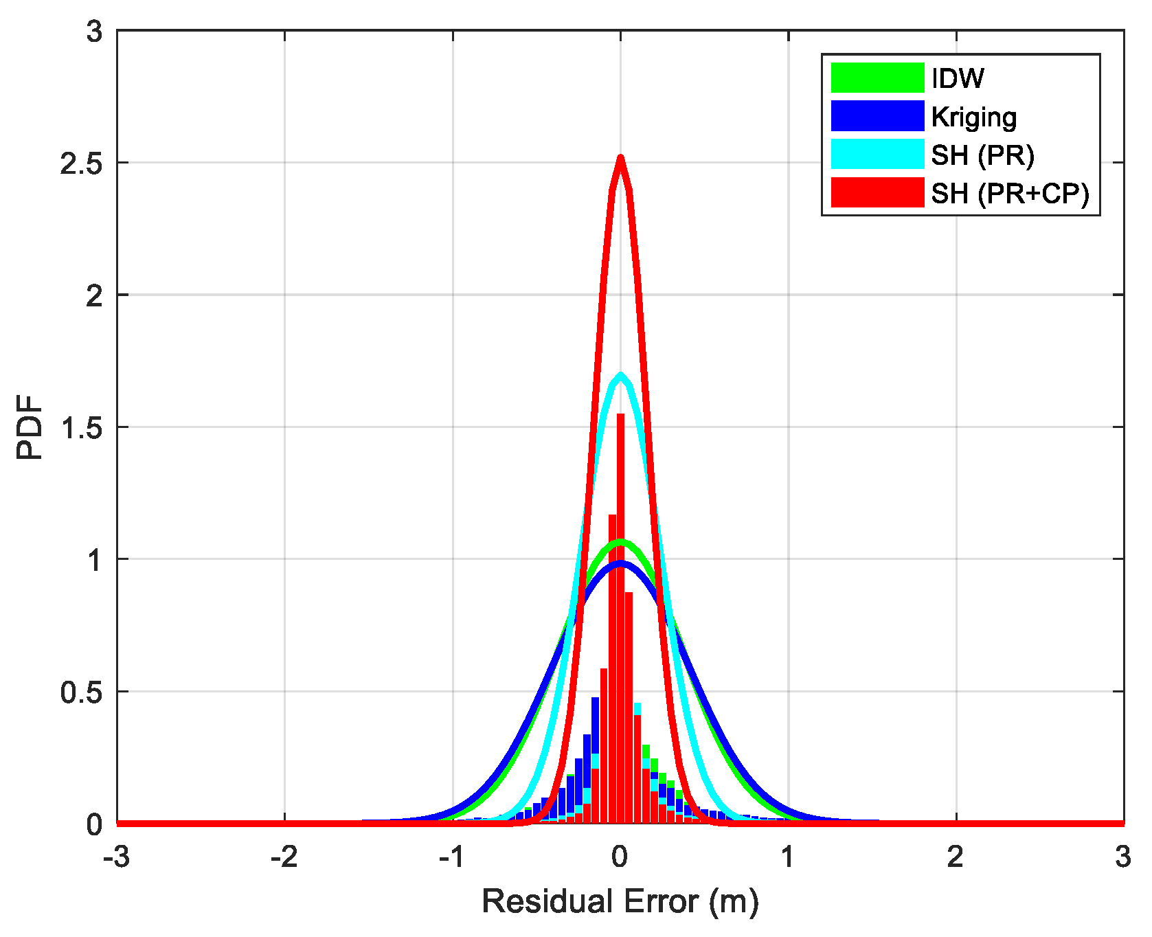
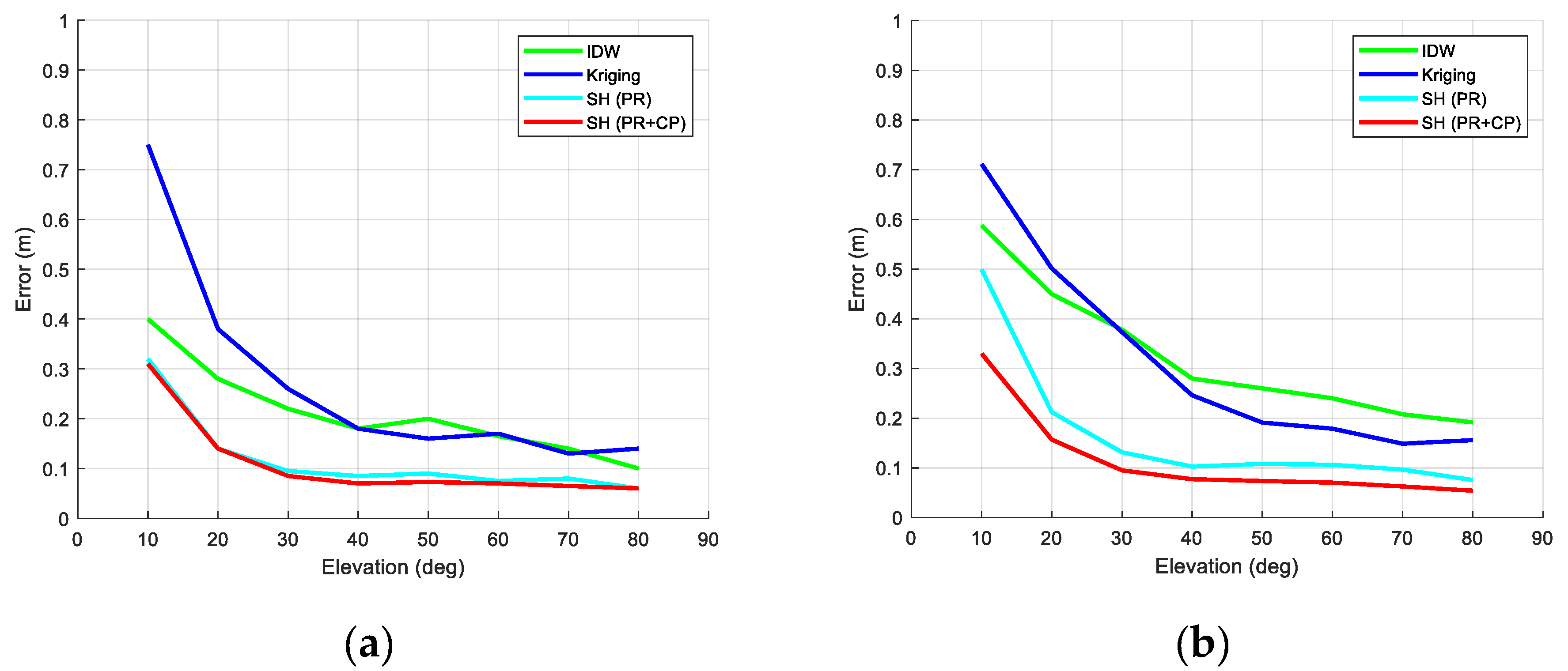
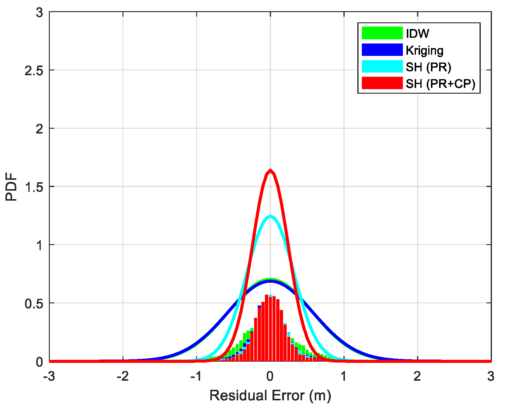
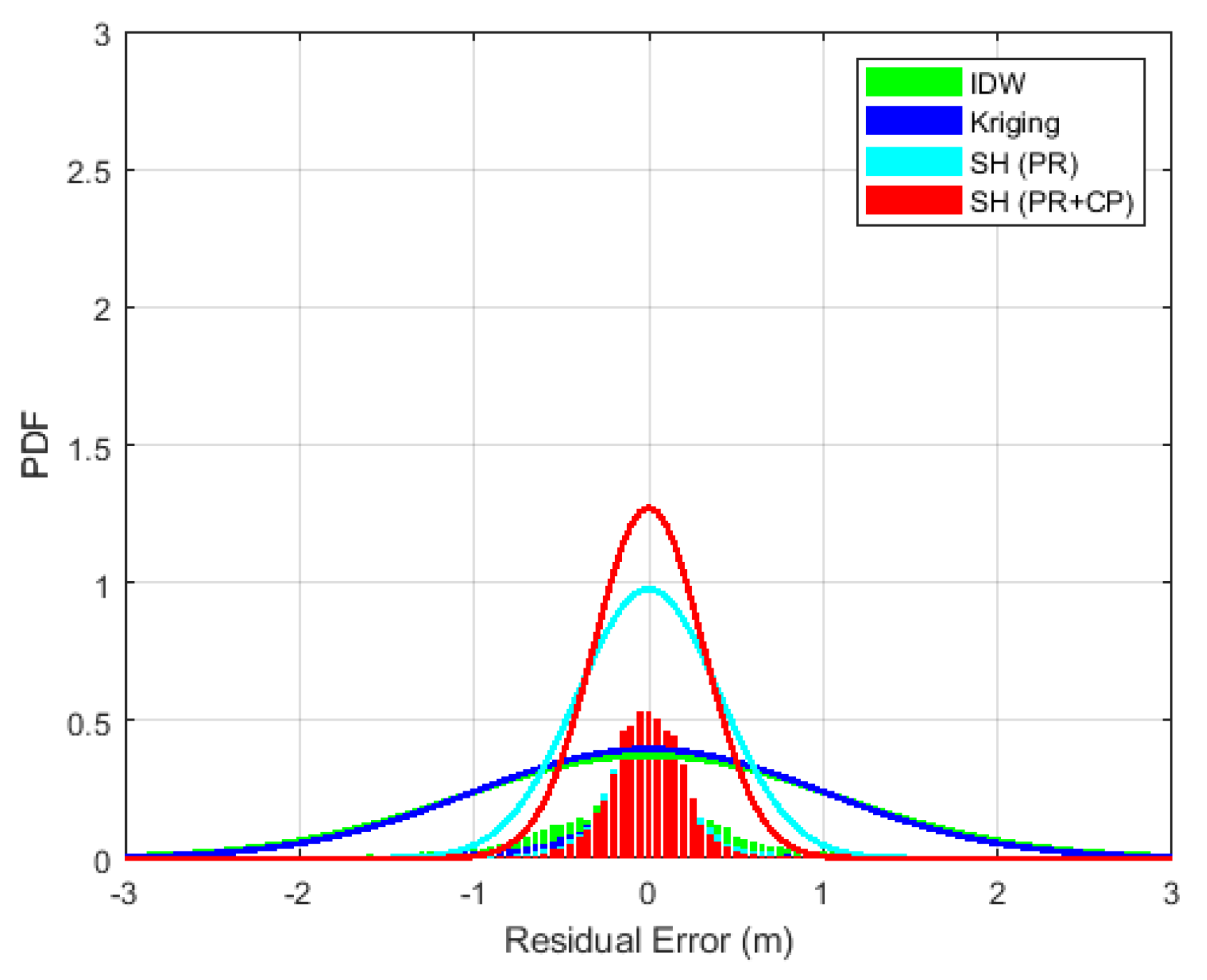
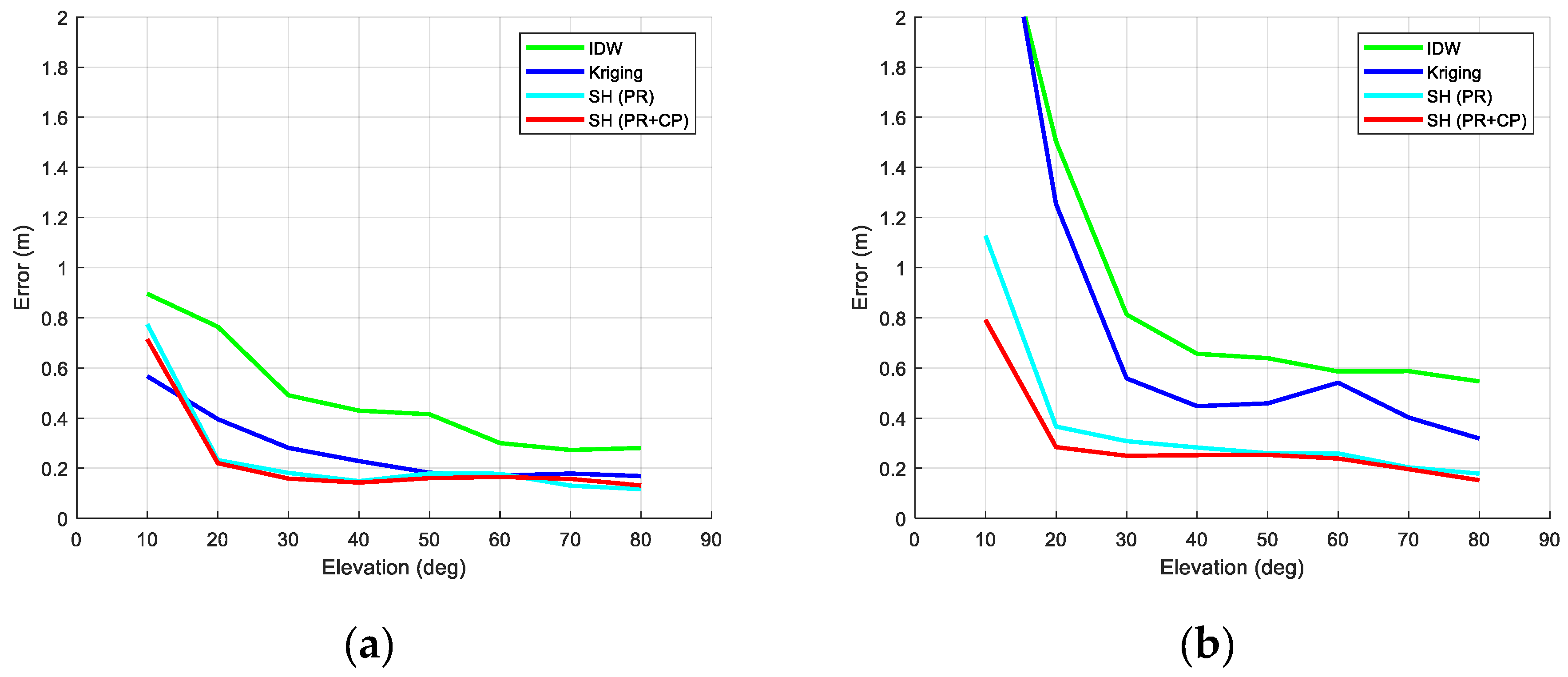
If multiple reference stations and satellites are assumed, an observation matrix can be constructed that uses all pseudorange and carrier phase measurements. Equations (14)–(16) are the measurement vectors:

$$z={\left[\begin{array}{cc}{z}_{\rho }{}^T& z_{\Delta \nabla \varphi }{}^T\end{array}\right]}^T$$

(14)

$$z_{\rho }={\left[\begin{array}{ccccc}{\left(I_{\rho }\right)}_1^1& {\left(I_{\rho }\right)}_1^2& \cdots & {\left(I_{\rho }\right)}_i^j& \cdots \end{array}\right]}^T$$

(15)

$$z_{\Delta \nabla \varphi }={\left[\begin{array}{ccccc}{}_1{}^1\Delta {\nabla }_M^r{I}_{\varphi }& {}_1{}^2\Delta {\nabla }_M^r{I}_{\varphi }& \cdots & {}_i{}^j\Delta {\nabla }_M^r{I}_{\varphi }& \cdots \end{array}\right]}^T$$

(16)

where $z$ is the measurement vector for ionospheric modeling, $z_{\rho }$ is the pseudorange-based measurement vector, and $z_{\Delta \nabla \varphi }$ is the double-difference carrier-based measurement vector. The superscript indicates the satellite, and the subscript indicates the reference station. $M$ is the master station, and $i$ is an auxiliary station. The master station is paired with each auxiliary station for the double-difference measurement; $r$ indicates the reference satellite.

Because two types of measurement with significantly different error levels are used for the estimation, it is important to construct a covariance matrix to properly weight each measurement according to the error level. The covariance matrix of the measurements is expressed as follows:

$$V=\left[\begin{array}{cc}{V}_{\rho }& O\\ O& V_{\Delta \nabla \varphi }\end{array}\right]$$

(17)

where $V$ is the covariance matrix of all measurements, $V_{\rho }$ is the covariance matrix of the pseudorange-based measurement, and $V_{\Delta \nabla \varphi }$ is the covariance matrix of the double-difference carrier phase-based measurement. If the pseudorange and carrier phase are assumed to have no correlation, the off-diagonal terms of $V$ are zeros. The detailed elements of $V_{\rho }$ are expressed below:

$$\begin{array}{ll}{\sigma }_{l,l}{}^2& ={\sigma }_{I_{\rho }}{}^2+{\left(\frac{1}{\gamma -1}\right)}^2\cdot \left({\sigma }_{{}_{b^{Tx}}}{}^2+{\sigma }_{{}_{b^{Rx}}}{}^2\right)\\ & ={\left(\frac{1}{\gamma -1}\right)}^2\cdot \left({\sigma }_{\rho 1}{}^2+{\sigma }_{\rho 2}{}^2+{\sigma }_{{}_{b^{Tx}}}{}^2+{\sigma }_{{}_{b^{Rx}}}{}^2\right)\end{array}$$

(18)

$${\sigma }_{l,k}{}^2=\{\begin{array}{cc}0& iflandksharenocommonreceiverorsatellite\\ {\sigma }_{b^{Tx}}^{}{}^2& iflandksharecommonsatellite\\ {\sigma }_{b^{Rx}}^{}{}^2& iflandksharecommonreceiver\end{array}$$

(19)

where ${\sigma }_{l,l}{}^2$ is the diagonal element of $V_{\rho }$, ${\sigma }_{l,k}{}^2$ is an off-diagonal element of $V_{\rho }$, $l$ is a row number, $k$ is a column number, ${\sigma }_{\rho 1}{}^2$ and ${\sigma }_{\rho 2}{}^2$ are the variances of the L1 and L2 pseudorange measurement errors, respectively, and ${\sigma }_{b^{Tx}}^{}{}^2$ and ${\sigma }_{b^{Rx}}^{}{}^2$ are the variances of the estimation errors for the satellite and receiver DCBs, respectively. The noise and multipath effect of the L1 and L2 frequency pseudorange are not very different, and an empirical code noise and multipath (CNMP) model has been developed that depends on the smoothing time [30,31]. With this empirical model, ${\sigma }_{l,l}{}^2$ can be expressed as follows:

$$\begin{array}{ll}{\sigma }_{l,l}{}^2& ={\sigma }_{I_{\rho }}{}^2+{\left(\frac{1}{\gamma -1}\right)}^2\cdot \left({\sigma }_{{}_{b^{Tx}}}{}^2+{\sigma }_{{}_{b^{Rx}}}{}^2\right)\\ & ={\left(\frac{1}{\gamma -1}\right)}^2\cdot \left(2{\sigma }_{CNMP}{}^2+{\sigma }_{{}_{b^{Tx}}}{}^2+{\sigma }_{{}_{b^{Rx}}}{}^2\right)\end{array}$$

(20)

where ${\sigma }_{CNMP}{}^2$ is the empirical CNMP variance. ${\sigma }_{CNMP}$ was determined so that all the empirical errors can be bounded. Figure 3 shows ${\sigma }_{CNMP}$ against the smoothing time. Initially, it was approximately 3 m, and continuously decreased. After 12,000 s, it plateaued at a value of 0.12 m.

The elements of the covariance matrix of the double-difference measurement are expressed in Equations (21)–(24). Because the double-difference measurements were made with one master station, all measurements were related with the reference satellite of the master station. In addition, there are many correlations based on the terms shared by the measurements.

$$V_{\Delta \nabla \varphi }=\left[\begin{array}{cccccc}{\sigma }_{{}_1^1\Delta {\nabla }_M^r{I}_{\varphi }}{}^2& {\sigma }_{{}_1{\Delta }_M^r{I}_{\varphi }}{}^2& \cdots & {\sigma }_{{}^1{\nabla }_M^r{I}_{\varphi }}{}^2& {\sigma }_{{\left(I_{\varphi }\right)}_M^r}{}^2& \cdots \\ {\sigma }_{{}_1{\Delta }_M^r{I}_{\varphi }}{}^2& {\sigma }_{{}_1^2\Delta {\nabla }_M^r{I}_{\varphi }}{}^2& \cdots & {\sigma }_{{\left(I_{\varphi }\right)}_M^r}{}^2& {\sigma }_{{}^2{\nabla }_M^r{I}_{\varphi }}{}^2& \cdots \\ ⋮& ⋮& \ddots & ⋮& ⋮& \cdots \\ {\sigma }_{{}^1{\nabla }_M^r{I}_{\varphi }}{}^2& {\sigma }_{{\left(I_{\varphi }\right)}_M^r}{}^2& \cdots & {\sigma }_{{}_2^1\Delta {\nabla }_M^r{I}_{\varphi }}{}^2& {\sigma }_{{}_2{\Delta }_M^r{I}_{\varphi }}{}^2& \cdots \\ {\sigma }_{{\left(I_{\varphi }\right)}_M^r}{}^2& {\sigma }_{{}^2{\nabla }_M^r{I}_{\varphi }}{}^2& \cdots & {\sigma }_{{}_2{\Delta }_M^r{I}_{\varphi }}{}^2& {\sigma }_{{}_2^2\Delta {\nabla }_M^r{I}_{\varphi }}{}^2& \cdots \\ ⋮& ⋮& ⋮& ⋮& ⋮& \ddots \end{array}\right]$$

(21)

$${\sigma }_{{}_i^j\Delta {\nabla }_M^r{I}_{\varphi }}{}^2={\sigma }_{{\left(I_{\varphi }\right)}_i^j}{}^2+{\sigma }_{{\left(I_{\varphi }\right)}_i^r}{}^2+{\sigma }_{{\left(I_{\varphi }\right)}_M^j}{}^2+{\sigma }_{{\left(I_{\varphi }\right)}_M^r}{}^2$$

(22)

$${\sigma }_{{}_i{\Delta }_M^r{I}_{\varphi }}{}^2={\sigma }_{{\left(I_{\varphi }\right)}_i^r}{}^2+{\sigma }_{{\left(I_{\varphi }\right)}_M^r}{}^2$$

(23)

$${\sigma }_{{}^j{\nabla }_M^r{I}_{\varphi }}{}^2={\sigma }_{{\left(I_{\varphi }\right)}_M^j}{}^2+{\sigma }_{{\left(I_{\varphi }\right)}_M^r}{}^2$$

(24)

where ${\sigma }_{{\left(I_{\varphi }\right)}_i^j}{}^2$ is the variance of the carrier phase-based ionospheric delay collected from the $i$-th station and $j$-th satellite, ${\sigma }_{{}_i{\Delta }_M^r{I}_{\varphi }}{}^2$ and ${\sigma }_{{}^j{\nabla }_M^r{I}_{\varphi }}{}^2$ are the variances of the single-difference measurements for the receiver and satellite, respectively, and ${\sigma }_{{}_i^j\Delta {\nabla }_M^r{I}_{\varphi }}{}^2$ is the variance of the double-difference measurement from the $i$-th auxiliary station and $j$-th satellite.

According to Equation (9), ${\sigma }_{{\left(I_{\varphi }\right)}_i^j}{}^2$ can be expressed as follows:

$${\sigma }_{{\left(I_{\varphi }\right)}_i^j}{}^2={\left(\frac{1}{\gamma -1}\right)}^2\cdot \left({\sigma }_{{\varphi }_1}^2+{\sigma }_{\varphi 2}^2\right)$$

(25)

where ${\sigma }_{{\varphi }_1}^2$ and ${\sigma }_{{\varphi }_2}^2$ are the variances of the L1 and L2 carrier phase measurements, respectively. The carrier phase had a much smaller measurement error than the pseudorange with a noise error of millimeters and multipath error of centimeters. The maximum size of the multipath error can reach a quarter of its wavelength [32]. To conservatively bound the error, the 3-sigma of the L1 and L2 carrier phase measurement errors was set to a quarter of each wavelength. That is, one sigma was set to 1.6 cm for the L1 signal and 2 cm for the L2 signal.

The collected measurements were used to estimate the spherical harmonics coefficients. Equations (26) and (27) show the coefficient vector and observation equation, respectively:

$$x={\left[\begin{array}{cccc}{C}_{00}& \cdots & C_{NN}& S_{NN}\end{array}\right]}^T$$

(26)

$$\begin{array}{l}z=Hx\\ =\left[\begin{array}{c}{H}_{\rho }\\ H_{\Delta \nabla \varphi }\end{array}\right]x\end{array}$$

(27)

where $x$ is the coefficient vector, $H$ is the full observation matrix, $H_{\rho }$ is the observation matrix for the pseudorange-based ionospheric delay measurement, and $H_{\Delta \nabla }$ is the observation matrix for the double-difference carrier phase-based ionospheric delay measurement. The detailed elements of the observation matrix for the pseudorange and double-difference carrier phase measurement are given below:

$$H_{\rho }=\left[\begin{array}{cccc}{P}_{00}(\sin {\theta }_1^1)\cdot \cos (0\cdot {\lambda }_1^1)\cdot {\mathrm{Q}}_1^1& \cdots & P_{NN}(\sin {\theta }_1^1)\cdot \cos (\mathrm{m}\cdot {\lambda }_1^1)\cdot {\mathrm{Q}}_1^1& P_{NN}(\sin {\theta }_1^1)\cdot \sin (\mathrm{m}\cdot {\lambda }_1^1)\cdot {\mathrm{Q}}_1^1\\ P_{00}(\sin {\theta }_1^2)\cdot \cos (0\cdot {\lambda }_1^2)\cdot {\mathrm{Q}}_1^2& \cdots & P_{NN}(\sin {\theta }_1^2)\cdot \cos (\mathrm{m}\cdot {\lambda }_1^2)\cdot {\mathrm{Q}}_1^2& P_{NN}(\sin {\theta }_1^2)\cdot \cos (\mathrm{m}\cdot {\lambda }_1^2)\cdot {\mathrm{Q}}_1^2\\ ⋮& ⋮& ⋮& ⋮\\ P_{00}(\sin {\theta }_i^j)\cdot \cos (0\cdot {\lambda }_i^j)\cdot {\mathrm{Q}}_i^j& \cdots & P_{NN}(\sin {\theta }_i^j)\cdot \cos (\mathrm{m}\cdot {\lambda }_i^j)\cdot {\mathrm{Q}}_i^j& P_{NN}(\sin {\theta }_i^j)\cdot \cos (\mathrm{m}\cdot {\lambda }_i^j)\cdot {\mathrm{Q}}_i^j\\ ⋮& ⋮& ⋮& ⋮\end{array}\right]$$

(28)

$$H_{\Delta \nabla \varphi }=\left[\begin{array}{cccc}{}_1^1\Delta {\nabla }_M^r\left\{P_{00}(\sin \theta )\cdot \cos (0\cdot \lambda )\cdot \mathrm{Q}\right\}& \cdots & {}_1^1\Delta {\nabla }_M^r\left\{P_{NN}(\sin \theta )\cdot \cos (\mathrm{m}\cdot \lambda )\cdot \mathrm{Q}\right\}& {}_1^1\Delta {\nabla }_M^r\left\{P_{NN}(\sin \theta )\cdot \sin (\mathrm{m}\cdot \lambda )\cdot \mathrm{Q}\right\}\\ {}_1^2\Delta {\nabla }_M^r\left\{P_{00}(\sin \theta )\cdot \cos (0\cdot \lambda )\cdot \mathrm{Q}\right\}& \cdots & {}_1^2\Delta {\nabla }_M^r\left\{P_{NN}(\sin \theta )\cdot \cos (\mathrm{m}\cdot \lambda )\cdot \mathrm{Q}\right\}& {}_1^2\Delta {\nabla }_M^r\left\{P_{NN}(\sin \theta )\cdot \cos (\mathrm{m}\cdot \lambda )\cdot \mathrm{Q}\right\}\\ ⋮& & ⋮& ⋮\\ & & & \end{array}\right]$$

(29)

With the above measurement equation and covariance matrix, the weighted least-square estimation equation is expressed as follows:

$$\widehat{x}=\left(H^T{V}^{-1}{H}^T\right)H^T{V}^{-1}z$$

(30)

where $\widehat{x}$ is the estimated coefficient vector.

If a user has coefficients, they can use them directly to reconstruct the estimated ionospheric delay map. The estimated coefficients were assumed to be delivered to the user as correction data. Then, the user can calculate the ionospheric correction by substituting the locations of IPPs into Equation (12).

4. Test Results

Tests were carried out with simulation and real data to verify the improvement with the proposed method. Reference stations and users were selected for an augmentation system in South Korea. An ionospheric correction was generated with five reference stations and the accuracy was analyzed. Only GPS satellites were used in this test. Methods using the pseudorange only were also implemented for comparison with the proposed method. The main comparison target was a spherical harmonics model that used only the pseudorange. Two grid-based algorithms were also implemented: IDW and Kriging. Under the assumption of a real-time process, correction data were estimated every epoch from measurements taken at the corresponding time.

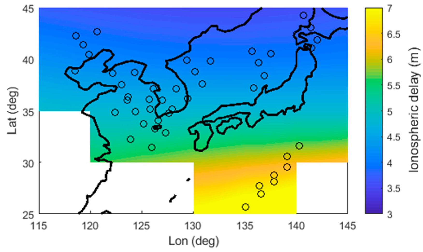
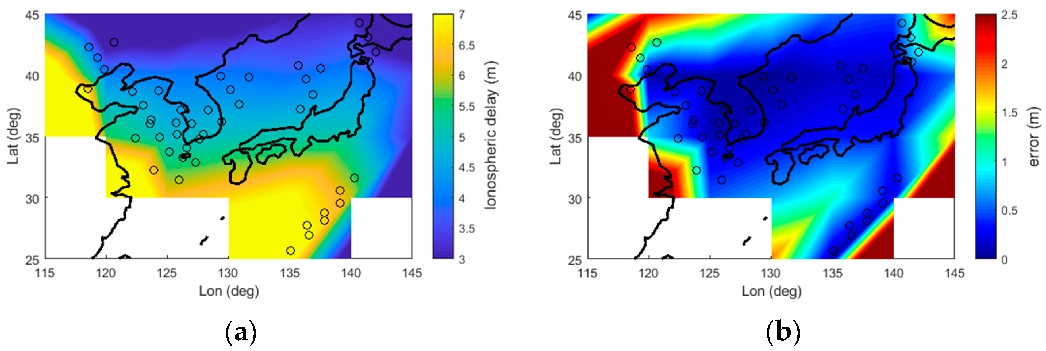
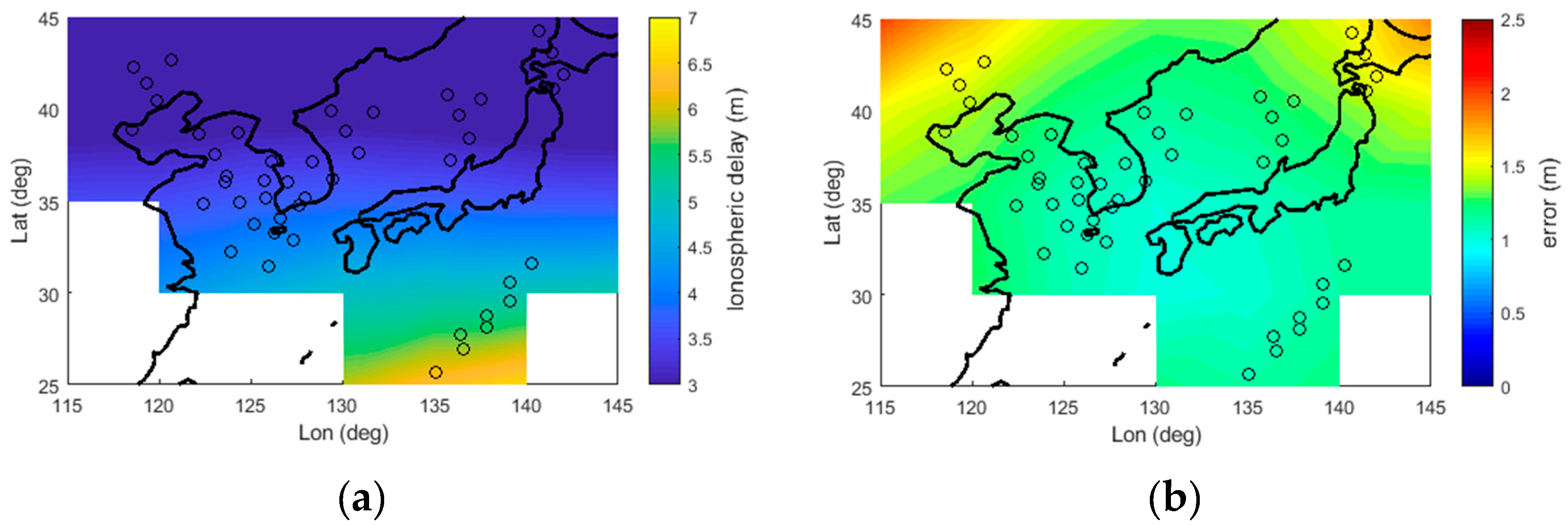
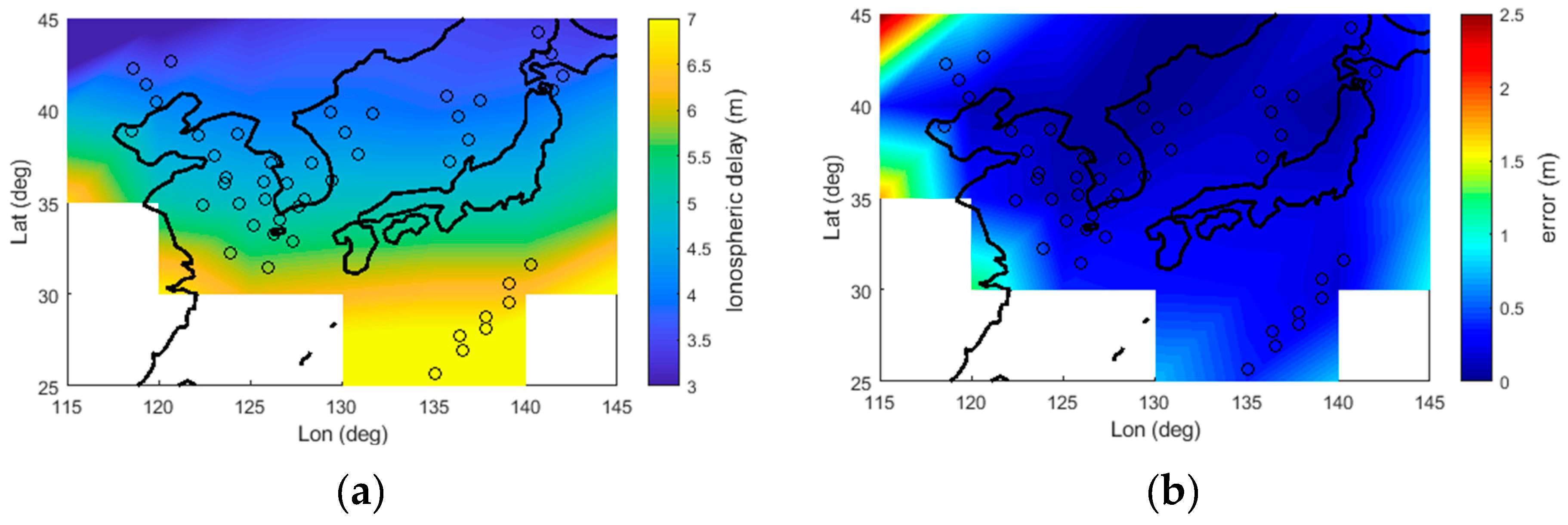
4.1. Simulation Test

Figure 4 shows the reference stations and users for the simulation test. The reference stations were set equal to those used for the test with actual data. To improve the reliability of results, multiple users across all service areas were selected. The users were uniformly distributed over the reference station network, and their numbers are shown in the figure. Simulation data were generated using IONosphere map EXchange (IONEX) format data [33]. On 1 September 2014, the simulation data were generated for 12 h in the day time (9 AM to 9 PM). The satellite positions during the test period were used to calculate the IPPs of the reference stations and users, and ionospheric delays were generated by interpolation of the IONEX data.

The vertical ionospheric map results were analyzed in order to demonstrate the effect of the double-difference measurement on the ionospheric modeling. Figure 5 shows the true ionospheric map, and Figure 6, Figure 7 and Figure 8 show the modeling results. The values are the amount of delay appearing at the L1 frequency. The IPPs of all measurement are marked with dark circles. For a given ionospheric map and measurements, spherical harmonics-based modeling was carried out with only the pseudorange, only the double-difference carrier phase, and both the pseudorange and double-difference carrier phase.

Figure 6 shows the modeling results with the pseudorange only and the error. As expected, the accuracy inside the modeling area was good, and significant degradation occurred at the edge. Figure 7 shows the modeling results with the double difference only and the error. Unlike the pseudorange-only case, the errors inside and at the edges were not significantly different. The error was smaller at the edges; however, the overall results were biased, and the error inside was greater than that of the pseudorange-only case. Because this case used only differenced data, bias could occur. Figure 8 shows the modeling results using both measurements and the error. This case showed better results for all areas compared with the previous cases. The accuracy in the center was similar to that of the pseudorange-only case, and the error at the edge areas was mitigated.

The results in the user range domain were analyzed. Four different algorithms were used in this test: (1) IDW, (2) kriging, (3) spherical harmonics with the pseudorange only, and (4) spherical harmonics with both the pseudorange and double-difference carrier. The user ionospheric correction was calculated for the modeling results of each algorithm. The residual error in the user range domain was computed by comparing the true ionospheric delay with the computed user correction. For each user, the residual errors of the four different algorithms were calculated, and their RMS values are presented in

Table 1. RMS of the residual error (simulation). User 5 was located in the center and other users were located outside the network.

User	Algorithm 1	Algorithm 2	Algorithm 3	Algorithm 4 (Proposed)
User 1	0.29 m	0.35 m	0.27 m	0.15 m
User 2	0.30 m	0.36 m	0.22 m	0.14 m
User 3	0.32 m	0.36 m	0.26 m	0.15 m
User 4	0.24 m	0.38 m	0.18 m	0.15 m
User 5	0.25 m	0.38 m	0.15 m	0.15 m
User 6	0.28 m	0.38 m	0.22 m	0.16 m
User 7	0.49 m	0.48 m	0.20 m	0.15 m
User 8	0.49 m	0.48 m	0.23 m	0.16 m
User 9	0.52 m	0.48 m	0.32 m	0.19 m
Total	0.37 m	0.41 m	0.23 m	0.16 m

. All user data were collected to calculate the overall results.

Algorithm 4 (i.e., the proposed method) showed a smaller error than the other methods for all users. The RMS error of all user data for Algorithms 1–4 were 0.37, 0.41, 0.23, and 0.16, respectively. Figure 9 shows the error distribution of each algorithm. The errors were assumed to have a Gaussian distribution; the mean and standard deviation were calculated, and the probability distribution function was plotted. The green, blue, cyan, and red colors indicate the results of Algorithms 1–4, respectively.

User 5 (at the center of the region) showed the smallest difference between Algorithms 3 and 4. Because the IPP distribution of User 5 was located inwards compared with those of the other users, the pseudorange error had a relatively small effect. To clarify where improvement occurred, users were grouped, and the residual error of each group was separated by the elevation angle. Figure 10 shows the RMS error of each elevation angle interval. Figure 10a shows the results of User 5 at the center, and Figure 10b shows the results of the other users at the edges of the service area. The errors of all algorithms tended to increase as the elevation angle decreased. For User 5, Algorithm 4 provided similar results as Algorithm 3. For Users 1–4 and 6–9, the increased error at low elevation angles was more evident for Algorithms 1–3. While the other algorithms performed worse at the edges, Algorithm 4 performed relatively consistently. These results imply that the proposed algorithm can improve the accuracy of low-elevation satellites for users at edge areas.

4.2. Real Data Test

While IONEX data is useful for checking the performance in both the vertical and slant domains, it has limitations. The resolution is not sufficient for expressing both spatial and temporal details. To show the effectiveness of the proposed method in the real world, a test was carried out with an actual dataset, with five reference stations and five users. Receiver Independent Exchange Format (RINEX) data were obtained from the archives of the National Geographic Information Institute in South Korea [34]. Figure 11 shows the reference stations and users. The users were numbered as shown in the figure. All the selected reference stations were equipped with a Trimble NETR9 receiver and geodetic antenna because the users also needed high-quality measurements for accurate analysis. The position, receiver type, and antenna type of the reference stations and users are listed in

Table 2. Reference station and user information. Baseline length is listed for auxiliary stations.

Station	Receiver	Antenna	Lat (deg)	Lon (deg)	Baseline (km)
Master	Trimble NETR9	TRM59800.00	36.52221	127.30319	-
Aux 1	Trimble NETR9	TRM59800.80	37.77092	128.86823	196.30
Aux 2	Trimble NETR9	TRM59800.80	35.17309	128.04967	164.18
Aux 3	Trimble NETR9	TRM59800.00	37.71938	126.39024	155.67
Aux 4	Trimble NETR9	TRM59800.80	33.51392	126.52982	341.08
User 1	Trimble NETR9	TRM59800.80	37.27551	127.05424	-
User 2	Trimble NETR9	TRM59800.80	35.90631	128.80197	-
User 3	Trimble NETR9	TRM59800.80	36.99197	129.41300	-
User 4	Trimble NETR9	TRM55971.00	33.46780	126.90471	-

. For auxiliary stations, the baseline length is also provided.

Considering the ionospheric activity, two days were selected. First, data were collected on 1 September 2014, under quiet conditions. Next, data were collected on 12 September 2014, under more active conditions. The daily average Kp index was 2.5 for the first data and 4 for the second data. For each day, ionospheric modeling was conducted with the measurements from the reference stations. The results were applied to the users, and the residual errors were analyzed.

This study was focused on the effect of the double-difference carrier phase on ionospheric modeling. Thus, the integer ambiguity needed to be correctly resolved. To avoid unexpected results caused by wrong integers, all integers were estimated in batches using all measurements collected throughout the test. The estimated integers were validated against the double-difference residuals. DCBs were also estimated in batches, and the errors were neglected.

Unlike the simulation, showing the error in the vertical ionospheric map for the real environment was difficult because of the challenge in making a true ionospheric map. Thus, only a range domain analysis was carried out. The precise ionospheric delay of each user was required to analyze the results in the range domain. The leveled carrier phase measurement was utilized as the ground truth data when the residual errors were calculated [35,36]. For a continuous arc with no cycle slip, the integer ambiguity is constant. In addition, the hardware biases are nearly constant over time. Therefore, there is a constant bias between the pseudorange-based measurement and carrier phase measurement, which is expressed in Equations (6) and (7). These equations can be used to compute a constant bias by averaging the difference between the two measurements. Then, the leveled carrier phase measurement can be expressed as follows:

$$\begin{array}{ll}{I}_{leveled}& =I_{\varphi }+mean\left\{I_{\rho }-I_{\varphi }\right\}\\ & =I+{\epsilon }_{leveled}\end{array}$$

(31)

where $I_{leveled}$ is the leveled carrier phase ionospheric delay measurement and ${\epsilon }_{leveled}$ is the error necessary for averaging over the entire arc and can only be calculated by a post process. Because the error is much smaller than that of the pseudorange measurement, it can be used as the ground truth.

First, the test was conducted under quiet conditions. Similar to the previous simulation results,

Table 3. RMS of the residual error (real data, 1 September 2014). Users are grouped into two groups depending on their position. Users 1 and 5 were located relatively inward, and Users 2–4 were located outward.

User	Algorithm 1	Algorithm 2	Algorithm 3	Algorithm 4 (Proposed)
User 1	0.39 m	0.29 m	0.19 m	0.17 m
User 2	0.52 m	0.56 m	0.34 m	0.28 m
User 3	0.51 m	0.40 m	0.30 m	0.22 m
User 4	0.86 m	1.00 m	0.46 m	0.30 m
User 5	0.39 m	0.23 m	0.21 m	0.21 m
Users 1 and 5	0.39 m	0.26 m	0.20 m	0.19 m
Users 2–4	0.65 m	0.70 m	0.37 m	0.27 m
Total	0.57 m	0.58 m	0.32 m	0.24 m

presents the RMS of the residual error in the range domain for the real data test. Figure 12 presents the error distribution of each algorithm.

The proposed method (i.e., Algorithm 4) showed the best results for all users. The RMS errors of all user data for Algorithms 1–4 were 0.57, 0.58, 0.32, and 0.24 m, respectively. Users 1 and 5 were located relatively inward compared with the other users. With Algorithm 3, the RMS error of Users 1 and 5 was 0.20 m. On the other hand, the errors increased for users that were located outward. The RMS error of Users 2–4 was 0.37 m. With Algorithm 4, the RMS error of Users 1 and 5 was 0.19 m, which is not significantly different from that of Algorithm 3. However, the algorithms showed differences for Users 2–4. The proposed algorithm mitigated the increased error, and the RMS error of Users 2–4 was 0.27 m.

Figure 13 shows the relation between the error and elevation angle. Similar to the simulation results, the error tended to increase as the elevation angle decreased. While Algorithms 3 and 4 had similar results for Users 1 and 5, there were clear differences for Users 2–4. Above 75°, the RMS errors were 0.19 m for Algorithm 3 and 0.15 m for Algorithm 4. Around 10°, the error of Algorithm 3 increased drastically, while the degradation was mitigated with Algorithm 4 with RMS errors of 0.79 and 0.45 m, respectively.

The second test was carried out under active conditions. The test results are represented in a manner similar to the previous results.

Table 4. RMS of the residual error (real data, 12 September 2014).

User	Algorithm 1	Algorithm 2	Algorithm 3	Algorithm 4
User 1	0.39 m	0.24 m	0.16 m	0.16 m
User 2	1.26 m	1.23 m	0.49 m	0.38 m
User 3	0.95 m	0.77 m	0.39 m	0.28 m
User 4	1.56 m	1.57 m	0.56 m	0.42 m
User 5	0.56 m	0.28 m	0.22 m	0.20 m
Users 1 and 5	0.48 m	0.26 m	0.19 m	0.18 m
Users 2–4	1.28 m	1.23 m	0.49 m	0.37 m
Total	1.07 m	1.01 m	0.41 m	0.31 m

lists the RMS of the residual error in the range domain for the real data test. Figure 14 presents the error distribution of each algorithm.

Because the ionosphere was more active, the overall error increased compared with the first test. Similar to the previous results, Algorithm 4 exhibited the best results. The RMS errors of all user data for Algorithms 1–4 were 1.07, 1.01, 0.41, and 0.31 m, respectively. For Users 1 and 5, located relatively inward, Algorithm 3 and 4 showed similar results. However, Algorithm 4 showed improved results for Users 2–4, located relatively outward. The RMS errors of Algorithm 3 and 4 were 0.49 m and 0.37 m, respectively. Figure 15 shows the relation between the error and the elevation angle. Compared with the quiet day, the error further increased as the elevation angle decreased for all algorithms. However, Algorithm 4 still showed a decrease in the error for satellites with a low elevation angle. In particular, it was more evident for Uses 2–4. Around 10°, the RMS error was 1.1 m for Algorithm 3 and 0.8 m for Algorithm 4. These results clearly indicate that the proposed algorithm improved the ionospheric correction accuracy for satellites with a low elevation angle when users were at the edges of the service area.

5. Discussion

The main area of interest of this study was the edge region of the ionospheric correction map. A relatively small number of measurements are distributed across the edge region, such that the level of performance is degraded [37,38]. The small number of measurements has two adverse effects on the estimation performance. First, it increases the effect of any measurement error. When a large number of measurements are acquired, the error can be averaged, such that the influence of any measurement error will be smaller. However, when only a small number of measurements are acquired, this averaging effect is less likely to occur, such that measurement errors may have a large effect on the estimation results. In addition, the majority of the measurements made in the edge area are obtained from low-elevation satellites, which incur a relatively large error. These large errors associated with low-elevation satellites can have a considerable impact on the estimation results under this vulnerable condition. Second, an undersampling problem occurs [25,39]. To accurately estimate the shape of the ionosphere, it is desirable that measurements be collected from various locations. Measurements collected at the edge region alone are not sufficient, in that a large degree of error may arise in the correction. This problem may be more serious in situations in which the ionosphere is highly active, such as in the event of ionospheric storms. The proposed algorithm can lessen the performance degradation that results from these measurement errors. However, the problem of undersampling cannot be alleviated with the proposed method, and additional research is needed.

There are several issues that need to be addressed to further realize this research. The first is to improve the reliability and availability of ambiguity resolution for long baselines. Because there is a considerable distance between the reference stations, the spatial decorrelation of any error affects the performance of real-time ambiguity resolution [40]. If the ambiguity is incorrectly determined, the proposed algorithm can give rise to a large estimation error because it places a considerable weighting on the double-differenced carrier phase. To focus on the effectiveness of the proposed ionospheric modeling algorithms, we used pre-estimated results with a batch process preventing any unexpected errors caused by the ambiguity being incorrect. To enable the application of the new algorithm to a real-time augmentation system, this problem must be overcome. Second, a comparison with existing algorithms considering message capacity is needed. The results presented herein were obtained by directly applying the estimated ionospheric map to the users. Depending on the application, the data rate may be limited. For example, the data rate of SBAS is only 250 bps [41]. As such, there is a need to apply a correction message according to the message standard and to analyze the result that appears when it is transmitted to the user at the actual transmission rate. Third, it is necessary to find the optimal weighting for each measurement. In this study, the variance of each measurement was assigned conservatively. It is expected that accuracy could be further improved if a measurement model that reflects the actual error level of each measurement was applied. Finally, in addition to accuracy, integrity performance is also an important factor affecting the augmentation system. The integrity problem of the algorithm should be investigated by utilizing as much long-term data as possible.

6. Conclusions

An ionospheric modeling algorithm is proposed that uses both the pseudorange and double-difference carrier phase measurement. When the ionospheric correction is generated with only the pseudorange, the performance is degraded for users at the edges of the service area, particularly for satellites with a low elevation angle. The proposed algorithm mitigated this degradation and provided relatively consistent results. The improvement was verified through tests using simulation and real data. The proposed algorithm showed the smallest error in all tests. Especially, it was more effective for satellites with a low elevation angle. In the real data test, the error decreased by about 50% for a quiet day and 30% for an active day.

While the proposed algorithm could improve the ionospheric correction accuracy, there are several issues with regard to its application in an augmentation system. The reference stations were located several hundred kilometers apart, and the wrong integer could be estimated. Because a wrong integer can generate a large error, robust real-time estimation and validation of the integer ambiguity should be implemented. Further analysis should also be carried out regarding the message bandwidth.

References

1. Klobuchar, J.A. Design and characteristics of the GPS ionospheric time delay algorithm for single frequency users. In Proceedings of the Position Location and Navigation Symposium, Las Vegas, NV, USA, 4–7 November 1986; IEEE: New York, NY, USA, 1986; pp. 280–286. [Google Scholar]
2. Kaplan, E.; Hegarty, C. Understanding GPS: Principles and Applications; Artech House: Norwood, MA, USA, 2005. [Google Scholar]
3. Kee, C.; Parkinson, B.W.; Axelrad, P. Wide area differential GPS. Navigation 1991, 38, 123–145. [Google Scholar] [CrossRef]
4. Odijk, D. Improving ambiguity resolution by applying ionosphere corrections from a permanent GPS array. Earth Planets Space 2000, 52, 675–680. [Google Scholar] [CrossRef] [Green Version]
5. Al-Shaery, A.; Lim, S.; Rizos, C. Investigation of different interpolation models used in Network-RTK for the virtual reference station technique. J. Glob. Position. Syst. 2011, 10, 136–148. [Google Scholar] [CrossRef]
6. Paziewski, J. Study on desirable ionospheric corrections accuracy for network-RTK positioning and its impact on time-to-fix and probability of successful single-epoch ambiguity resolution. Adv. Space Res. 2016, 57, 1098–1111. [Google Scholar] [CrossRef]
7. Wielgosz, P.; Krankowski, A.; Sieradzki, R.; Grejner-Brzezinska, D. Application of Predictive Regional Ionosphere Model to Medium Range RTK Positioning. Acta Geophys. 2008, 56, 1147–1161. [Google Scholar] [CrossRef]
8. Tu, R.; Zhang, Q.; Huang, G.; Zhao, H. On ionosphere-delay processing methods for single-frequency precise-point positioning. Geod. Geodyn. 2011, 2, 71–76. [Google Scholar] [Green Version]
9. Hoque, M.M.; Jakowski, N. Mitigation of ionospheric mapping function error. In Proceedings of the 26th International Technical Meeting of the Satellite Division of the Institute of Navigation, Nashville, TN, USA, 16–20 September 2013; ION: Manassas, VA, USA, 2013; pp. 1848–1855. [Google Scholar]
10. Skone, S.; Yousuf, R.; Coster, A. Performance evaluation of the wide area augmentation system for ionospheric storm events. Positioning 2004, 1, 251–258. [Google Scholar] [CrossRef]
11. Townsend, B.; Fenton, P. A practical approach to the reduction of pseudorange multipath errors in a L1 GPS receiver. In Proceedings of the 7th International Technical Meeting of the Satellite Division of the Institute of Navigation, Salt Lake City, UT, USA, 20–23 September 1994; ION: Manassas, VA, USA, 1994. [Google Scholar]
12. Simsky, A.; Sleewaegen, J.-M.; Nemry, P. Early performance results for new Galileo and GPS signals-in-space. In Proceedings of the ENC-GNSS, Manchester, UK, 7–10 May 2006; Royal Institute of Navigation: London, UK, 2006. [Google Scholar]
13. Schaer, S.; Beutler, G.; Mervart, L.; Rothacher, M.; Wild, U. Global and regional ionosphere models using the GPS double difference phase observable. Available online: https://mediatum.ub.tum.de/doc/1365730/file.pdf (accessed on 7 August 2019).
14. Han, D. A Study on Improving the Accuracy of SBAS Ionosphere Correction by Applying Double-Difference Carrier Phase Measurements. Ph.D. Thesis, Seoul National University, Seoul, Korea, 2018. [Google Scholar]
15. Hatch, R. The synergism of GPS code and carrier measurements. In Proceedings of the 3rd International Geodetic Symposium on Satellite Doppler Positioning, Las Cruces, NM, USA, 8–12 February 1982; New Mexico State University: Las Cruces, NM, USA, 1983; pp. 1213–1231. [Google Scholar]
16. Kee, C.; Walter, T.; Enge, P.; Parkinson, B. Quality control algorithms on WAAS wide-area reference stations. Navigation 1997, 44, 53–62. [Google Scholar] [CrossRef]
17. Cai, C.; Liu, Z.; Xia, P.; Dai, W. Cycle Slip Detection and Repair for Undifferenced GPS Observations under High Ionospheric Activity. GPS Solut. 2013, 17, 247–260. [Google Scholar] [CrossRef]
18. Kim, D.; Song, J.; Yu, S.; Kee, C.; Heo, M. A New Algorithm for High-Integrity Detection and Compensation of Dual-Frequency Cycle Slip under Severe Ionospheric Storm Conditions. Sensors 2018, 18, 3654. [Google Scholar] [CrossRef]
19. Park, B.; Lim, C.; Yun, Y.; Kim, E.; Kee, C. Optimal Divergence-Free Hatch Filter for GNSS Single-Frequency Measurement. Sensors 2017, 17, 448. [Google Scholar] [CrossRef] [PubMed]
20. Liu, T.; Zhang, B.; Yuan, Y.; Li, Z.; Wang, N. Multi-GNSS triple-frequency differential code bias (DCB) determination with precise point positioning (PPP). J. Geod. 2018, 93, 765–784. [Google Scholar] [CrossRef]
21. Han, D.; Kim, D.; Kee, C. Improving performance of GPS satellite DCB estimation for regional GPS networks using long-term stability. GPS Solut. 2018, 22, 13. [Google Scholar] [CrossRef]
22. Jin, R.; Jin, S.; Feng, G. M_DCB: Matlab code for estimating GNSS satellite and receiver differential code biases. GPS Solut. 2012, 16, 541–548. [Google Scholar] [CrossRef]
23. Song, J. A Study on Improving Performance of Network RTK through Tropospheric Modeling for Land Vehicle Applications. Ph.D. Thesis, Seoul National University, Seoul, Korea, 2016. [Google Scholar]
24. Gao, Y.; Petit, G.; Schaer, S. Session on Calibration and Future Receiver Developments. In Proceedings of the IGS Workshop 2008, Miami Beach, FL, USA, 2–6 June 2008. [Google Scholar]
25. Walter, T.; Hansen, A.; Blanch, J.; Enge, P.; Mannucci, T.; Pi, X.; Sparks, L.; Iijima, B.; El-Arini, B.; Lejeune, R. Robust detection of ionospheric irregularities. Navigation 2001, 48, 89–100. [Google Scholar] [CrossRef]
26. Chao, Y.-C. Real Time Implementation of the Wide Area Augmentation System for the Global Positioning System with an Emphasis on Ionospheric Modeling. Ph.D. Thesis, Stanford University, Stanford, CA, USA, 1997. [Google Scholar]
27. Sparks, L.; Blanch, J.; Pandya, N. Estimating ionospheric delay using kriging: 1. methodology. Radio Sci. 2011, 46, 1–13. [Google Scholar] [CrossRef]
28. Gao, Y.; Liu, Z.Z. Precise ionosphere modeling using regional GPS network data. J. Glob. Position. Syst. 2002, 1, 18–24. [Google Scholar] [CrossRef]
29. Moon, Y. Evaluation of 2Dimensional Ionosphere Models for National and Regional GPS Networks in Canada. Master’s Thesis, University of Calgary, Calgary, AB, Canada, 2004. [Google Scholar]
30. Shallberg, K.; Shloss, P.; Altshuler, E.; Tahmazyan, L. WAAS measurement processing, reducing the effects of multipath. In Proceedings of the 14th International Technical Meeting of the Satellite Division of the Institute of Navigation, Salt Lake City, UT, USA, 11–14 September 2001; ION: Manassas, VA, USA, 2001. [Google Scholar]
31. Shallberg, K.; Sheng, F. WAAS measurement processing; current design and potential improvements. In Proceedings of the 2008 IEEE/ION Position, Location and Navigation Symposium, Monterey, CA, USA, 5–8 May 2008; IEEE: Piscataway, NJ, USA, 2008. [Google Scholar]
32. Lau, L.; Cross, P. Development and testing of a new ray-tracing approach to GNSS carrier-phase multipath modelling. J. Geod. 2007, 81, 713–732. [Google Scholar] [CrossRef]
33. Feltens, J.; Schaer, S. IGS products for the ionosphere. In Proceedings of the 1998 IGS Analysis Center Workshop, Darmstadt, Germany, 9–11 February 1998; Available online: http://gauss.gge.unb.ca/IGS/final/ionopp98.pdf (accessed on 7 August 2019).
34. Gurtner, W.; Estey, L. RINEX: The Receiver Independent Exchange Format Version 2.11. 2012. Available online: ftp://igs.org/pub/data/format/rinex211.txt (accessed on 27 June 2019).
35. Jung, S.; Lee, J. Long-term ionospheric anomaly monitoring for ground based augmentation systems. Radio Sci. 2012, 47, 1–12. [Google Scholar] [CrossRef]
36. Nie, Z.; Zhou, P.; Liu, F.; Wang, Z.; Gao, Y. Evaluation of Orbit, Clock and Ionospheric Corrections from Five Currently Available SBAS L1 Services: Methodology and Analysis. Remote Sens. 2019, 11, 411. [Google Scholar] [CrossRef]
37. Blanch, J. Using Kriging to Bound Satellite Ranging Errors Due to the Ionosphere. Ph.D. Thesis, Stanford University, Stanford, CA, USA, 2003. [Google Scholar]
38. Sakai, T.; Kitamura, M.; Aso, T.; Hoshino, K. Avoiding Improper Modeling in SBAS Ionospheric Correction with Shrunk Observations. In Proceedings of the 2018 International Technical Meeting of the Institute of Navigation, Reston, VA, USA, 29 January–1 February 2018; ION: Manassas, VA, USA, 2018. [Google Scholar]
39. Datta-Barua, S. Ionospheric Threats to Space-Based Augmentation System Development. In Proceedings of the 17th International Technical Meeting of the Satellite Division of the Institute of Navigation (ION GNSS 2004), Long beach, CA, USA, 21–24 September 2004; ION: Manassas, VA, USA, 2004. [Google Scholar]
40. Feng, Y.; Wang, J. GPS RTK Performance Characteristics and Analysis. J. Glob. Position. Syst. 2010, 7, 1–8. [Google Scholar] [CrossRef]
41. DO-229D. WAAS MOPS (Minimum Operational Performance Standards for Global Positioning System/Wide Area Augmentation System Airborne Equipment); RTCA, Inc.: Washington, DC, USA, 2006. [Google Scholar]
Figure 1. Ionospheric modeling example using (a) pseudorange only and (b) pseudorange and double-difference carrier phase.
Remotesensing 11 01849 g001
Figure 2. Ionospheric modeling procedure. DCB: differential code bias.
Remotesensing 11 01849 g002
Figure 3. One sigma of code noise and multipath (CNMP) against the smoothing time.
Remotesensing 11 01849 g003
Figure 4. Reference station and user (simulation).
Remotesensing 11 01849 g004
Figure 5. True ionospheric map.
Remotesensing 11 01849 g005
Figure 6. (a) Estimated ionospheric map and (b) its error in the case using only the pseudorange.
Remotesensing 11 01849 g006
Figure 7. (a) Estimated ionospheric map and (b) its error in the case using only the double-difference carrier phase.
Remotesensing 11 01849 g007
Figure 8. (a) Estimated ionospheric map and (b) its error in the case using both the pseudorange and double-difference carrier phase.
Remotesensing 11 01849 g008
Figure 9. Probability distribution function for the residual error of each algorithm (simulation). IDW: inverse distance weight, SH (PR): spherical harmonics using only the pseudorange, SH (PR+CP): spherical harmonics using both the pseudorange and double difference carrier phase.
Remotesensing 11 01849 g009
Figure 10. Residual error according to the elevation angle (simulation): (a) User 5; (b) Users 1–4 and 6–9.
Remotesensing 11 01849 g010
Figure 11. Reference station and user (real data).
Remotesensing 11 01849 g011
Figure 12. Probability distribution function (PDF) for the residual error of each algorithm (real data, 1 September 2014).
Remotesensing 11 01849 g012
Figure 13. Residual error according to the elevation angle (real data, 1 September 2014): (a) Users 1 and 5; (b) Users 2–4.
Remotesensing 11 01849 g013
Figure 14. Probability distribution function for the residual error of each algorithm (real data, 1 September 2014).
Remotesensing 11 01849 g014
Figure 15. Residual error according to the elevation angle (real data, 12 September 2014): (a) Users 1 and 5; (b) Users 2–4.
Remotesensing 11 01849 g015