Article

Diagnosis of Xinmo (China) Landslide Based on Interferometric Synthetic Aperture Radar Observation and Modeling

1
School of Geology Engineering and Geomatics, Chang’an University, Xi’an 710054, China
2
Roy M. Huffington Department of Earth Sciences, Southern Methodist University, Dallas, TX 75275, USA
*
Author to whom correspondence should be addressed.
Remote Sens. 2019, 11(16), 1846; https://doi.org/10.3390/rs11161846
Submission received: 12 July 2019 / Revised: 4 August 2019 / Accepted: 6 August 2019 / Published: 8 August 2019
(This article belongs to the Special Issue Remote Sensing of Landslides II)

Abstract

:
The Xinmo landslide occurred on 24 June 2017 and caused huge casualties and property losses. As characteristics of spatiotemporal pre-collapse deformation are a prerequisite for further understanding the collapse mechanism, in this study we applied the interferometric synthetic aperture radar (InSAR) technique to recover the pre-collapse deformation, which was further modeled to reveal the mechanism of the Xinmo landslide. Archived SAR data, including 44 Sentinel-1 A/B data and 20 Envisat/ASAR data, were used to acquire the pre-collapse deformation of the Xinmo landslide. Our results indicated that the deformation of the source area occurred as early as 10 years before the landslide collapsed. The deformation rate of source area accelerated about a month before the collapse, and the deformation rate in the week before the collapse reached 40 times the average before the acceleration. Furthermore, the pre-collapse deformation was modeled with a distributed set of rectangular dislocation sources. The characteristics of the pre-collapse movement of the slip surface were acquired, which further confirmed that a locked section formed at the bottom of the slope. In addition, the spatial-temporal characteristics of the deformation was found to have changed significantly with the development of the landslide. We suggested that this phenomenon indicated the expansion of the slip surface and cracks of the landslide. Due to the expansion of the slip surface, the locked section became a key area that held the stability of the slope. The locked section sheared at the last stage of the development, which triggered the final run-out. Our study has provided new insights into the mechanism of the Xinmo landslide.

Graphical Abstract

1. Introduction

On June 24 2017, a devastating landslide occurred in Xinmo Village, Diexi Town, Mao County, Sichuan Province, China (32°04′47″N, 103°39′46″E). The landslide runout buried 64 households, killed 10 people and 73 people were determined missing [1]. The height relief of the sliding mass was about 1000 m (from the source area to the deposition area, as shown in Figure 1), and the horizontal length of the debris flow was 2270 m [2]. The deposition area of the Xinmo landslide formed a narrow horizontal fan shape, and the buried Xinmo Village was built on the deposits of a historical old landslide (as shown in Figure 1). The elevation of the source area located on the ridge of the mountainside of the Fugui Mountain is about 3281 m above sea level (a.s.l.). The stratum at the location of the Xinmo landslide is composed of metasandstone intercalated with slate layers. The rock mass was creeping along an existing sliding plane before collapsing [1]. The area’s deep mountain-canyon landform provides conditions for the formation of long-distance debris flow. This landslide is located at the junction of the Qinghai–Tibet Plateau and the Longmenshan Alpine region with active tectonic activities; three major earthquakes have occurred during the past one hundred years [1,2,3,4]. These earthquakes have caused the creation of internal joints and cracks in the rock, which allowed for the development and shearing of the landslide [1,2,5]. Rain water and the long-term gravity effect caused the propagation of these cracks [1]. The integrity of the slope was continually damaged and a potential slip surface formed before the collapse [5].
As a technology that can accurately acquire ground deformation, interferometric synthetic aperture radar (InSAR) has been widely used to identify and monitor landslides [6,7,8,9,10]. In addition, InSAR can be used in landslide modeling based on the elastic dislocation models [11,12]. Some InSAR-based studies have been done for this Xinmo landslide. Dong et al. [13] acquired the pre-collapse deformation through Sentinel-1 and ALOS-2 InSAR. Based on Sentinel-1 data, Intrieri et al. [14] recovered the pre-collapse time-series deformation of the Xinmo landslide. Dai et al. [15] evaluated the disaster after the collapse based on Sentinel-1 SAR intensity data and estimated the terrain changes of the landslide source area. However, there are still some questions that have not been answered. First, did any deformation of the landslide occur before the monitoring period of Sentinel-1 data? In addition to this, did characteristics of the pre-collapse deformation change during the development of the landslide? Second, was this landslide triggered directly by precipitation? Third, can this landslide be modeled based on elastic dislocation models [16], and can the movement of the slip surface be estimated based on pre-collapse deformation? In order to answer these questions, we utilized InSAR analysis and the modeling of the deformation based on an elastic dislocation model.

2. Data and Method

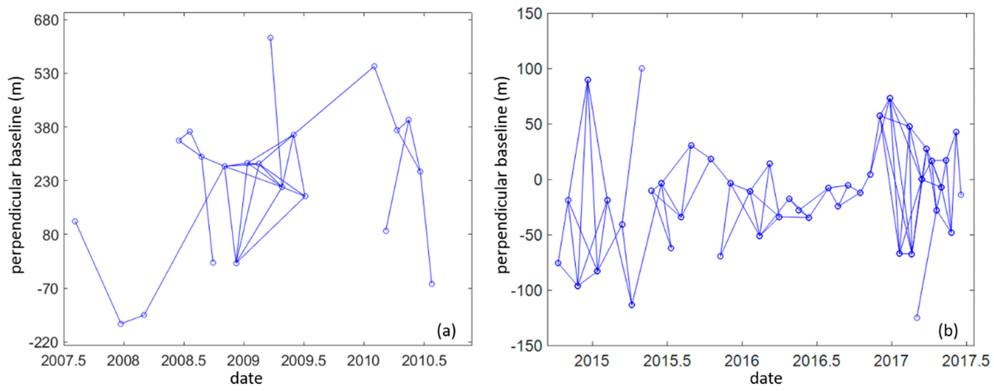
Forty-four Sentinel-1A/B and twenty-one Envisat datasets with descending orbits were used to retrieve the historical deformation of the landslide. The slope aspect of the source area was about 190 degrees from the north. Therefore, due to a larger local incidence angle, the descending data generally had higher coherence than the ascending data over the landslide [17,18]. The time span was from 6 August 2007 to 26 July 2010 for the Envisat data, and from 9 October 2014 to 19 June 2017 for the Sentinel data. By setting the spatial and temporal baseline thresholds, the interferograms configurations of these two data sets were obtained separately. Following this, after registration, filtering and unwrapping, the unwrapped interferograms could be obtained. The multi look ratios of Sentinel and Envisat data were 4:1 and 1:5 respectively, and the DEM adopted for the differential and analysis was the 30-m shuttle radar topography mission (SRTM) data. The interferograms with high coherence and no unwrapping errors in the source region were selected for further processing. The configurations of the selected interferograms are shown in Figure 2. A linear model for the elevation dependent phase components was used to remove the stratified atmospheric delay in every interferogram. Then, the phase ramps were removed by a quadratic polynomial model. Based on the selected interferograms, the average velocity and the time series deformation were obtained by stacking and SBAS InSAR, respectively [10,19].
The atmospheric delay and stochastic noise can be reduced by the stacking InSAR method effectively [10]. The average phase rate P was calculated by an average in the time domain as follows,
P = φ / t
where φ is the unwrapped phase of the selected interferogram, t is the time interval of the interferogram. The time series deformation can be estimated as follows [19],
B k = φ
where B is the design matrix, k is the deformation phase between time adjacent SAR data. An inverse method (such as singular value decomposition) had to be applied to estimate the deformation phase k . Subsequently, the cumulative deformation was obtained by a trivial integration.
Landslides exhibit elasticity under small or instantaneous deformation [20,21]. In addition, the slip surface of a landslide has many similar features to faulting [22,23], and some studies have used elastic models [16] to study landslides [11,12,21]. Thus, the elastic dislocation model was applied to model the Xinmo landslide in this study. A set of distributed rectangular dislocation sources within a homogenous elastic halfspace was used to simulate InSAR deformation, and the root mean square (RMS) misfit of the residuals (observed data minus model) were used to define the best fitting parameters [24,25,26].

3. Result

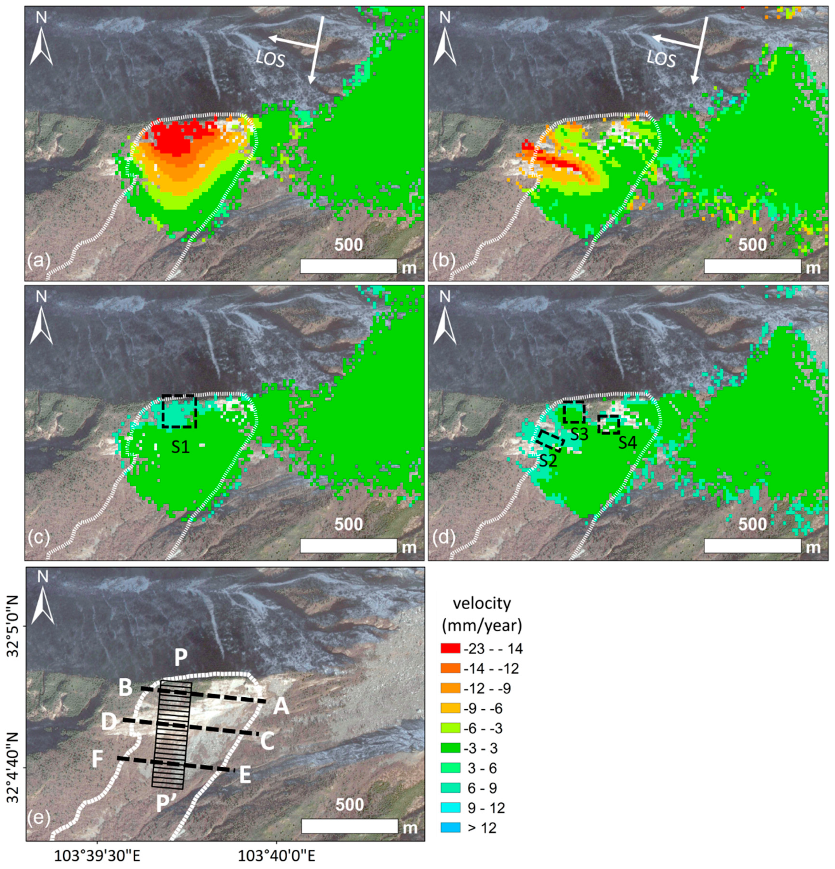
Based on the pre-collapse deformation from Sentinel-1 and Envisat data, the landslide experienced a long-term creep before the collapse. As early as June 2008, approximately 10 years before the failure, obvious deformation appeared on the upper part of the source area, in which the maximum deformation reached 1.8 cm/year in the line of sight (LOS) direction (Figure 3b).
For the Sentinel data, both the maximum slip rate and standard deviation are presented in Figure 3. The standard deviation can be an indicator of the noise and the nonlinear deformation. However, with the consideration of the short baseline and good quality of the selected Sentinel interferograms, we suggested that the large standard deviation at the top of the source area (S1 region in Figure 3c) was mainly caused by the strong nonlinear deformation. This phenomenon can indicate this region was the most unstable during October 2014 to June 2017.
The average slope aspect was about 190 degrees, which was almost parallel to the two satellite tracks; both Envisat and Sentinel-1 data are insensitive to a landslide’s down-slope movement. Therefore, most of the deformation acquired by these two satellites are from the vertical deformation of the source area. By considering that the slope of this area was nearly 40 degrees, it will produced obvious vertical deformation with the sliding of the source area. Compared with the Sentinel-1 data, Envisat data should be more sensitive to the vertical deformation, because the incidence angle of the Envisat data is smaller. However, we found that the spatial characteristics of deformation from these two data sets were quite different, and some active regions before failure did not show significant deformation during the monitoring period of the Envisat data. For the results from the Envisat data, the maximum deformation occurred in the middle of the source area. However, the maximum deformation of the Sentinel data occurred at the top of the slope, and the deformation decreased from the top to the feet of the source area gradually.
To further understand the characteristics of landslide deformation, we projected the average deformation rates to the down slope direction and extracted the deformation rates from the two data sets along three cross-sections of the landslide (as shown in Figure 3 and Figure 4). We found the results from the Sentinel data always presented a similar funnel-shaped deformation pattern. However, the Envisat data showed distinct deformation characteristics along the cross-sections. Based on the deformation in the upper and middle parts of the slope (profile AB and CD) from the Envisat data, the deformation on the west side was larger than that of the east side. Additionally, there was no obvious deformation in the west side at the foot of the source area (profile EF).

4. Discussion

4.1. Pre-Collapse Time-Series Deformation

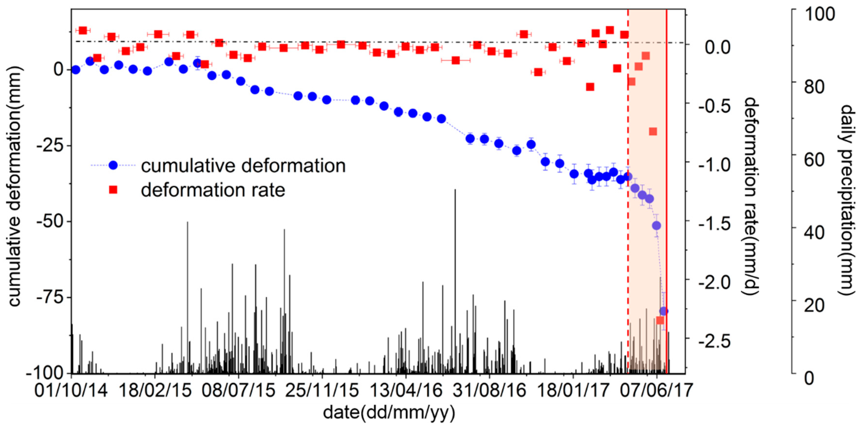
In many cases, the increase in pore water pressure caused by precipitation can reduce the landslide shear strength, which is an important external influencing factor for many landslides [27]. It has been found that there is a high correlation between the slip acceleration and the regional precipitation in many cases [7,9,27]. However, there is a time lag between the precipitation and the maximum deformation rate [6,7,28]. In order to explore the relationship between the pre-collapse deformation and precipitation, we collected historical precipitation data and analyzed it with the time–series deformation from Sentinel-1 data. The precipitation data were derived from the Global Precipitation Measurement (GPM) with a 0.1-degree spatial resolution and one-day temporal resolution. The GPM mission was initiated by the National Aeronautics and Space Administration (NASA) and the Japan Aerospace Exploration Agency (JAXA) to provide global precipitation data based on a network of satellites. The landslide was observed as having maintained a stable linear deformation before May 2017. It should be noted that the precipitation data used in this study represented an average daily rainfall with a spatial resolution of about 11 km. Therefore, this precipitation data could not reflect the actual rainfall at this particular landslide precisely. However the seasonal rainfall events in the study area could be found mainly to have occurred from May to September. However, there was no obvious acceleration in the source area during this period of 2015–2016, and there were no significant rainfall events before the acceleration. A strong correlation could not be found between the deformation rate and the rainfall events (Figure 5).
It has been shown that determining the starting point of acceleration is very important for landslide early warning studies. For example, Carlà et al. [29] used the inverse velocity method to forecast landslide collapse based on time–series monitoring data. Intrieri et al. [14] also used the same method to study the collapse time of the Xinmo landslide. As shown in Figure 5, after May 20, 2017 (the red dash line in Figure 5), the landslide deformation accelerated abruptly. It could also be found that the deformation rate of the S1 region one week before the collapse reached 2.3 mm/d, which was about 40 times higher than that during the period of non-acceleration.

4.2. Landslide Modelling

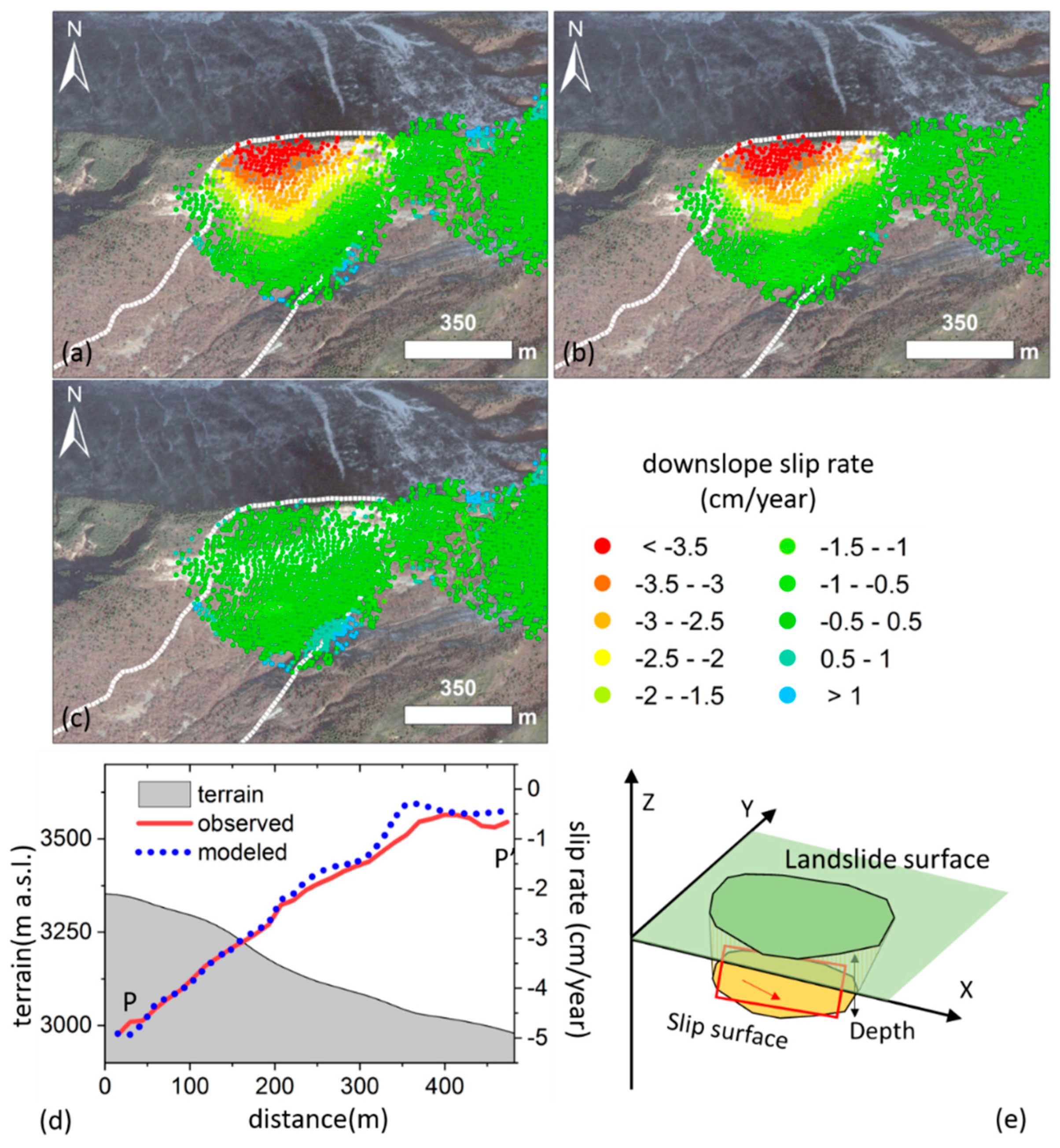
In order to further study the landslide mechanism, the elastic dislocation model [16] was applied to this landslide. Elastic dislocation models are commonly used to model static elastic deformation due to any type of slip or tensile dislocation. The Okada model in which the dislocation plane is set as a rectangle is an example of an elastic dislocation model. Since the Okada model establishes the relationship between the dislocation of the rectangular planar source below the surface and the ground displacement on the surface, this model is usually used to estimate the source parameters of some geophysical processes (e.g., earthquake, volcano and landslide). Referring to Aryal et al. [21] and Nikolaeva et al. [11], we established a simplified model, which regarded the slip surface as the Okada rectangular dislocation source. Because this landslide was classified as a bedding type and the dip angle of the bedding plane was similar to the slope of the source area [1], we set the sliding surface parallel to the average surface of the source area, as shown in Figure 6e. Then, the position and size (length: 420 m; width: 330 m; strike: 86° clockwise from the North) of an Okada rectangle was given based on the failure boundary and the deformation region. The difference in the landslide topography before and after the collapse mostly ranged between 40 and 80 m [15,31]. Therefore, we set 60 m for the depth of the slip surface, which could be regarded as the average depth of the slip surface. Finally, a set of rectangular dislocation sources were used to model the pre-collapse deformation from the Sentinel-1 data. The slip of each patch was estimated by constrained linear least-squares, and Laplacian smoothing was applied to prevent the unrealistic oscillatory slip. As shown in Figure 6, the simulated downslope deformation corresponded well with the actual observations, which further illustrated the rationality of our model.
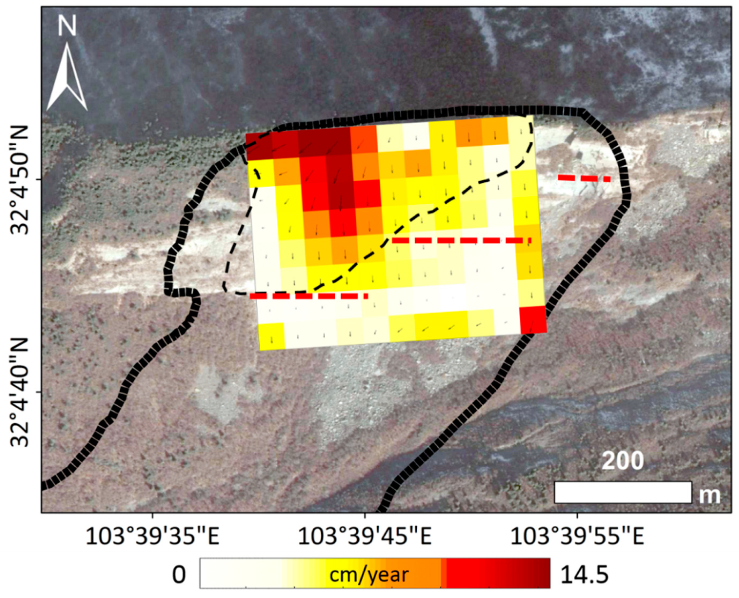
As shown in Figure 6, the slip distribution of the sliding surface can be acquired. Therefore, the ‘slip’ here represented the shear movement of each dislocation source. It can be seen that the slip distribution also showed a characteristic gradual decrease from the top to the foot of the source area. As shown in the black dashed line in Figure 7, we roughly plotted the area with elevation changes larger than 40 m before and after collapse in the landslide based on previous research [31]. The regions of the slip surface with obvious slip had a certain correlation with the main collapsed area (black dashed line in Figure 7). The maximum slip of the basal plane reached 14.5 cm/year, which was larger than that of the surface of the slope. Based on previous research, the landslide formed a locked section at the foot of the source [5]. The locked section is an intact portion of the rock mass where the sliding surface is not completely formed or is completely absent [32]. Commonly found in rocky landslides of the Southwestern mountainous area of China, one or more locked sections control the stability of the landslide. A failure of a locked section usually leads to a violent landslide with a long-distance runout [10,32,33]. The locked section of this landslide was roughly plotted. As shown in Figure 7, the movement of the slip surface below the locked section was small. We suggested that this was because the locked section was an unconnected area, in which the slip surface had not completely formed. The locked section prevented the shear movement on the basal plane. This phenomenon confirmed the rationality of the inversion results and could further indicate that the landslide formed a locked section at the foot of the slope before the collapse. However, it should be noted that the slip distribution represents a rough result, because only a one-dimensional slope deformation was acquired in this study. In addition, we assumed that the slip surface was a plane with uniform depth.

4.3. Landslide Development Analysis

Different characteristics of deformation often correspond to different mechanisms of landslides [32,33,34]. Therefore, the change in the characteristics of deformation and strain can reflect the changes of some physical properties of the landslide during its development. Hence, we wanted to know how the deformation and strain of landslides changed during the development of the landslide. Multi-dimensional deformations can be used to calculate the strain (and strain rate) of the landslide, which can indicate the landslide body’s regions of extension and compression [35,36]. However, only one-dimensional deformation of the landslide was obtained during the monitoring period. Thus, we assumed that the sliding of the landslide mainly occurred in the downslope direction and that there was little strain perpendicular to the landslide surface. Therefore, the deformation gradient along the downslope direction was used to represent the strain of the surface of the landslide. Because the deformation gradient is very sensitive to noise [35], we extracted the slope deformation rate in the rectangular polygon along the average downslope direction PP’ (Figure 3e). This rectangular polygon was then divided into 22 small rectangles (Figure 3e), and the average of the downslope deformations within each of the smaller rectangles were calculated as the representative deformation of each block. Finally, the deformation gradients along the slope direction were calculated based on the downslope deformation rate of each small rectangle:
S = v / l
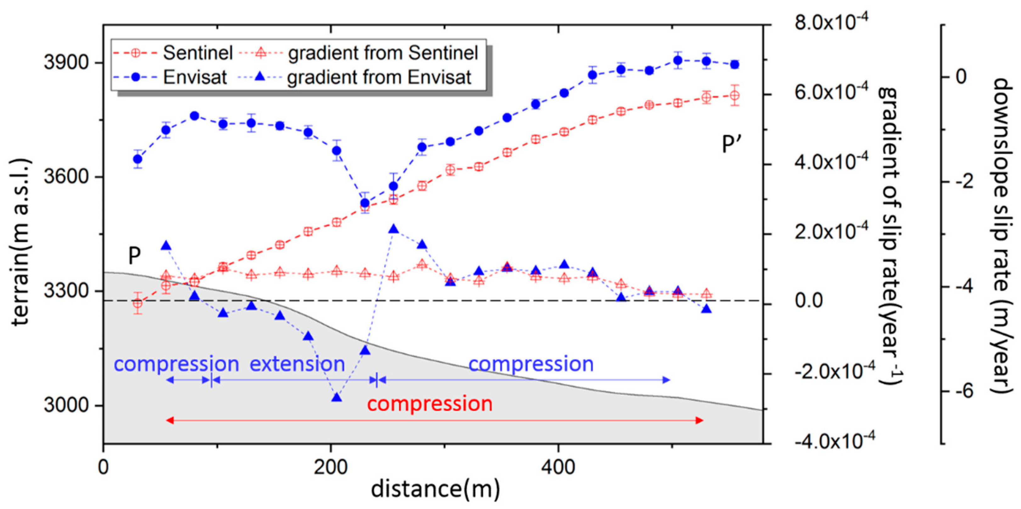
where S is the strain rate at the surface of the landslide, v is the average downslope deformation rate of each small rectangle, and l is the downslope distance. It should be noted that only a one-dimensional deformation was considered in the estimation of the gradient. Because the direction of the landslide might not be simply a downslope, we could not obtain the accurate strain rate of the source area. Therefore, only qualitative analysis was conducted based on the strain rate. As shown in Figure 8, along the slope direction, the maximum deformation from the Sentinel-1 data was located at the top of the slope, while the deformation center of the Envisat was located in the middle of the source area. As we defined the downslope deformation as negative, the positive gradient represented a characteristic of compaction in the downslope direction. We found that the entire source area surface exhibited compression during the monitoring period of the Sentinel data. While during the Envisat monitoring period, the surface of the source area exhibited compression at the top and at the feet of the slope surface, but extension was found in the middle area.
In order to further understand the changes in the deformation characteristics of this landslide, the time–series deformation of the landslide was analyzed. We found that deformation characteristics of the landslide changed significantly in the second half of 2015. Until July 12, 2015, the middle of the source still had a relatively larger deformation (as shown in Figure 9 and Figure S1). This deformation characteristic was very similar to that during the monitoring period of the Envisat data. However, this characteristic of the deformation changed gradually from July to November 2015, suggesting that the deformation decreased from the top to the foot of the source.
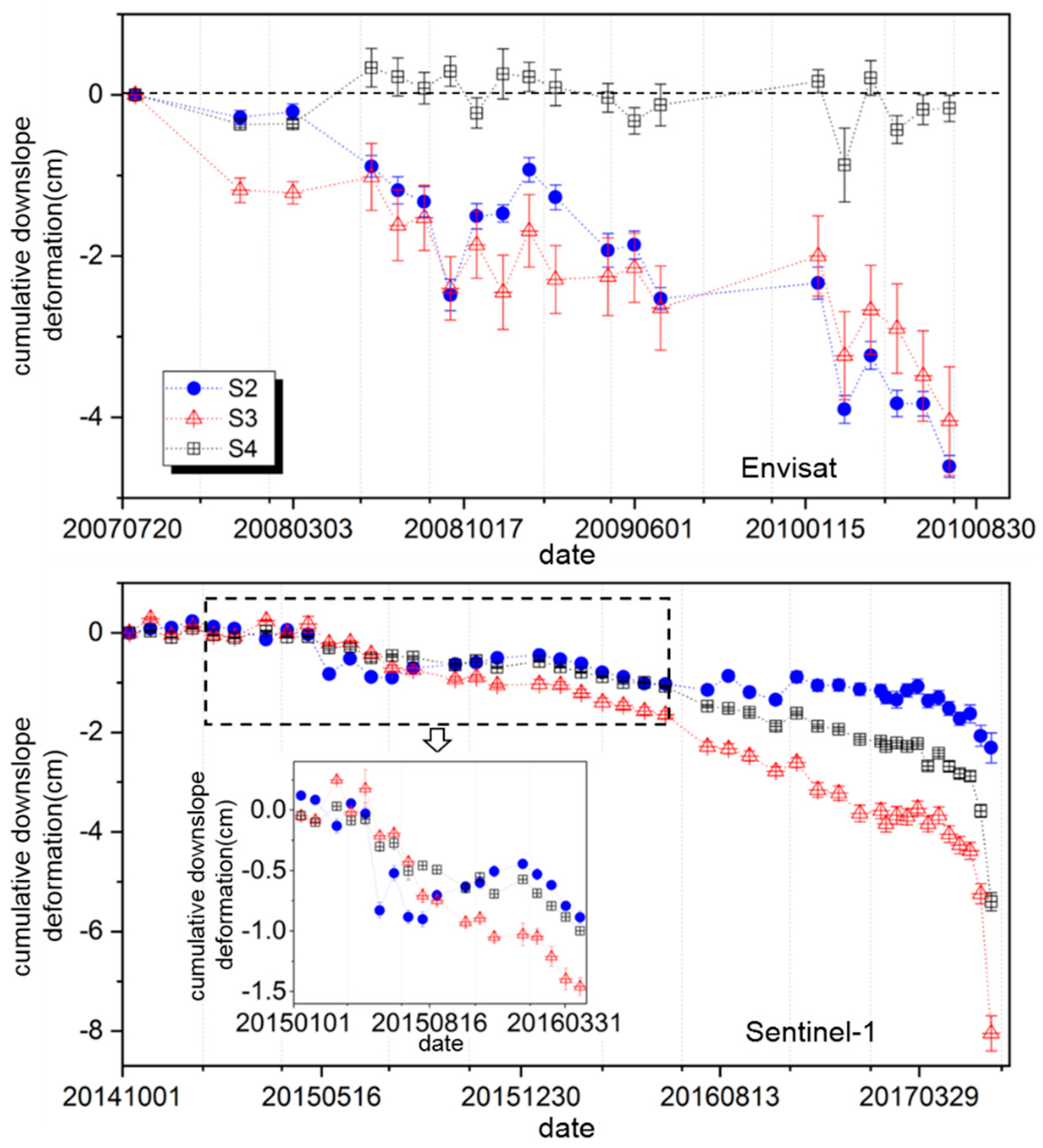
We extracted the median value of each cumulative deformation from the Envisat and Sentinel-1 data in the regions S2, S3 and S4 for analysis (the locations of these regions are as shown in Figure 3d), and used the root mean square error of the deformation in these regions as an indicator of motion heterogeneity. As shown in Figure 10 and Figure S2, there was no obvious time–series deformation in the S2 region, but the S3 and S4 regions exhibited persistent deformation during the monitoring period of the Envisat data (the locations and extents of these regions are shown in Figure 3d). However, the S2 region became an active area during the monitoring period of the Sentinel-1 data. In addition, we found that the S2 area showed a deformation characteristic of gradual uplift, while the S3 and S4 areas still showed a downward deformation during the second half of 2015 (Figure 10 (lower)).
It was found that the characteristics of deformation and strain rate changed with the development of the landslide. By considering the continuous expansion of the potential slip surface and the propagation of cracks with the development of this landslide [1,5], we suggested that these deformation characteristics and changes in strain rate corresponded to the propagation and interconnection of the cracks and the potential slip surface of this landslide. The expansion of the potential slip surface will lead to a change in the stress distribution, which, in turn, will lead to a change in the deformation characteristics ultimately. For example, during the second half of 2015, the S2 region was subject to an increased pressure from the top region of the slope (such as S3 and S4 regions) due to the propagation of the slip surface or cracks at the upper portion of the landslide. This might have caused an upward deformation of bending in the S2 region (as shown in the Figure 10 (lower panel)). Since the deformation characteristics of the landslide changed obviously in the second half of 2015, the range and connectivity of the potential slip surface and the cracks of the landslide may have changed significantly during this period.
Based on the analysis above, we constructed a simple schematic of the development of the landslide (shown in the Figure 11). Due to the history of earthquakes, the slope formed many fractures and cracks [1]. This potential slip surface gradually became interconnected with the development of the landslide. An unconnected area at the bottom of the source area formed the locked section [5]. The shear strength of the landslide could decrease significantly with the expansion of the slip surface [36]. In addition, the long-term gravitational effect and external factors such as precipitation resulted in the failure of the locked section. Then, the potential energy of the source area was released instantaneously, which caused the landslide run out.

5. Conclusions

Using Sentinel-1A/B and Envisat data, the deformation preceding the 2017 Xinmo landslide was recovered. We found that the landslide was creeping approximately 10 years before the failure. For the results from the Sentinel-1 data (9 October 2014–19 June 2017), the deformation decreased from the top to the foot of the source area gradually. However, the maximum deformation occurred in the middle of the source area from the Envisat results (16 June 2008–26 July 2010). The deformation characteristics and the strain rate of the source area changed during this past decade, particularly in mid-2015. Based on the time series deformation and precipitation data, it could be found that there was no strong correlation between the pre-collapse time series deformation and the rainfall events, and the initial acceleration date of the landslide occurred around 20 May 2017. The elastic dislocation model was used in the landslide modeling and analysis. Through a set of distributed Okada sources, the pre-collapse deformation of the landslide was modeled, and the slip distribution of the sliding surface was estimated. The inverted slip distribution had good correspondence with the main collapse zone and the locked section. It indicated that the results of modeling and the geological exploration could be mutually confirmed.
We suggested that the changes in the deformation area revealed the development of the slip surface and inter-connected cracks. The stability of the landslide decreased continuously with the expansion of the slip surface. In the last stage, the locked section at the foot of the source area sheared, which caused the tragic disaster in 2017.
The study of landslides based on a radar remote sensing technique is limited by the temporal resolution of remote sensing images. However, all-weather radar observations of landslides are crucial to monitoring landslide hazards in mountainous regions where in situ measurements are lacking. Based on the deformation measurements from two different radar satellites for more than six years, our study has provided new insights into the mechanism of the Xinmo landslide. In addition to this, the analysis based on InSAR observation and the dislocation modeling can be extended to other similar landslides.

Supplementary Materials

Supplementary materials can be found at https://www.mdpi.com/2072-4292/11/16/1846/s1. Figure S1: Time-series deformation from Sentinel-1, where one color period represents 4π and the background is the digital elevation model (DEM). Figure S2: Time-series deformation from Envisat, where one color period represents 3π and the background is DEM.

Author Contributions

Conceptualization, Z.L., Y.K. and C.Z.; methodology, Y.K. and Z.L.; software, Y.K.; validation, J.-W.K. and C.Z.; data analysis, Y.K., Q.Z. and Y.N.; writing—original draft preparation, Y.K.; writing—review and editing, all the authors; funding acquisition, Z.L., C.Z. and Q.Z.

Funding

This research was funded by the National Key R&D Program of China (No. 2018YFC1504805), the National Natural Science Foundation of China (Grant Nos. 41731066, 41874005, 41674001), the Natural Science Basic Research Plan in the Shaanxi Province of China (Grant Nos. 2019JM-2025), the Fundamental Research Foundation of the Central Universities (Nos. 300102268704 and 300102269303), China Scholarship Council, and the Shuler-Foscue Endowment at Southern Methodist University.

Acknowledgments

The authors would like to thank the European Space Agency for providing the Sentinel-1A/B SAR data freely. One-arc-second SRTMDEM was freely downloaded from the website http://e4ftl01.cr.usgs.gov/MODV6_Dal_D/SRTM/SRTMGL1.003/2000.02.11/. Global Precipitation Measurement (GPM) was freely downloaded from the website https://pmm.nasa.gov/data-access/downloads/gpm.

Conflicts of Interest

The authors declare no conflict of interest.

References

  1. Fan, X.M.; Xu, Q.; Scaringi, G.; Dai, L.X.; Li, W.L.; Dong, X.J.; Zhu, X.; Pei, X.J.; Dai, K.R.; Havenith, H.B. Failure mechanism and kinematics of the deadly June 24th 2017 Xinmo landslide, Maoxian, Sichuan, China. Landslides 2017, 14, 2129–2146. [Google Scholar] [CrossRef]
  2. Shao, C.J.; Li, P.Y.; Li, Y.; Lan, H.X.; Zhou, R.J.; Deng, T.; Yan, Z.K.; Yan, L.; Li, L.J. Sliding mechanism of Maoxian landslide and geological condition analysis of formation of post-earthquake landslide. J. Chengdu Univ. Technol. Sci. Technol. Ed. 2017, 44, 385–402. (In Chinese) [Google Scholar]
  3. Huang, R.Q. Some catastrophic landslides since the twentieth century in the southwest of China. Landslides 2009, 6, 69–81. [Google Scholar]
  4. Wang, Y.S.; Huang, R.Q.; Luo, Y.H.; Xu, H.B. The genetic mechanism of Wenchuan earthquake. J. Mt. Sci. 2011, 8, 336–344. [Google Scholar] [CrossRef]
  5. Wang, Y.S.; Zhao, B.; Li, J. Mechanism of the catastrophic June 2017 landslide at Xinmo Village, Songping River, Sichuan Province, China. Landslides 2018, 15, 333–345. [Google Scholar] [CrossRef]
  6. Zhao, C.Y.; Lu, Z.; Zhang, Q.; Fuente, J.D.L. Large-area landslide detection and monitoring with ALOS/PALSAR imagery data over Northern California and Southern Oregon, USA. Remote Sens. Environ. 2012, 124, 348–359. [Google Scholar] [CrossRef]
  7. Zhao, C.Y.; Kang, Y.; Zhang, Q.; Lu, Z.; Li, B. Landslide identification and monitoring along the Jinsha River catchment (Wudongde reservoir area), China, using the InSAR method. Remote Sens. 2018, 10, 993. [Google Scholar] [CrossRef]
  8. Hu, X.; Wang, T.; Pierson, T.C.; Lu, Z.; Kim, J.; Cecere, T.H. Detecting seasonal landslide movement within the Cascade landslide complex (Washington) using time-series SAR imagery. Remote Sens. Environ. 2016, 187, 49–61. [Google Scholar] [CrossRef] [Green Version]
  9. Hu, X.; Lu, Z.; Pierson, T.C.; Kramer, R.; George, D.L. Combining InSAR and GPS to Determine Transient Movement and Thickness of a Seasonally Active Low-Gradient Translational Landslide. Geophys. Res. Lett. 2018, 45, 1453–1462. [Google Scholar] [CrossRef]
  10. Kang, Y.; Zhao, C.Y.; Zhang, Q.; Lu, Z.; Li, B. Application of InSAR techniques to an analysis of the Guanling landslide. Remote Sens. 2017, 9, 1046. [Google Scholar] [CrossRef]
  11. Nikolaeva, E.; Walter, T.R.; Shirzaei, M.; Zschau, J. Landslide observation and volume estimation in central Georgia based on L-band InSAR. Nat. Hazards Earth Syst. Sci. 2014, 14, 675–688. [Google Scholar] [CrossRef] [Green Version]
  12. Moro, M.; Chini, M.; Saroli, M.; Atzori, S.; Stramondo, S.; Salvi, S. Analysis of large, seismically induced, gravitational deformations imaged by high-resolution COSMO-SkyMed synthetic aperture radar. Geology 2011, 39, 527–530. [Google Scholar] [CrossRef]
  13. Dong, J.; Zhang, L.; Li, M.H.; Yu, Y.H.; Liao, M.S.; Gong, J.Y.; Luo, H. Measuring precursory movements of the recent Xinmo landslide in Mao County, China with Sentinel-1 and ALOS-2 PALSAR-2 datasets. Landslides 2018, 15, 135–144. [Google Scholar] [CrossRef]
  14. Intrieri, E.; Raspini, F.; Fumagalli, A.; Lu, P.; Conte, S.D.; Farina, P.; Allievi, J.; Ferretti, A.; Casagli, N. The Maoxian landslide as seen from space: Detecting precursors of failure with Sentinel-1 data. Landslides 2018, 15, 123–133. [Google Scholar] [CrossRef]
  15. Dai, K.R.; Xu, Q.; Li, Z.H.; Tomás, R.; Fan, X.M.; Dong, X.J.; Li, W.L.; Zhou, Z.W.; Guo, J.S.; Ran, P.L. Post-disaster assessment of 2017 catastrophic Xinmo landslide (China) by spaceborne SAR interferometry. Landslides 2019, 6, 1189–1199. [Google Scholar] [CrossRef]
  16. Okada, Y. Surface deformation due to shear and tensile faults in a half-space. Bull. Seismol. Soc. Am. 1985, 75, 1135–1154. [Google Scholar]
  17. Lu, Z.; Dzurisin, D. Introduction to interferometric synthetic aperture radar. In InSAR Imaging of Aleutian Volcanoes; Springer Praxis Books; Springer: Berlin/Heidelberg, Germany, 2014; pp. 1–23. [Google Scholar]
  18. Dzurisin, D.; Lu, Z. Interferometric synthetic-aperture radar (InSAR). In Volcano Deformation; Springer Praxis Books; Springer: Berlin/Heidelberg, Germany, 2007; pp. 153–194. [Google Scholar]
  19. Berardino, P.; Fornaro, G.; Lanari, R.; Sansosti, E. A new algorithm for surface deformation monitoring based on small baseline differential SAR interferograms. IEEE Trans. Geosci. Remote Sens. 2002, 40, 2375–2383. [Google Scholar] [CrossRef] [Green Version]
  20. Handwerger, A.L.; Rempel, A.W.; Skarbek, R.M.; Roering, J.J.; Hilley, G.E. Rate-weakening friction characterizes both slow sliding and catastrophic failure of landslides. Proc. Natl. Acad. Sci. USA 2016, 113, 10281–10286. [Google Scholar] [CrossRef] [Green Version]
  21. Aryal, A.; Brooks, B.A.; Reid, M.E. Landslide subsurface slip geometry inferred from 3-D surface displacement fields. Geophys. Res. Lett. 2015, 42, 1411–1417. [Google Scholar] [CrossRef]
  22. Muller, J.R.; Martel, S.J. Numerical models of translational landslide rupture surface growth. Pure Appl. Geophys. 2000, 157, 1009–1038. [Google Scholar]
  23. Fleming, R.W.; Johnson, A.M. Structures associated with strike-slip faults that bound landslide elements. Eng. Geol. 1989, 27, 39–114. [Google Scholar] [CrossRef]
  24. Lu, Z.; Wicks, C., Jr. Characterizing 6 August 2007 Crandall canyon mine collapse from ALOS/PALSAR InSAR. Geomat. Nat. Hazards Risk 2010, 1, 85–93. [Google Scholar] [CrossRef]
  25. Kim, J.W.; Lu, Z.; Degrandpre, K. Ongoing deformation of sinkholes in Wink, Texas, observed by time-series Sentinel-1A SAR interferometry (preliminary results). Remote Sens. 2016, 8, 313. [Google Scholar]
  26. Kim, J.W.; Lu, Z.; Kaufmann, J. Evolution of sinkholes over Wink, Texas, observed by high-resolution optical and SAR imagery. Remote Sens. Environ. 2019, 222, 119–132. [Google Scholar] [CrossRef]
  27. Iverson, R.M. Landslide triggering by rain infiltration. Water Resour. Res. 2000, 36, 1897–1910. [Google Scholar] [CrossRef] [Green Version]
  28. Hilley, G.E.; Bürgmann, R.; Ferretti, A.; Novali, F.; Rocca, F. Dynamics of slow-moving landslides from permanent scatterer analysis. Science 2004, 304, 1952–1955. [Google Scholar] [PubMed]
  29. Carlà, T.; Intrieri, E.; Di Traglia, F.; Nolesini, T.; Gigli, G.; Casagli, N. Guidelines on the use of inverse velocity method as a tool for setting alarm thresholds and forecasting landslides and structure collapses. Landslides 2017, 14, 517–534. [Google Scholar] [CrossRef]
  30. Precipitation Measurement Mission. Available online: https://pmm.nasa.gov/data-access/downloads/gpm (accessed on 07 August 2019).
  31. Ouyang, C.J.; Zhao, W.; He, S.M.; Wang, D.P.; Zhou, S.; An, H.C.; Wang, Z.W.; Cheng, D.X. Numerical modeling and dynamic analysis of the 2017 Xinmo landslide in Maoxian County, China. J. Mt. Sci. 2017, 14, 1701–1711. [Google Scholar] [CrossRef]
  32. Huang, R.Q. Large-scale landslides and their sliding mechanisms in China since the 20th century. Chin. J. Rock Mech. Eng. 2007, 26, 433–454. (In Chinese) [Google Scholar]
  33. Huang, R. Mechanisms of large-scale landslides in China. Bull. Eng. Geol. Environ. 2012, 71, 161–170. [Google Scholar] [CrossRef]
  34. Schlögel, R.; Doubre, C.; Malet, J.P.; Masson, F. Landslide deformation monitoring with ALOS/PALSAR imagery: A D-InSAR geomorphological interpretation method. Geomorphology 2015, 231, 314–330. [Google Scholar]
  35. Handwerger, A.L.; Huang, M.H.; Fielding, E.J.; Booth, A.M.; Bürgmann, R. A shift from drought to extreme rainfall drives a stable landslide to catastrophic failure. Sci. Rep. 2019, 9, 1569. [Google Scholar] [CrossRef] [PubMed]
  36. Booth, A.M.; McCarley, J.; Hinkle, J.; Shaw, S.; Ampuero, J.P.; Lamb, M.P. Transient Reactivation of a Deep-Seated Landslide by Undrained Loading Captured with Repeat Airborne and Terrestrial Lidar. Geophys. Res. Lett. 2018, 45, 4841–4850. [Google Scholar]
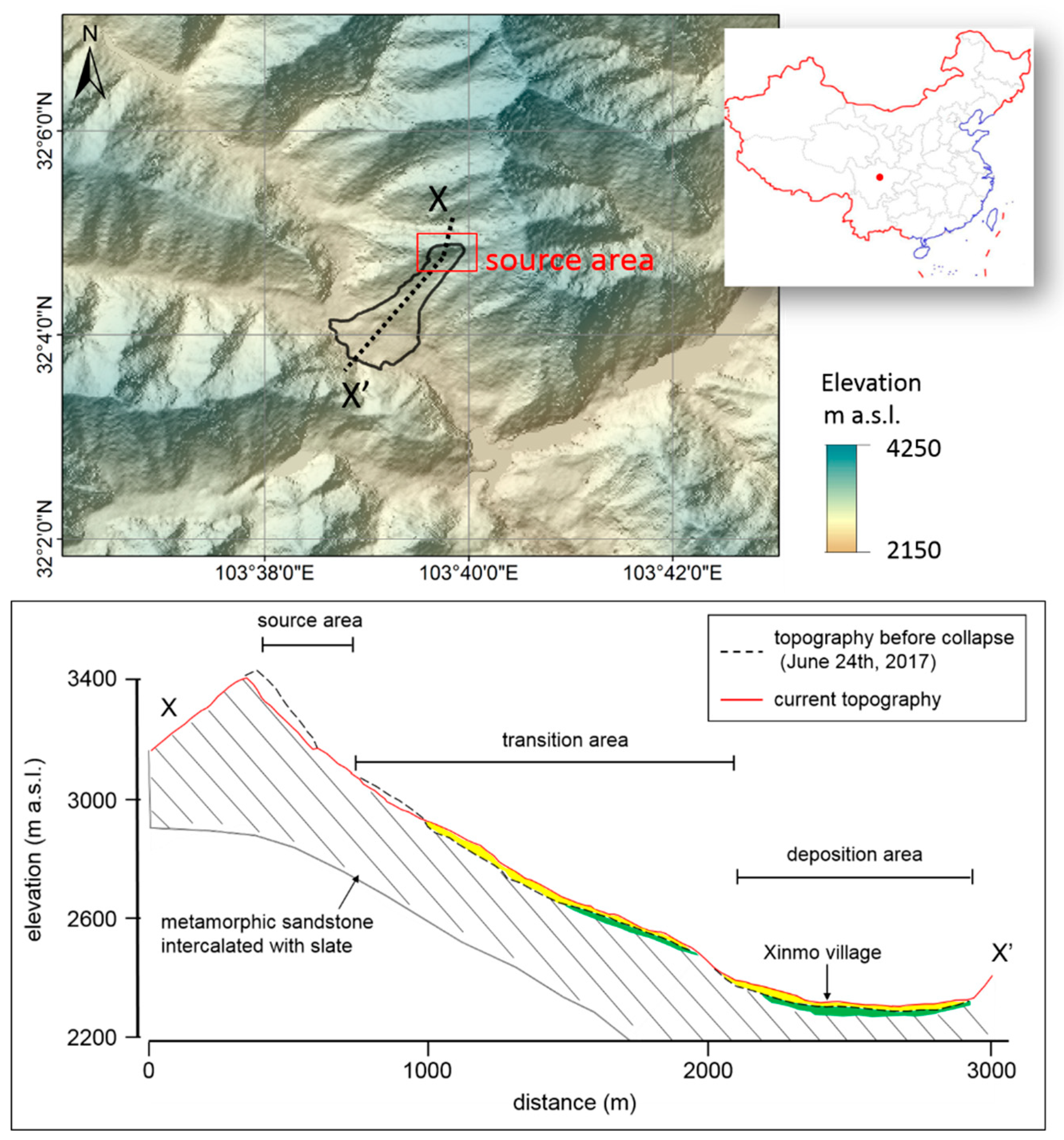
Figure 1. (Upper) The digital elevation model (DEM) of the study area, where the black outline represents the affected region. The red rectangle shows the location of the source area. (Lower) The geological cross-section of the landslide, in which the yellow represents the deposition caused by the 2017 Xinmo landslide, and the green represents the deposition of an old historical landslide (based on Fan et al. [1] and Dai et al. [15]).
Remotesensing 11 01846 g001
Figure 2. The configurations of the temporal and spatial baselines of interferograms: (a) Envisat data, (b) Sentinel-1A/B data.
Remotesensing 11 01846 g002
Figure 3. (a) Average line of sight (LOS) deformation rate from Sentinel-1 (9 October 2014–19 June 2017). The white line represents the failure boundary of the landslide in all panels. (b) Average LOS deformation rate from Envisat (16 June 2008–26 July 2010). (c) Standard deviation of the phase rate from the Sentinel-1 interferograms. (d) Standard deviation of the phase rate from the Envisat interferograms. The time–series deformation measurements in the rectangular regions S1, S2, S3 and S4 were extracted for further analysis in Section 4.1 and Section 4.3. (e) Google-earth image of the landslide. PP’ was along the average downslope direction. The dashed lines AB, CD and EF denote the profile locations.
Remotesensing 11 01846 g003
Figure 4. The cross-sections of downslope deformation rate and the landslide elevation. The locations of (a) cross-section AB, (b) cross-section CD and (c) cross-section EF are shown in Figure 3e. The red triangle and blue circle represent the result from the Sentinel-1 (9 October 2014–19 June 2017) and Envisat (16 June 2008–26 July 2010), respectively.
Remotesensing 11 01846 g004
Figure 5. The time–series cumulative deformation in the line of sight (LOS) direction in the S1 region and precipitation in Xinmo village. The blue circles show the cumulative deformation, and the red squares show the deformation rate. The shaded orange region is the stage of acceleration, the red dash line represents the starting point of acceleration, and the red vertical line represents the time of collapse. The rainfall data (0.1-degree spatial resolution and one-day temporal resolution) was obtained by the Global Precipitation Measurement (GPM) (downloaded from: https://pmm.nasa.gov/data-access/downloads/gpm [30]).
Remotesensing 11 01846 g005
Figure 6. (a) Deformation rate along the down slope direction; (b) modeled down-slope deformation rate; (c) residuals between the observation and the model; (d) observed versus modeled slip rates along profile PP’ shown in Figure 3e. (e) Landslide inversion model, in which the red rectangle represents the dislocation model used to estimate the thickness and slip distribution of the landslide.
Remotesensing 11 01846 g006
Figure 7. Slip distribution at the landslide basal plane, in which the arrows inside each block represents the direction of the shear movement. The bold black line represents the failure boundary of the landslide, and the finer black dotted line represents the boundary of the area with obvious terrain change. The red dashed lines represent the locked section (based on Wang et al. [5]).
Remotesensing 11 01846 g007
Figure 8. Downslope deformation rate and its gradient along the downslope direction PP’; the location of the rectangular profile is shown in the Figure 3e.
Remotesensing 11 01846 g008
Figure 9. The time series deformation from Sentinel-1 data in the LOS direction. The reference time for cumulative deformation begins 9 October 2014. The entire time series deformation is shown in Figure S1.
Remotesensing 11 01846 g009
Figure 10. Time series deformation of the S2, S3 and S4 regions from Envisat data (upper panel) and Sentinel-1 data (lower panel). The extents of S2, S3 and S4 regions are shown in Figure 3d.
Remotesensing 11 01846 g010
Figure 11. A simplified diagram of the expansion of the slip surface. The red line represents the sliding surface of the source area. Referring to Wang et al. 2018, the position of the locked section is located as shown.
Remotesensing 11 01846 g011