The Depths of Cast Shadow

Abstract

To improve the accuracy of analysis outputs from remotely sensed images, shadow and illumination effects need to be minimised or removed. Shadow behaviour at different spectral wavelengths needs to be understood to quantify shadow accurately. This study examined whether a normalised spectral signature of shadow is invariant to sun–object–sensor geometry and can be used to quantify shadow depth. A “FieldSpec® Pro FR” Spectroradiometer and a Canon 450D digital SLR camera were used to measure signatures of cast shadow. Our field-based experiment used an occulter to cast shadow onto a ‘Spectralon’ white plate at six incremental zenith angles and evaluated shadow behaviour within and between varying footprints. A white-balanced image of each shadow zenith was taken by the Canon 450D. The FR Spectroradiometer signatures were normalised to unit vector form and compared to longitudinal transect profiles of shadow from normalised camera images using a scattering index (SI). The normalised signatures show that shadow depth is darker and more ‘blue’ at the proximal areas and conversely that image brightness values increases towards distal areas. Since image brightness is a result of sun–object–sensor geometry, we conclude that a normalised spectral signature is invariant to geometry and can be used to quantify shadow depth.

1. Introduction

Remotely sensed optical images of the Earth’s surface capture information as raster-based images with one or more wavelength bands. Since the Earth’s surface is illuminated by the sun, the geometry of sun location and sensor location at the time of image capture determines the degree of illumination and shadow effects within an image [1,2,3]. Additionally, illumination and shadow effects are further complicated by surface terrain, atmospheric effects, and the physical/chemical characteristics of surface materials that absorb, transmit, or reflect light energy in varying quantities [2].

Detection and removal of these illumination and shadow effects is critical for accurate image analysis and classification because their presence skews image pixel values [4]. De-shadowing in remote sensing is the recovery of a material’s response from within shadow-affected areas of the imagery. Within dark shadow pixels there remains a small signal from the surface material and successful de-shadowing first requires quantification of shadow from within a shadow-affected pixel [5,6,7]. Effective de-shadowing techniques in remote sensing use complex physics-based algorithms that consider sun–object–sensor geometry, BRDF, terrain, and atmospheric correction procedures [8]. With the advent of increasing spatial resolutions of spaceborne, airborne, and drone sensors, the resultant increase in image detail and complexity can cause exponential increases in the complexity of physics-based de-shadowing approaches. Ideally, de-shadowing techniques that are less reliant upon complex physics-based correction procedures can provide more efficient and less complex methods for removing shadow effects to improve image classification and analysis [7].

Shadow effects are a result of illumination variations so it is a prerequisite to characterise illumination effects before shadow detection and quantification is possible [5,7,9]. Illumination conditions for remotely sensed images can be quantified at the time of image acquisition from the atmospheric conditions at the geographical location of the target and the sun–object–sensor geometry. Conversely, an examination of shadow properties can characterise illumination conditions, so a brief review of shadow definition follows.

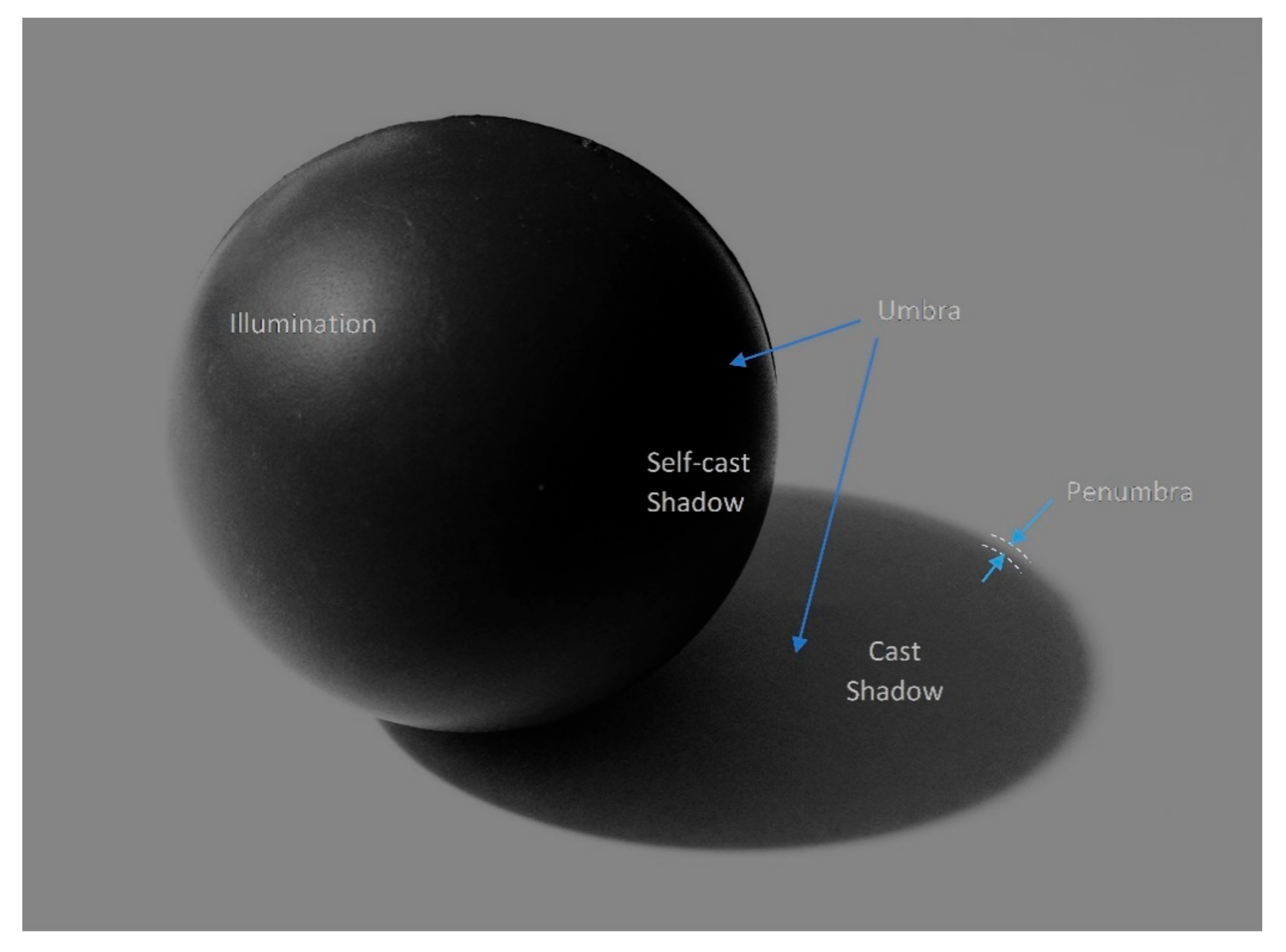
The physics, properties, and classification of shadow are detailed in the works of Funka-Lea and Bajcsy [10] and Arévalo et al. [11]. Shadow is categorised into either cast or self-cast shadow, as shown in Figure 1.

Cast shadow is where an object projects a shadow onto another object so that free space exists between the two objects. Self-cast shadow is where an object casts shadow onto itself because of its morphology or sun–object–sensor geometry. Furthermore, shadow itself is classified into umbra and penumbra regions. Umbra regions are where there is no direct solar illumination and penumbra is the transition region between umbra and non-shadowed areas where light rays are partially obstructed [10,12]. Most shadows are predominantly umbra whereas the penumbra is a narrow transition zone at shadow edges [12].

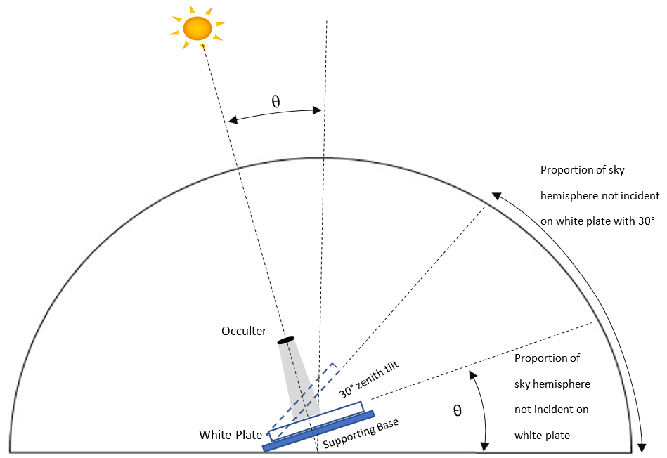
A thorough study of shadows by Lynch [13] examined their theoretical properties and compared them to field-based results from shadows generated by a black circular occulter. The study theoretically modelled shadow illumination and brightness by hemispherical integration of sky radiance, sun radiance, and upward-pointing solid angles subtended by the occulter. Lynch [13] demonstrated that shadows are a 3D volumetric phenomenon influenced by sun zenith and sky radiance. The field-based design suspended a black circular occulter at various heights to cast shadow onto a diffuse white horizontal surface. Comparison of theoretical and field-based results showed that brightness within any part of a shadow cast by a black circular occulter is proportional to the amount of hemispherical sky radiance visible from that part of the shadow. The proportion is calculated using subtended solid angles (Ω) with an example of two different angles shown as a 2D representation of a 3D reality in Figure 2.

From Lynch [13], it is shown that variations of sun zenith, occulter width, and height will alter the solid angles subtended into the sky hemisphere. For a circular occulter, lower Sun altitudes will cause a longer and more elliptical shadow shape, whereas variations in occulter width and height will alter shadow size due to the angular width of the Sun.

Using transect profiles across shadow footprints in field-based images, Lynch [13] found that shadow is ‘blue’ i.e., blue is brighter than green, which is brighter than red. Also, cast shadow at Sun zenith 0° was darkest at the centre and became brighter radially outward towards shadow limits. Additionally, transects were measured over three increases of occulter height using a height-to-width ratio. As the occulter height was increased, the central darkening effect became less prominent with blue, green, and red transect signatures being flat at a height/width ratio of 6.5. The brightness distribution was also reinforced with an elliptical shadow cast from a 30° Sun zenith. The proximal edges of shadow where the subtended angle Ω is greatest were darker than the brighter distal edge where Ω is smallest.

Images used by Lynch [13] were not calibrated to true relative intensity. This is evident from transect results where the white diffuse background response of the transect do not contain equal values of Red, Green and Blue (RGB) signals. Lynch [13] also highlights the complexity of geometric calculations to compute brightness distribution across a shadow footprint when Sun zenith, occulter height, and size factors all combine to create variable oblique shadow footprints. As such, any design for a field-based study of this type should maximise the control of these geometric variables to isolate results to a single variable.

Following the examination of Lynch [13] we assess the colour and depth of cast shadow onto a reference white plate panel with incremental sun–object–sensor angles. Cameron and Kumar [7] use a diffuse skylight vector as a surrogate for shadow depth and this study adopts that methodology. The diffuse skylight is represented as a unit vector and the quantity of diffuse skylight (shadow) in each pixel is determined by the scattering index (SI) that is derived from vector projection using linear algebra. In their study, Cameron and Kumar [7] conducted a comparative evaluation of their SI technique against the first valley thresholding method of Nagao [14] and the SMACC (sequential maximum angle convex cone) endmember extraction algorithm of Gruninger et al. [15]. The comparison specifically targeted areas of known shadow anomalies within high-resolution ADS40 (50 cm) and Worldview-3 (1.2 m) images. The SI proved superior with an overall accuracy of 79% compared to that of 63.3% and 55.6% for Nagao and SMACC, respectively.

The SI approach can compare the response of both shadow colour and shadow brightness under varying sun–object–sensor geometries. Also, we can accurately quantify shadow colour and depth by obtaining the spectral signature difference between a shadowed and non-shadowed reference. With these tests, the authors examine the hypothesis that a normalised spectral signature of shadow colour is invariant to brightness effects associated with sun–object–sensor geometry and can be used to quantify shadow depth. To overcome the complexities of geometry and the resulting variance would be valuable for high-resolution image analysis methods because it removes the need for commensurately scaled data such as terrain and BRDF (bi-direction reflectance distribution function) models [16,17]. A simplified and less scene-dependent approach to quantifying shadow depth and extent has vast potential to benefit many remote sensing applications because it would provide the data for de-shadowing that achieves improved classification and analysis of high spatial resolution imagery. For example, such an approach would enable shadow detection in complex higher-resolution images of urban environments without using commensurately complex 3D models and algorithms. Another example is that of higher-resolution images of vegetation or forest scenes that contain complex levels of morphological variability and spectral heterogeneity. Shadow detection approaches that overcome reliance upon scene-dependent or sensor-dependent characteristics will overcome those increased exponential complexities inherent in higher-resolution scenes. Thus, this study begins research into shadow quantification that isolate the effects of shadow so that we may examine shadow independent of the variances associated with sun–object–sensor geometries and of surface material properties.

The study is not a method comparison, so the results and evaluation can only be presented using data from the study. The data processing and analysis for has been implemented using Python code, IDL code, and Research Systems, Inc. ENVI software.

2. Materials and Methods

The method was an outdoor study that captured reflectance signatures from varying depths of shadow under clear sky conditions. For six incremental shadow depths, a reflectance signature was captured by a field-based spectrometer and a Canon 450D digital camera captured a concurrent RGB image in RAW format.

2.1. Experimental Design

Shadow was created by a suspended black felt occulter disk that projected its shadow footprint onto a 300 mm square Spectralon white panel, hereafter referred to as the ‘reference panel’. To simulate varying depths of shadow, the reference panel was tilted towards the sun in six 10° increments from 0° to 50°. In the design, azimuth increments were not tested for two reasons; it complicated the design and cast shadow depth variation is more accurate with only one changing variable i.e., zenith. The outdoor design and analysis process is summarised stepwise below.

• Orientate the white plate normal to the Sun (0° zenith) and record six hyperspectral reflectance signatures and one high-resolution RGB image. Six signatures were collected at random locations across the plate and averaged to obtain a reflectance signature for the white plate.
• The black felt occulter was suspended horizontally above the white plate to create a cast shadow onto the plate.
• Cast shadow depth and shape were altered by simulating six different zenith angles that are created by tilting the white plate to 0°, 10°, 20°, 30°, 40°, and 50° zeniths.
• At each zenith angle, six hyperspectral reflectance signatures were recorded and were equally spaced longitudinally from proximal (dark) to distal (light) shadow within the cast shadow footprint. Reflectance signatures of blue sky were captured by pointing spectrometer upwards into clear sky areas. The signatures were used to quantify the amount of diffuse skylight scattering.
• A Canon 450D camera was used to capture one high-resolution RGB image in Canon RAW (.CR2) format for every zenith angle.
• The spectrometer’s reflectance signatures were analysed and compared using the SI of [7]. in each Canon photo captured, a longitudinal transect through the shadow was created to graphically compare the difference in shadow brightness and colour between zenith angles.

These steps are discussed in more detail below followed by specifications of the spectrometer and Canon 450D Camera. Figure 3 graphically details the design of the experiment from steps 1–4 above.

For each reference panel zenith angle, six spectral signature samples were taken equidistant along the longitudinal spread of the cast shadow footprint at a height of 150 mm above the reference panel. As shown in Figure 3, signatures are numbered 1 to 6 from proximal shadow (dark) to distal (light) shadow, respectively. A single Canon EOS 450D image is taken for each material at each zenith angle whereby the view angle is normal to the reference panel and the camera was 1 m above the reference panel and 1 m horizontally from the shadow centre.

From Figure 3 it can be observed that there are two variables that change. One variable is the required treatment for our experiment, the reference panel zenith changes to simulate shadow shape and depth. The other variable is the amount of solid angle sky hemisphere Ω incident on the shadow with each zenith change. Figure 4 highlights this by showing that adjustment of the supporting base to be normal to the Sun reduces the sky hemisphere incident on the reference panel. It also shows that a further 30° zenith tilt of the reference panel reduces that sky hemisphere even further. It is important to highlight this because sky hemisphere exposure is fundamental to the brightness hypothesis of Lynch [13]. However, pre-processing calibrations to the spectrometer and Canon 450D negate this effect and are discussed in the Sensors section further below.

2.2. FR Spectroradiometer

The spectrometer used was an ASD “FieldSpec® Pro FR” FR spectroradiometer (Analytical Spectral Devices, Boulder, CO) with a spectral range of 350–2500 nm and a 1 nm sampling interval. The capture of signatures is done via a hand-held pistol that is connected to the FR spectroradiometer via a fibre optics cable. The hand-held pistol can be fitted with foreoptic lens attachments that have varying field of views (FOV). For this study, a foreoptic lens with a 3° FOV was fitted to the pistol. The FR spectroradiometer is calibrated to capture reflectance using reference panel with approximately 100% reflectance across all spectra. The reference panel is a near-perfect ‘white body’ that provides a baseline to calibrate the sensor and capture real time relative reflectance.

The spectrometer signatures and Canon 450D images were captured on a cloudless day at Woolgoolga, NSW, Australia. The experiment was conducted on an open flat sporting field over two hours between 12:00 and 14:00 with sky visibility down to 10° altitude or less. Sun zenith/azimuth at 12:00 and 14:00 was 55°51′/356°15′ and 44°06′/312°25′, respectively. These times were selected to maximise the highest Sun zenith angles and to reduce the amount of frame adjustment. Figure 5 shows the field setup for the spectrometer using a metal wire crate as the frame, black plywood for supporting base, brown plywood for tilt plate, and a nail for the zenith/azimuth post. The tilt plate has been hinged to the supporting base to ensure linear tilting and a sliding square tube guide with increment marks is used to ensure equal spaced signature capture with the pistol across the shadow footprint.

Prior to shadow signature capture at each zenith iteration, the FR Spectroradiometer was optimised and dark current corrected to reflectance in situ using a non-shadowed portion of the reference panel. The foreoptic lens targeted a non-shadowed portion of the panel that was sighted using the pistol slide guide. At a pistol height of 300 mm, the 3° FOV foreoptic lens captures an approximate circular footprint of 15.7 mm diameter on the reference panel, thus leaving adequate panel space to optimise. The optimisation and subsequent six shadow signatures at each zenith took less than 10 min, minimising any changes in atmospheric effects between sample and target i.e., 10 min equates to 0.3° sun zenith change. The reflectance calculation is the ratio of the shadow signature to the optimised reference panel signature, thus minimising atmospheric and illumination effects such as any irradiance obstruction from the operator, wire crate, occulter, instruments, and the sky hemisphere reductions shown in Figure 4. Estimates of measurement uncertainties in the design result from illumination variation, illumination variance caused by nearby objects, geometry of the design, Spectralon panel degradation, and the Lambertian scatter properties of the Spectralon panel [18,19,20,21]. Estimations of these measurement uncertainties by these factors are provided in the Discussion.

For the reference panel reference signature with no shadow, the spectrometer hand-held pistol captured six spectral signatures taken at six randomly selected locations across its surface. The signatures are then averaged to obtain the reflectance signature for reference panel. For the sky signature, the pistol was detached and pointed upwards towards the clear sky to capture signatures. Two separate upward directions were used, one at 45° azimuth and 30° zenith and the other at 0° azimuth and 0° zenith. Six signatures were taken at each direction and all 12 were averaged to produce a final reflectance signature. All signatures were post-processed to remove high-frequency noise by using a moving average filter with boxcar size 15.

2.3. Canon 450D

A digital Canon EOS 450D camera was used to capture RGB images of shadow at each reference panel zenith angle. The Canon EOS 450D has an APS-C CMOS (active pixel sensor–complementary metal oxide semiconductor) sensor that captures high-resolution images in raw or CR2 format. Wavelengths of Canon camera sensors are difficult to ascertain but wavelengths for the EOS 450D can be directly translated from the Canon EOS 400D, which has the same sensor. Schläpfer et al. [22] calculate the band maxima for RGB wavelengths for the Canon EOS 400D and, thus, the EOS 450D, as shown in

Table 1. Canon EOS 400 and 450D sensor wavelengths. Band maxima for red, green, and blue.

Band	Wavelength (nm)
Blue	450
Green	540
Red	600

.

The Canon camera was prepared for image capture by manually setting the white balance from a photo of the reference panel, which is equivalent to a conversion to reflectance. The initial reference photo of the reference panel will not have exactly equal RGB values because of camera settings, atmospheric absorption, and illumination effects. However, three scaling factors can be formulated from that image and then applied to each band to ensure the RGB values are equal and, thus, calibrated to the reference panel as reflectance. Importantly, using this white balance, we can characterise the photos as reflectance equivalent because of the reference panel; any other ‘white’ surface material would not be a near perfect ‘whitebody’. White balance correction on the Canon 450D was performed before every reference panel zenith change. Again, this image correction to a ’pseudo’ reflectance negates the sky hemisphere effects shown in Figure 4.

Figure 6 shows the setup for the Canon 450D image capture. This is the same setup as Figure 5 except an alternative open frame (separate to the wire crate) was used to allow unhindered visual access to the shadow. At each zenith, the supporting base with tilt plate, zenith/azimuth post, and reference panel attached was relocated from wire crate setup to the open frame for Canon 450D image capture. The frame has four aluminium corner posts that were used to suspend the occulter by connecting four diagonal black cotton lines connected to elastic bands at the corner posts to maintain tension. The four posts were incrementally marked in 20 mm gradations so that the four cotton-elastic suspender lines could be lifted up or down to keep the occulter horizontal and with constant height of 300 mm above shadow centre.

Canon images are imported into ENVI software and pre-processed to remove high-frequency noise using a 11 × 11 median filter.

2.4. Analysis

To test that unit vector normalisation (colour) of a reflectance signature is invariant to the brightness effects of sun–object–sensor geometry, the correct range of wavelengths are important. For the FR Spectroradiometer, spectral reflectance signatures are captured for wavelengths in 1 nm sampling intervals from 350–2500 nm and exported as comma separated value (CSV) files. However, the study focus is confined to the visible wavelength range of 400–700 nm. This is because most optical sensors capture wavelengths from 400 nm and above and 700 nm is the upper limit for the visible spectrum [23,24].

The reflectance signatures from the cast shadow on the reference panel normal to the Sun (0° zenith) are used to determine the upper wavelength limit where the diffuse skylight effect ceases. The FR Spectroradiometer shadow signatures will be analysed for the mean of their lowest values within the 400–700 nm range. Shadow signatures are characteristically defined by the diffuse skylight effect that is an exponential decay function [5,6,7]. So, to remove potential error we buffer the upper limit range to 800 nm and use the lowest reflectance value within 400–800 nm range to mark the upper wavelength limit S_max of the exponential decay effect.

For both FR Spectroradiometer and Canon 450D responses, the analysis uses the SI to compare shadow depths, so a measure of the diffuse skylight scattering effect is required to generate our reference scatter vectors [7].

The skylight measure is obtained by a non-linear least squares curve fitting of the relative scattering model λ^−x to the averaged skylight signature captured by the FR spectroradiometer. The curve fit function is applied in the Python SciPy model (scipy.optimise.curvefit) using the Levenberg–Marquardt fitting model [25]. The curve-fitting result will provide the best fit Angstrom-law exponent x for the relative scattering model λ^−x to generate a scatter vector that matches the experiment conditions. Using Equation (1), we convert the reference scatter vector to unit form but instead of using the 400–700 nm wavelength range, we adopt the upper wavelength limit of S_max mentioned previously

$$\widehat{S}= \frac{{\mathit{\lambda }}_i{}^{-x}}{\sqrt{{\sum }_{\mathit{i}=1}^{\mathit{n}}{\left({\mathit{\lambda }}_{\mathit{i}}{}^{-x}\right)}^2}}$$

(1)

where $\widehat{S}$ is the unit scatter vector, $x$ is the Angstrom-law exponent, λ = wavelength, and n the total number of wavelengths from 400 nm - S_max.

The shadow signatures generated from the FR Spectroradiometer are restricted to the 400 - S_max wavelength range then converted to unit vector form using Equation (2)

$$\widehat{\mathit{p}}= \frac{p_i}{\sqrt{{\sum }_{i=0}^n{p}_i^2}}$$

(2)

where $\widehat{\mathit{p}}$ is unit vector, ${\mathit{p}}_{\mathit{i}}$ is reflectance value at wavelength i, the number of wavelengths is n, and the denominator term is the magnitude of the signature in vector form. Unit vector magnitude $\left|\left|\widehat{\mathit{p}}\right|\right|$ is always 1.

SI values are calculated for each signature at each zenith angle using the dot product from $\widehat{\mathit{S}}$ and $\widehat{\mathit{p}}$ as per Equation (3)

$$SI= \widehat{\mathit{S}}·\widehat{\mathit{p}}.$$

(3)

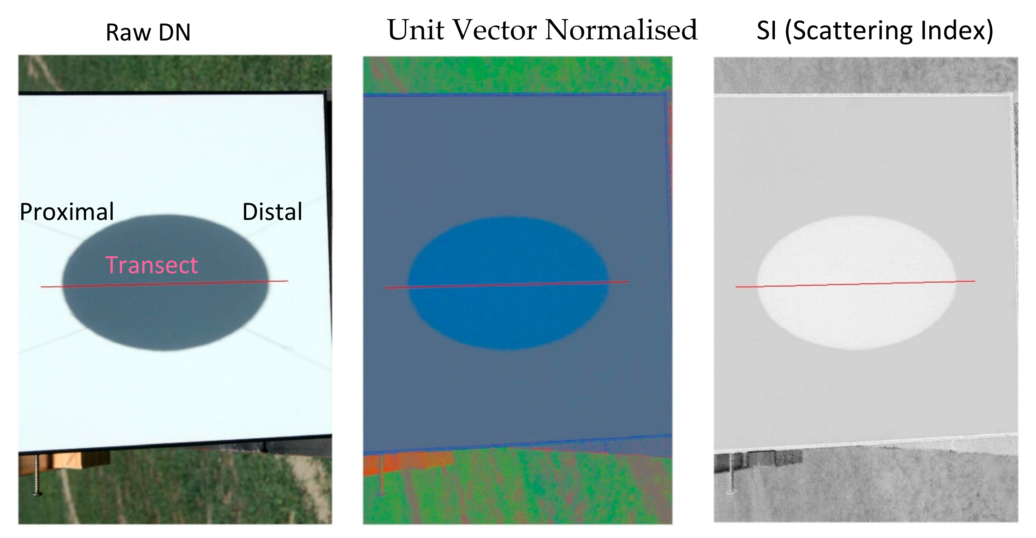
The responses of shadow colour and brightness are measured from the Canon 450D images of shadow. The broad integrated response from the three-band Canon 450D sensor cannot be accurately matched to the precise one nanometre signatures of the FR Spectroradiometer. This is addressed in the analysis by using a common transect across the shadow footprint for both sensors. For each zenith image captured by the Canon 450D, a longitudinal transect is generated across the shadow from dark to light shadow depth as per the spectrometer signatures. The FR Spectroradiometer captures separate hyperspectral signatures per shadow footprint whereby each signature measures the varying depth of shadow. Alternatively, the Canon 450D captures the same varying depth of shadow by a single and continuous three-band signature profile per transect. Transects are presented graphically with the transect beginning and ending on the outside of the shadow in the reference panel area to quantify the shadow effect. A transect example is shown in Figure 7.

Each image will graphically plot three versions of the transect. First is the raw Digital Number (DN) of RGB bands, the second is the RGB bands in normalised unit vector form using Equation (2), and the third is a graph of the SI index. The SI for the Canon 450D is generated to match the RGB bands of the camera. Therefore, the diffuse scatter vector will be calculated from its three bands (450, 540, and 600 nm) using Equation (1) with the Angstrom-law exponent that results from the curve-fitting.

Also, from a wavelength range of 400 to 1000 nm we create a grey vector i.e., all wavelengths are equal. The grey vector is a theoretical black/grey/white body reference that is colourless and aids as an independent reference for the degree of colour for all other vectors. The grey vector is converted to unit vector form by a simplified form of Equation (2).

$$\widehat{\mathit{g}}= \frac{1}{\sqrt{n}}$$

(4)

where $\widehat{\mathit{g}}$ is the grey vector unit value for number of wavelengths n. Again, unit vector magnitude $\left|\left|\widehat{\mathit{g}}\right|\right|$ is always 1.

Importantly, the reflectance signature of the non-shadowed reference panel should equate to the grey vector, so a simple statistical comparison is provided at the end of the results section below.

3. Results

The reflectance signatures from each of the six zenith angles have the SI values calculated using a reference scatter vector derived from the ${\mathit{\lambda }}^{-2.6945}$ relative scattering model shown further below in Figure 13. Figure 8 shows the SI values for each signature with the grey vector and scatter vector displayed for reference. In each of the Figure 8 plates, the legends show Sig. 1 through to Sig. 6 vertically and this is from proximal to distal shadow, respectively.

From Figure 8 there are trends in shadow colour from 0–50 degrees zenith. As zenith angle increases, there are four observable trends; a) overall SI values decrease, b) the difference in SI value between proximal (darker) shadow and distal (light) shadow increases, c) proximal areas of shadow have higher SI values than distal areas of shadow, and d) the end of the exponential decay effect of diffuse scattering shifts towards smaller wavelengths. For example, at 0° zenith, the skylight effect ends at 675 nm whereas for the 50° zenith in Plate (f), the skylight effect ends at approximately 500 nm where signatures are at their lowest. Figure 9 plots the SI values of signatures at each zenith and highlights the trends mentioned above.

All plates in Figure 8 show a convergence point at approximately 520 nm where the scatter vector and shadow signatures are equal. For wavelengths from 400 nm–520 nm, Sig. 1 has a higher SI value than Sig. 6 and the reverse occurs from the 520 nm–675 nm wavelength range. This is more evident in the 30°, 40°, and 50° zenith plates. From Equations (1) and (4), we know the intersection of the scatter vector and grey vector is calculated at exactly 500 nm and appears correlated to the convergence point.

The diffuse skylight vector for the three-band Canon 450D images is calculated from the Angstrom-law exponent –2.6549 (Figure 13) substituted into Equation (1). The scatter vector is in unit form and shown in

Table 2. Diffuse skylight scatter vector calculated from Angstrom-law exponent –2.6549 for Canon 450D sensor.

Band	Wavelength (nm)	Scatter Vector (unit vector)
Blue	460	0.79
Green	540	0.51
Red	620	0.35

.

As the Canon images are already pre-processed to ‘pseudo’ reflectance, they are directly converted to unit vector form and the SI is generated for each image by the dot product of the unit vector image and the unit scatter vector. Figure 10 is an example of the process using the 50° zenith shadow images and the three images used to derive three transect graphs (raw DN, unit vector, and SI) per zenith angle. Figure 11 displays the graphical results for all six zenith angles.

The Canon image results mimic the trends to that of the FR Spectroradiometer. However, the Canon sensor’s inferior sensitivity and spectral range/resolution combined with 10° zenith increments, a 300 mm shadow height, and relatively small occulter all result in data with reduced discrimination. To overcome and assist with interpretation of the reduction, a smaller shadow-only reference transect is included for the raw DN, unit vector, and SI graphs.

In the raw DN transects, the shadow-only reference is the minimum red value that highlights two trends linked to increasing zenith angle. One is that overall DN values increase i.e., a 0° zenith DN of 69.8 climbs to 91.8 at the 50° zenith. Secondly, DN values at the distal end of shadow become higher than those at the proximal end.

In the unit vector transects, the reference panel responses at the extremes of the transects match the grey vector and this reinforces the white balance pre-processing of the Canon images. These transects also show the strong blue response of shadow when pixel magnitude is normalised. Again, two trends are linked to increasing zenith angle. One is that shadows responses reduce towards the grey vector and the second is that the distal ends reduce faster than the proximal ends. In the SI transects, the shadow-only reference is the maximum SI value and it reinforces the trends noted above. As zenith angle increases, the overall SI values get smaller and the distal ends reduce more than the proximal ends. The other important trend is that with smaller zenith angles, the difference between proximal and distal responses reduce to become almost flat at 0° zenith.

The diffuse skylight effect for the experiment shows that for a shadow cast by an occulter at 0° zenith and azimuth the exponential decay behaviour ceases at 674.16 nm. Figure 12 highlights this graphically with the mean of minimum values from the six reflectance signatures that were collected from spatially random locations within the shadow footprint. The diffuse skylight upper limit is rounded to 675 nm and used as the upper wavelength range in all analysis results.

From the spectral signatures captured by pointing the FR Spectroradiometer at the sky, we calculate the mean signature and restrict its wavelength range from 400 nm to 675 nm. Figure 13 displays the non-linear least squares curve-fitting resulting in an Angstrom-law exponent of –2.6945 as the best fit for the mean skylight signature supported by a Pearson correlation coefficient of p = –0.969.

The reflectance signature of the reference panel from the FR Spectroradiometer is highly correlated to a theoretical grey vector. From the six spectral signatures of the reference panel, the mean was calculated then restricted to a wavelength range of 400 to 1000 nm. The mean signature was then normalised to unit vector form. The theoretical grey vector was created from the same wavelength range (n = 601) using Equation ((4) resulting in a unit vector value of approximately 0.040791. Statistics from the comparison of the two are shown in

Table 3. Statistical comparison of normalised reflectance signatures from the reference panel and a normalised theoretical grey vector. Mean reflectance is the mean of all reflectance values between 400–1000 nm.

Signature (unit vector)	Mean Reflectance	Standard Deviation
Reference panel	0.0407908508224004	1.873 × 10−16
Grey Vector	0.0407908508224002	n/a

and demonstrate an almost identical match with the difference only beginning at a 16th decimal precision shown by the mean reflectance column.

4. Discussion

Results show that a normalised measure of shadow is invariant to the brightness effects associated with sun–object–sensor geometry and provides a measure of colour depth. The results are supported by data from a high-precision FR Spectroradiometer and white-balanced images from a Canon 450D camera. When the FR Spectroradiometer reflectance signatures are normalised to unit vector form, we are afforded an independent physics-based reference in the grey vector [7]. The unit vector transformation of pixels and the grey vector provide an invariant shadow measure because all vector magnitudes are 1 and the count of wavelengths or axis is independent of the actual data values. Conversely, traditional normalisation of a data series uses the upper and lower bounds of the series data values to rescale; it does not use the count of samples. Standardisation of a data series is based upon the mean of that series and the mean is a non-independent reference. At this base level of review, any comparison between two or more series using normalisation or standardisation will be based upon uncommon references. Unit vector transformation provides the independence and the grey vector is the physics-based model of a theoretical white-black material. Cameron and Kumar [7] show that inverse cosine conversion of unit vector values results in angular distance and, thus, shadow vectors can be quantified by their angular distance from a diffuse skylight scatter vector. The angular distance between the skylight vector and grey vector provides a reference for shadow extent. This is demonstrated in Figure 8 and Figure 11 where the unit vector signatures are measured against the grey vector and the diffuse skylight vector. Without normalisation, the data from the Canon image transects in Figure 11 do show that brightness response is proportional to the amount of sky hemisphere irradiance as supported by Lynch [13]. However, using the minimum red value transect from Figure 11 as an example, the raw DN values range from 69.8 at 0° zenith to 91.8 at 50° zenith. The data do reflect expected trends of shadow response but comparison with data from another sensor is difficult because of varying sensor characteristics such as the conversion of radiant energy to DN, sensor calibrations, radiometric range, spectral range, spectral resolution, and image pre-processing method. So, conversion of data to unit vector form provides invariant shadow metrics because data can be measured against independent physics-based references i.e., the diffuse skylight and grey vectors. These references are invariant to the brightness effects associated with sun–object–sensor geometry.

There is a requirement to define shadow and its ‘depth’ before it can be measured. Shadow is a result of illumination characteristics where direct solar irradiance of a target is obstructed and the volume of sky that is left above the target becomes the source of illumination [5,13,26]. Since shadow response is directly related to diffuse skylight, we know that shadow appears as a ‘blue’ colour, which is a convenient definition. The definition is more scientifically defined by the exponential decay function ${\mathit{\lambda }}^{-x}$ shown by the FR Spectroradiometer signal of the sky in Figure 13. The effect is prominent within the visible domain where shorter wavelengths reflect exponentially more than longer wavelengths. For purposes of the discussion, Figure 14 highlights this effect when the FR Spectroradiometer sky signature is extended to a 350–1000 nm range. It can also be observed from Figure 14 that the nature of an exponential decay function does not entirely flatten out and never will. However, the increasingly smaller scattering influences at longer wavelengths may be of significance to hyperspectral data applications such as mineral classification where subtle changes in signatures could be critical.

The results from the Canon image transects in Figure 11 reflect this effect because with increasing zenith there is more skylight irradiated onto the target and the DN values rise commensurately i.e., from 69.8 to 91.8. However, from the same unit vector and SI transects in Figure 11, we see an inverse effect where increasing zenith causes unit vector values to reduce towards the grey vector and the SI reduces overall i.e., from SI value 0.991 to 0.978. This is reinforced by the FR spectrometer data in Figure 9. where the SI reduces from approximately 0.98 to 0.925. The inverse effect of the SI is only due to the unit vector transformation and the skylight effect is reinforced by all data. It is important to note here that the difference in the SI value ranges 0.991–0.978 and 0.98–0.925 are a direct result of the FR Spectroradiometer’s superior sensitivity, spectral resolution, and range. Shadow depth should be defined by similarity to diffuse skylight as per the SI. The spectral signatures in Figure 8 reinforce this because the SI increases with darker proximal shadow where there is a larger solid angle subtended. This is counter-intuitive to the findings of Lynch [13] where shadow ‘blueness’ increases in distal parts of shadow because of the smaller solid angles subtended. In terms of ‘brightness’, the distal areas appear more ‘blue’ but the removal of magnitude via unit vector normalisation reveals the true depth of the shadow that is darker in the proximal and lighter in the distal. So, similarity to diffuse skylight is the metric to quantify shadow depth because it is invariant to sun–object–sensor geometry, unlike brightness. The only consideration to this approach is the appropriate Angstrom-law exponent to define the skylight effect. The exponent will vary depending on conditions such as geographical location, atmosphere constituency, seasonal variation, Sun zenith/azimuth, sensor height, and spectral characteristics of the sensor.

For the experimental design, it is necessary to estimate FR Spectroradiometer measurement uncertainties that were mentioned previously in the Materials and Methods section. Protocols and procedures (standards) for measurement uncertainty in field spectroscopy is currently a developing discipline and many factors influence the accuracy of target measurements taken by spectrometers [19]. In their thorough examination of uncertainties, Hueni, Damm, Kneubuehler, Schläpfer, and Schaepman [19] highlight issues of cross validation between in situ spectroscopy data and airborne spectroscopy data. This study negates many of the cross-validation uncertainties detailed in their examination since our reference and target are the same i.e., the reference panel. The remaining uncertainties include the following: Variations in illumination (due to solar zenith, nearby objects, and atmospheric scattering), Spectralon panel degradation, reference-to-target measurement timing, and temperature of FR Spectroradiometer instrument. This study did not include a systematic Type A procedure to measure uncertainties, so estimates of percentage declines in performance for each attribute are provided in

Table 4. Uncertainty measure attributes for the study design including study conditions that induce sources of uncertainty.

Uncertainty Measure	Error Estimate for Study (%)	Sources of Uncertainty
Spectralon Degradation	5	12-year-old Spectralon plate with <100 hours UV exposure time
Spectralon Lambertian scatter	3	0–50° panel tilt range. Optimisation performed with pistol +/−5° normal to panel.
Illumination characteristics	2	Acquisition between 12:00–14:00 under clear stable sky
Solar Zenith effects	2	12:00–14:00 equates to total solar zenith change of 11.45°
Reference-to-Target Time	0.5	Less than 10 min i.e., less than a 0.3° change in solar zenith
SFR Spectroradiometer temperature	0	At least 1 hour on power before operation

based upon the various measurement uncertainties provided in Hueni, Damm, Kneubuehler, Schläpfer, and Schaepman [19], Möller, Nikolaus, and Höpe [18], Deadman, Behnert, Fox, and Griffith [20] and Malthus and MacLellan [21].

The recommendations made by Hueni, Damm, Kneubuehler, Schläpfer, and Schaepman [19] to reduce uncertainty measures (excluding the age of Spectralon panel) have been indirectly achieved by the reproducibility of the study design. Reproducibility was achieved via fixed frames and controlled geometries of all moving parts and instruments [19]. In terms of Lambertian scatter uncertainty, Deadman, Behnert, Fox, and Griffith [20] recorded minimal uncertainty of <0.1% reflectance factor for six reference panels from a 500 nm wavelength at 45°. Their result was conducted under controlled laboratory conditions so our estimate of 3% error for Lambertian scatter is precautionary to cater for external environmental variation. The study reduced illumination variances by minimising times between reference and target samples and maximising highest solar sun angles within two hours of 12:00 [19]. The only variation in illumination was by the pistol and slide guide since the operator was at least 1 m from the design and the wire crate effect was negated by the optimisation. In terms of operation, the FR Spectroradiometer was left running at least one hour before data capture to ensure thermal stability and, thus, eliminate any signal uncertainties incurred by the instrument itself. Overall, the major contributions to uncertainty, albeit a small effect of less than 5%, are the degradation and Lambertian scatter of the Spectralon reference panel. As such, the resultant spectral signatures are largely unaffected by uncertainties that can be controlled. Furthermore, the study uses reflectance signatures that are normalised to unit vector form, further eliminating any bias induced by amplitude variations in radiance or brightness.

The measure of shadow depth can be defined by diffuse skylight but the bounds of that effect are not clear and vary with shadow depth. Avery and Berlin [23] state that the visible wavelength domain of 400–700 nm is accurately defined by limits of human vision but that is not a physics-based range to define diffuse skylight effects. From the FR Spectroradiometer signatures of shadow at 0° zenith in Figure 12, the effect ends clearly at 674.16 nm and we have adopted that as an upper wavelength limit for the study. However, this limit is defined by the conditions of the experiment and is confirmed by closer examination of the signatures in Figure 8. As the zenith increases from 0 °to 50°, the skylight effect ends at progressively shorter wavelengths i.e., a shift from 674.16 nm to approximately 500 nm for the 50° zenith. Additionally, at the higher zeniths of 40° and 50°, it is observed that shadow at wavelengths longer than 560 nm are almost gone because the signatures revert back towards the grey vector. From Table 3 we know that the grey vector is the same as the reference panel so, therefore, we know the shadow is disappearing. The remaining wavelength range of 500–560 nm is still in shadow but displays a positive slope effect and not the exponential decay effect of diffuse skylight. Obviously, these characteristics reflect the transition behaviour of wavelengths from a dark to light shadow and this leads to the last observation not yet discussed from the results. That observation is the convergence of shadow signatures at the 520 nm wavelength that is near the intersection of the grey vector and scatter vector at 500 nm. If we were to visualise an animation of the plates through increasing zenith i.e., Figure 8a–f, two patterns would be observed. One is that the signature progressively flattens and the other is an anti-clockwise rotation about the convergence point. This could be described analogously as someone putting their feet up to lie down and rest from a sitting position. So, if we consider the diffuse skylight effect as exponential decay, then the upper bound of that decay effect contracts towards shorter wavelengths as shadow depth decreases.

A measure of shadow depth that is invariant to sun–object–sensor geometry combined with a knowledge of shadow behaviour provides a model for shadow removal. This study required the near perfect white body plate as an accurate neutral reference to quantify shadow independent of the target material. We, therefore, hypothesise that a shadow removal technique based on these findings would translate to shadow removal from images of realistically occurring materials. This approach may have significant benefits for high-resolution images where scene complexity becomes exponentially more complex in terms of both surface morphology and the number of surface materials detected [7]. For such images, a shadow quantification technique that is independent of scene complexity can negate many of the complex parameters associated with physics-based shadow detection and removal. For physics-based approaches, shadow detection and removal are often integrated into atmospheric correction algorithms [2,6,27]. Furthermore, some of these methods use terrain data and BRDF information to correct illumination and shadow effects. However, for the exponential increases in complexity with higher resolutions, there is commensurate complexity required for data that capture scene terrain/morphology and BRDF information. These complexities are confounded even further in operational circumstances where study areas cover multiple image tiles can be acquired under varying environmental conditions. Therefore, an independent shadow reference can negate many of the complexities required for shadow correction and that results in simplified image pre-processing and analysis techniques for high-resolution imagery.

Here, we find that an independent model for shadow removal is clearly non-linear and requires a shadow depth measure to unmix the effects of diffuse skylight scattering.

5. Conclusions

This study has concluded that a spectral signature of reflectance that is normalised to unit vector form (colour) is invariant to sun–object–sensor geometry and provides the data to quantify shadow and its depth. Unit vector normalisation provides two independent physics-based references for quantification of shadow, the grey vector, and a diffuse skylight vector. A relative scattering model generates the diffuse skylight vector and when combined with the normalised signature of shadow as per the scattering index (SI), it can be used to quantify shadow depth. The darker proximal areas of shadow have higher SI values than the distal areas of shadow and this is an inverse effect to that of measuring shadow by brightness values. Also, when shadow reduces to lower SI values the exponential decay behaviour of diffuse skylight affects an increasingly smaller wavelength range that contracts from longer wavelengths to shorter wavelengths. The findings provide a basis for future research into shadow removal techniques.