A Model-Dependent Method for Monitoring Subtle Changes in Vegetation Height in the Boreal–Alpine Ecotone Using Bi-Temporal, Three Dimensional Point Data from Airborne Laser Scanning

Abstract

The boreal tree line is in many places expected to advance upwards into the mountains due to climate change. This study aimed to develop a general method for estimation of vegetation height change in general, and change in tree height more specifically, for small geographical domains utilizing bi-temporal airborne laser scanner (ALS) data. The domains subject to estimation may subsequently be used to monitor vegetation and tree height change with detailed temporal and geographical resolutions. A method was developed with particular focus on statistically rigorous estimators of uncertainty for change estimates. The method employed model-dependent statistical inference. The method was demonstrated in a 12 ha study site in a boreal–alpine tree line in southeastern Norway, in which 316 trees were measured on the ground in 2006 and 2012 and ALS data were acquired in two temporally coincident campaigns. The trees ranged from 0.11 m to 5.20 m in height. Average growth in height was 0.19 m. Regression models were used to predict and estimate change. By following the area-based approach, predictions were produced for every individual 2 m² population element that tessellated the study area. Two demonstrations of the method are provided in which separate height change estimates were calculated for domains of size 1.5 ha or greater. Differences in height change estimates among such small domains illustrate how change patterns may vary over the landscape. Model-dependent mean square error estimates for the height change estimators that accounted for (1) model parameter uncertainty, (2) residual variance, and (3) residual covariance are provided. Findings suggested that the two latter sources of uncertainty could be ignored in the uncertainty analysis. The proposed estimators are likely to work well for estimation of differences in height change along a gradient of small monitoring units, like the 1.5 ha cells used for demonstration purposes, and thus may potentially be used to monitor tree line migration over time.

1. Introduction

The world’s climate will undergo distinct alterations over the coming decades, leading to rapid changes in basic growth factors, such as temperature and precipitation. This will influence the boreal forest and its transition zones, leading to an increase in productivity [1]. Because the montane and northern forests found in the transition zones between the boreal forest and the alpine and tundra regions appear in areas where trees exist close to their tolerance limit in terms of temperature, these areas are characterized by steep temperature–productivity gradients. Even a moderate increase in temperature may therefore lead to a rapid increase in the growth of existing trees [2,3], as well as colonization of treeless areas and migration of the tree lines [4]. The dynamic global vegetation models predict that by the end of the 21st century, the area of the arctic tundra will be reduced by 40% [5,6]. Other drivers of vegetation change also exist at the forest–tundra interface, like herbivory [7,8,9]. Summer farms and grazing by domestic animals, such as cattle and sheep, have been common in many montane areas. Both the animals themselves and the human activity related to summer farming, such as harvest of wood, have had large impacts on the montane forest and the tree line [7]. In areas where summer farming and grazing animals have previously limited tree growth, the tree line and the montane forest may thus expand towards higher elevations when this activity is reduced. Migration of the alpine and northern tree lines will influence future carbon pools. A need therefore exists to monitor vegetation changes in these ecotones [10].

Acquiring data for monitoring purposes over vast areas is expensive. So far, attempts to simplify ground-based procedures, save costs, and make the monitoring uniform over large areas have relied on remote sensing from space-borne platforms. Satellite remote sensing utilizing optical sensors has been the dominant technology, but data from such sensors have limited capabilities for detecting subtle changes in vegetation over short time periods.

Airborne laser scanning (ALS) has been proposed as a technique to monitor subtle changes near tree lines, such as the colonization of treeless areas [11], and to assist in prediction and estimation of tree height [12,13], tree height growth [13], and biomass [14,15]. Numerous recent studies (e.g., [16,17,18]) have shown that ALS data with point densities of 7–11 points m⁻² may be applied to detect individual pioneer trees in the alpine tree line. With such pulse densities, about 90–100% of the trees with heights greater than 1 m are likely to be hit by laser pulses, resulting in echoes with height values greater than zero, i.e., located above the terrain surface. Echoes with heights >1 m are mainly tree echoes. Rees [19] anticipated that ALS could provide a means for discerning individual trees over hundreds of square kilometers. In that study, a minimum height of 2 m was used as a criterion of a tree.

For trees <1 m in height, positive echo height above the terrain surface is a poor discriminator for discerning individual trees. Using echo height as a predictor for the smallest trees will lead to large commission errors (false positives) [20]. Other predictors such as laser backscatter intensity [12,21] and variables characterizing the spatial context which potentially might be expected to differ between trees and non-tree objects [12,22], contribute only marginally to improving identification of small trees. Basing a monitoring system for following individual trees over time may therefore be a less favorable strategy, leading to low accuracy of the change estimates. From a monitoring perspective, identification of individual trees is not necessarily required for a meaningful quantification of tree migration. Næsset and Nelson [11] proposed a statistical sampling approach by which the mean difference (net change) in height for all echoes in a defined minimum monitoring unit, for example, 1 ha, is followed over time. Under such an approach, identification of individual trees is not a concern. Even if it can be argued that tree line migration starts with individual pioneer trees moving further into treeless areas, the appearance and growth of such individual trees will be captured by the estimate for a monitoring unit as proposed by Næsset and Nelson [11]. Objects that may cause commission errors in tree identification, such as rocks, hummocks, and other terrain structures will remain fairly stable over time. This implies that net changes in height will only be due to changes in vegetation height, provided that the vegetation height changes are properly calibrated with field observations to account for differences between sensors [20,23] and terrain models [24].

Due to the uncertainty associated with the digital terrain model used as the reference surface [21] and the fact that laser pulses often penetrate into a tree crown before an echo is triggered [11], it will take some time from establishment of an individual seedling until a positive height value is found in the ALS data. However, the probability of laser measurements for trees attaining positive height values above the terrain model will increase gradually with increasing tree height. For example, Thieme et al. [16] found that for a tree height of only 0.5 m, there was on average a 60% probability of a positive laser height measurement when the echo density was 6.8–8.5 echoes m⁻². Their study included data for 744 trees collected along a 1500 km transect stretching along the entire Scandinavian mountain chain, from 58N to 69N. Therefore, a methodology aimed at estimation of net changes in vegetation height for small, geographical monitoring units might be able to capture subtle changes in height in a very early stage after tree establishment. It would, however, be paramount to quantify the uncertainty of such net height change estimates to provide a basis for statistical inference and to inform the extent to which a net change in height could be expected to represent a statistically significant change.

The objectives of the current study were threefold. First, we aimed to develop a general and operational method, using ALS data for estimation of net vegetation height change for small geographical domains, that could subsequently be used to monitor vegetation height change with detailed temporal and geographical resolutions. Second, we aimed to develop and devise a way of estimating the uncertainty of the estimated vegetation height change and thus provide a basis for statistical inference. An important aspect of this objective was to quantify the magnitude of the different components of an estimator for uncertainty—an analysis that would be useful to inform decisions on practical implementation of the method. Third, we wanted to demonstrate the feasibility of the method based on bi-temporal ALS data and coincident ground observations of trees. A special application of the proposed methodology would be to apply it to trees only, as opposed to other vegetation, which would be of particular interest for monitoring tree line migration. Since trees need to reach a minimum height before they can be identified using ALS data with high confidence, estimation of height change of small trees would need an initial step involving tree identification. As part of the third objective, we adapted and demonstrated the general methodology to a case where height change of trees was estimated specifically. The bi-temporal data used in the current study covered a time span of six years.

2. Materials and Methods

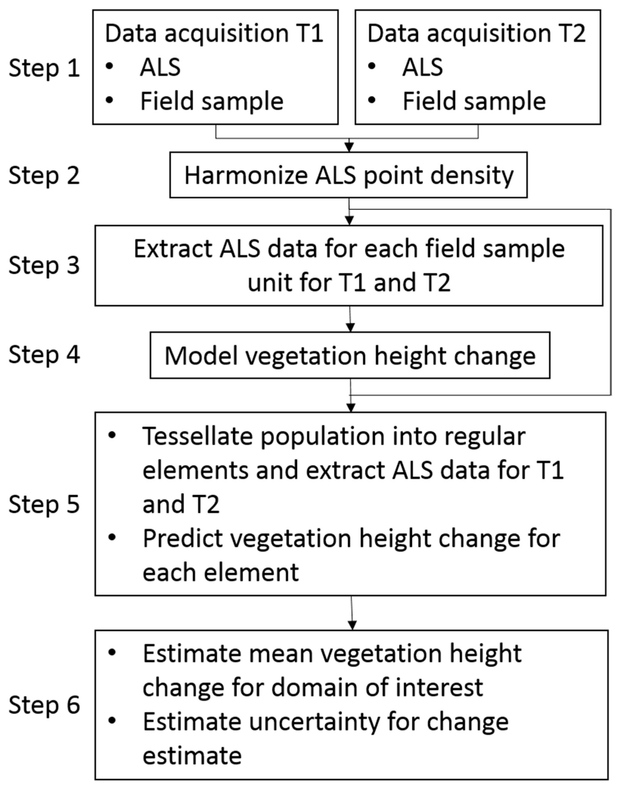
2.1. Overview of the Methodology

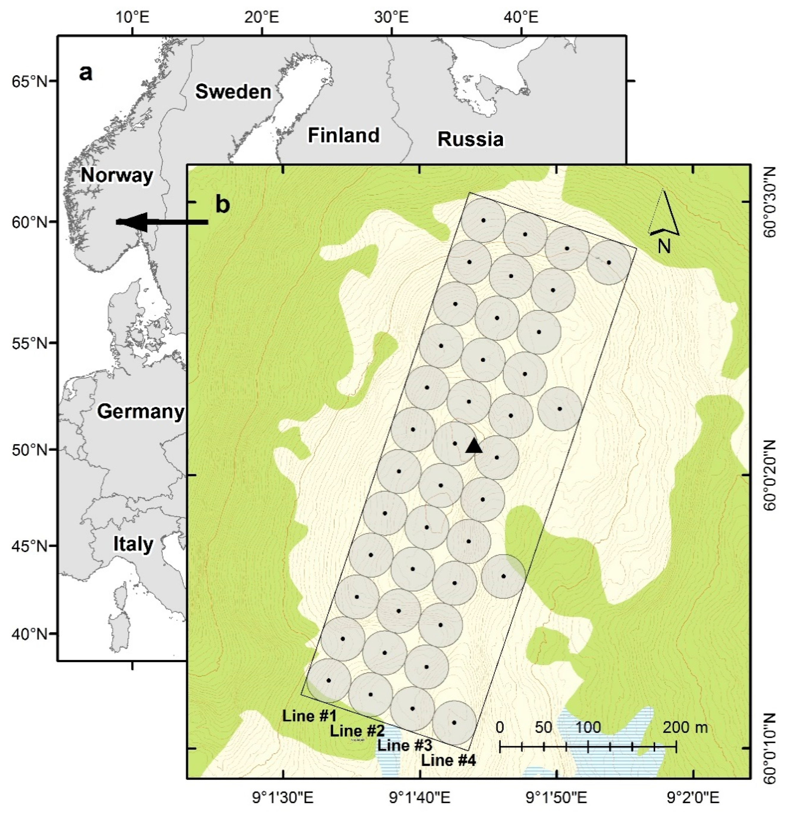
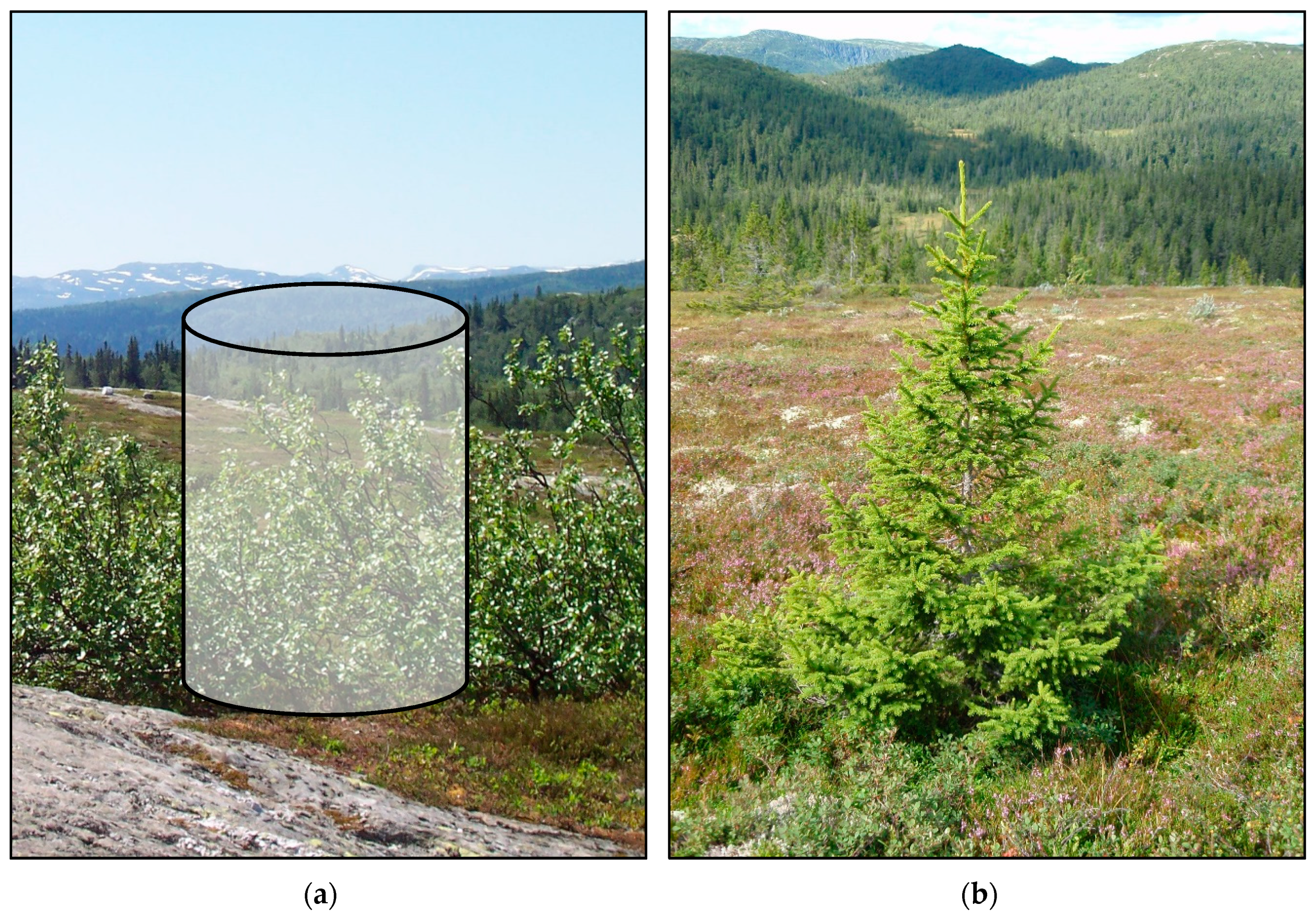
A flowchart of the entire method is displayed in Figure 1. The method entails the following six steps:

1. Wall-to-wall ALS data for the area of interest are required for the start point (T1) and the end point (T2) of the observation period. Coincident field observations of vegetation height for a sample of the same field objects must be provided at both points in time. A sample unit (field object) may be an individual tree or a vegetation cylinder or sample plot (see further details in the discussion section).

2. If the ALS pulse density differs considerably between the two datasets, methods to obtain similar densities in the two datasets may be considered.

3. ALS data are associated with the sample units, and the maximum ALS echo height at each point in time is extracted for each unit.

4. The field sample observations are used to model the change in vegetation height, with maximum vegetation height in the ALS data as the explanatory variable.

5. The area of interest is tessellated into regular population elements with the same size as the sample units, and maximum ALS height is extracted for every element for each point in time. The model from Step 4 is used to predict vegetation height change.

6. Height change is finally estimated for domains of interest following the area-based approach, for example, for individual 1.5 ha cells, as in the current demonstration of the method (see details below), larger domains, or any size domains found meaningful for a particular monitoring purpose. Estimation and inference will follow model-dependent principles, i.e., the uncertainty of the estimates will be addressed under a model-dependent inferential framework. The final product will be a spatially detailed change map and consistent inference for change.

A special application is dedicated to estimation of height changes of trees in particular, as opposed to vegetation in general. Such an application is considered useful for monitoring tree line migration. This application entails an additional modeling step (in Step 4) in which a model to predict the probability of tree is applied initially, with subsequent tree height change prediction (in Step 5) and estimation (in Step 6) for domains as detailed above. The additional model prediction step is accounted for in the uncertainty analysis (in Step 6).

In the following, we first present the data that were used in the demonstration of the method, and subsequently we detail all necessary steps described above. Finally, we present the statistical estimators (applied in Step 6) and detail an empirical analysis to quantify the magnitude of the different components of the estimator for uncertainty (Objective 2).

2.2. Study Area

The study area is located in the municipality of Rollag, southern Norway (60°0′N 9°01′E, 910–950 m above sea level) (Figure 2). The entire study was conducted within a 200 m × 600 m rectangle. The work took place in the boreal–alpine tree line, which at this location was around 900–940 m above sea level. The main tree species in the trial area were Norway spruce (Picea abies (L.) Karst.), Scots pine (Pinus sylvestris L.), and mountain birch (Betula pubescens ssp. czerepanovii). The total stem density within the study area in 2006 was estimated to be 97 trees ha⁻¹, of which only 15 trees ha⁻¹ were taller than 2 m [11].

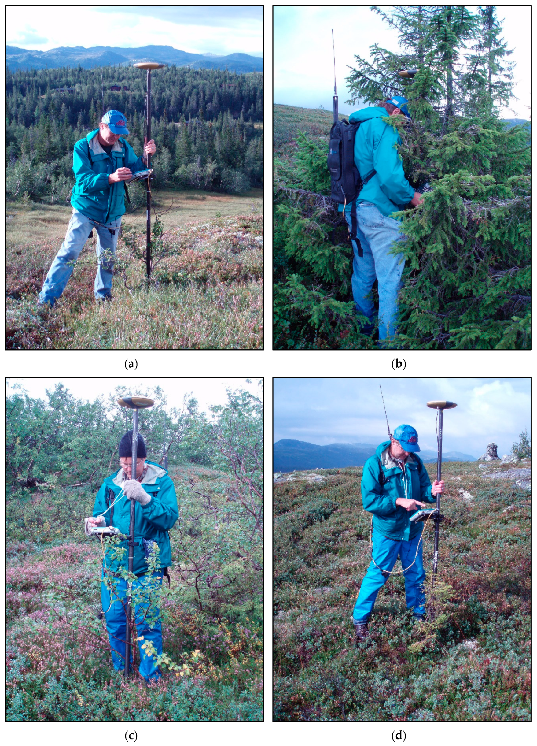
2.3. Field Measurements

The purpose of the field work was to select and georeference individual trees (sample units) that could be used as ground-reference for the analysis, and to measure physical properties that could characterize these trees. Implications of using trees as sample units are addressed in the discussion section. The field work was conducted in the period of 23–30 August 2006 and then repeated six years later, in the period 20–23 August 2012. We wanted to eliminate subjectivity in the tree selection, but at the same time cover the full range of tree heights in the area and thus provide a dataset that could support model construction.

2.3.1. Field Work in 2006

In 2006, the point-centered quarter sampling method (PCQ) [25] was used to select individual trees for the study. The tree sampling was conducted according to PCQ at 40 systematically distributed sample points within the 200 m × 600 m rectangle (Figure 2). It should be noted that due to time constraints, only four points were measured on line #4, see Figure 2.

At each point, the closest tree in each of four height classes (<1 m, 1–2 m, 2–3 m, >3 m) within each of the four quadrants around the points defined according to the cardinal directions, i.e., the NE, SE, SW, and NW quadrants, was selected. Thus, a maximum of 16 trees were selected at each point. It should be noted that the selection of trees was restricted to a maximum distance from each sample point of 25 m [26].

The stem positions of the trees were recorded with a real-time differential global positioning system (GPS) and global navigation satellite system (GLONASS), with a local reference receiver for differential correction located within the study area (Figure 2) at a national reference point of the Norwegian Mapping Authority. The expected accuracy was 3–4 cm [11]. For each tree, tree species, tree height, stem diameter at root collar, and crown diameter in two perpendicular directions (N–S and E–W) were recorded. In total, 342 trees were selected, ranging between 0.11 and 5.20 m in height. Details regarding the field work in 2006 can be found in Næsset and Nelson [11]. It is important to note that the measured trees took many different forms, including distinct and solitary trees, groups of trees—for spruce often as krumholtz, and birch appearing as solitary trees as well as in the form of tall scrubby vegetation (Figure 3). Even in the latter case (scrubby vegetation), only a single individual tree was selected and measured by strictly following the protocol outlined above.

2.3.2. Field Work in 2012

When the field work was repeated in 2012, the already defined 40 sample points were once again identified with real-time GPS + GLONASS. For each of the 40 points, the PCQ sampling was then conducted independently of the sampling in 2006, but according to the same protocol. Many of the trees selected in 2012 were the same as those measured in 2006. In addition, we identified all trees that had been measured in 2006, including those that were not selected for the 2012 PCQ sample. For the current study, we measured and analyzed all selected trees from 2006 and which still were alive in 2012. The individual tree recordings in 2012 followed the same protocol as in 2006.

2.3.3. Combining 2006 and 2012 Field Data

In the following, we let h₂₀₀₆ and h₂₀₁₂ denote field-measured tree height of an individual tree in 2006 and 2012, respectively. Among the 342 trees recorded in 2006, 316 (

Table 1. Summary of field measurements of 316 trees measured in both 2006 and 2012.

Tree Species	Characteristic	n	2006		2012
			Range	Mean	Range	Mean
Norway spruce	Tree height (m)	122	0.25–5.20	1.83	0.29–6.30	2.21
	Crown area a (m2)	122	0.034–14.522	2.314	0.061–23.562	3.070
Scots pine	Tree height (m)	31	0.11–1.01	0.41	0.28–1.59	0.70
	Crown area a (m2)	31	0.008–0.648	0.129	0.009–1.429	0.315
Mountain birch	Tree height (m)	163	0.24–4.08	1.54	0.10–3.80	1.56
	Crown area a (m2)	163	0.016–10.948	1.636	0.015–8.482	1.802
All trees	Tree height (m)	316	0.11–5.20	1.54	0.10–6.30	1.73
	Crown area a (m2)	316	0.008–14.522	1.75	0.009–23.562	2.151

^a Crown area calculated as the area of an ellipse with the perpendicular crown diameter measurements as axes.

) were still alive and were measured in 2012.

Because trees measured in the field on both occasions were required for constructing the model of height change using the ALS data (see details below), only trees that had laser recordings (laser echoes) within their crown periphery at both points in time could be used for height change modeling. Among the 316 trees, 253 trees satisfied this criterion and constituted the field dataset used for model construction.

It should be noted that even though trees that had died after 2006 were not included in the second measurement, 83 of the 316 trees that were measured twice displayed a negative height development over the observation period. Causes of negative height development could be dieback or breakage of the upper parts of tree crowns and snow pressure during winter. There was a mean increase in tree height of the 316 trees by 0.19 m (Table 1) over the course of the six years, whereas there were large differences between species (spruce: +0.38 m; pine: +0.29 m; birch: +0.02 m).

2.4. Laser Scanner Data

2.4.1. Laser Data Acquisition in 2006

ALS data were acquired on 24 July 2006 under leaf-on conditions. A fixed-wing aircraft carried the Optech ALTM 3100C laser scanning system. Average flying altitude was 700 m above ground level. Pulse repetition frequency was 100 kHz, scan frequency was 70 Hz, and maximum scan angle was ±7 degrees. Flight speed was approximately 80 ms⁻¹ and average footprint diameter was estimated to be 18 cm. Two parallel flight lines were flown over the area. However, to keep the density of recorded echoes as constant as possible across the entire study area and thus obtain a homogenous dataset with respect to laser measurement/tree interactions, echoes in the overlapping area between the two strips were discarded from either of the strips. The average echo density within the study area was 7.1 echoes m⁻².

2.4.2. Laser Data Acquisition in 2012

In 2012, the ALS data were acquired on 28 August with a Leica ALS70 laser scanner mounted on a fixed-wing aircraft. Average flying altitude was 1160 m above ground. The study area was covered by a single strip. Pulse repetition frequency was 228.4 kHz, scan frequency was 68.9 Hz, and maximum scan angle was ±8 degrees. Flight speed was approximately 70 ms⁻¹ and average footprint diameter was estimated to be 26 cm. The average echo density was 7.8 echoes m⁻².

2.4.3. Laser Data Processing

For each of the ALS datasets, the point cloud was classified into ground and non-ground echoes by the data vendors (2006: Blom Geomatics, Norway; 2012: TerraTec, Norway). The classifications were carried out with the TerraScan software [27] following the methodology described by Axelsson [28]. For the 2006 data, an iteration angle of 9.0 degrees was used and the iteration distance was 1.0 m. Corresponding parameter values for the ground classification in 2012 were 7.5 degrees and 1.9 m, respectively. The resulting digital terrain models obtained as triangulated irregular networks (TINs) were used as terrain reference surfaces, and normalized height values were computed for all “first” and “single” echoes relative to the TINs by linear interpolation. Only “first” and “single” echoes with normalized height values were used in the subsequent analysis. However, although the two laser scanners were capable of recording multiple echoes per pulse, very few pulses actually had more than a single echo due to the minimum vertical resolution between subsequent echoes for a pulse and the generally low vegetation in the area [20]. For example, for the 2012 data, only 0.17% of the pulses had multiple (>1) echoes.

2.4.4. Laser Data Thinning

In change studies based on ALS, it is important to control for differences between the ALS data acquired at different points in time in cases where ground sample data for model calibration are unavailable for each point in time.

Numerous technology-specific effects on the data may easily be confounded with the change phenomenon under study. Examples are differences in the constructed terrain elevation used as reference surface for the height normalization of the laser echoes, differences in sensor properties influencing the recorded echoes, and differences in laser data acquisition parameters such as, for example, flying altitudes, laser footprint sizes on the ground, incident angles, and pulse density.

If, however, the analysis or application in question relies on a modeled relationship between ALS data at multiple points in time and change in a vegetation property observed on the ground at coincident points in time, the modeled relationship will in fact incorporate technology-specific and acquisition-specific effects, although the different effects cannot be separated. In the current study, this was the situation; we had access to field data for individual trees that were measured at both points in time, and the model construction of change would in fact incorporate any acquisition-specific effects.

However, for the sake of generality, the following should be noted. One particular effect that actually can be circumvented with simple methods, regardless of the field data at hand, is the influence of differences in pulse density between acquisitions. The analysis of change in vegetation height in the current study was based on the maximum height value of ALS echoes within tree crown polygons (see details below). Since maximum height is an order statistic [29], it is a monotone increasing function of the number of echoes for a given target area. In the current study, the 2006 and 2012 ALS data had almost the same echo density (7.1 versus 7.8 echoes m⁻², see details above), and since there was just a single echo per pulse in the data at hand for >99% of the pulses (see above), there would be only marginal effects of differences in pulse density. However, for more pronounced differences, one might expect that greater pulse densities would result in greater maximum height values. Thinning the ALS datasets to similar densities would mitigate this effect. Numerous thinning algorithms have been proposed. For example, Magnusson et al. [30] and Gobakken and Næsset [31] tessellated the study area into regular grid cells and selected a single echo randomly within each cell, whereas Holmgren [32] discarded echoes within and between individual scans by requiring a minimum horizontal distance and a minimum difference in time of emission of the retained echoes. The latter approach aimed to mimic the pulse distributional pattern of the laser scanner. All these approaches would satisfy the requirements for change studies. Of particular interest for change studies is a method proposed by Magnussen et al. [33]. They started with the ALS dataset with the smallest pulse density, and for every echo in this dataset they searched for the nearest neighbor echo in the high-density dataset. The search was restricted by a maximum searching distance. All other echoes of the high-density dataset were discarded. Even though this thinning reduced the number of echoes in their study by about 80%, the final uncertainty of estimates of change in biomass, which was their target parameter, was only slightly reduced. In the current study, we conducted a nearest neighbor thinning, which reduced the 2012 ALS echo density from 7.8 to 7.1 echoes m⁻².

2.5. Laser Data Extraction for Sample Trees and Population Elements

Crown polygons for individual trees were constructed as ellipses around the recorded stem positions with the perpendicular crown diameter measurements (N–S, E–W) as minor and major axes. The tree crown polygons were laid atop the two ALS datasets and maximum echo height for the polygon was extracted for each point in time. These polygon-wise maximum heights were denoted as h_max2006 and h_max2012, respectively. Only the maximum ALS heights within each crown polygon were used as independent variables in the subsequent analysis in the current study (see details below), because use of, for example, deciles or moments of the ALS height distributions, which are commonly used for modeling biophysical properties of larger forest trees, would exclude a large number of trees from the dataset, because a large fraction of the small trees had only a single echo (see examples in [11]). Furthermore, the maximum ALS height of the crown polygon has previously been shown to be a strong predictor for tree height of small trees [13].

The 200 m × 600 m study area was tessellated into regular population elements of 2 m² size. This size was approximately equal to the mean crown area of the 316 trees (Table 1) in 2006 (1.75 m²) and 2012 (2.15 m²). The resulting 60,000 population elements constituted the overall population in a statistical sense (see details below). The maximum echo height was extracted for each individual element at each point in time.

2.6. Tree Height Change Model Construction

ALS-assisted estimation of change based on direct as well as indirect approaches to modeling has been demonstrated in previous studies [33,34,35,36,37]. Direct modeling entails model construction with change as the dependent variable and ALS-derived variables from both points in time or differences between corresponding variables for each point in time as independent variables. Indirect modeling entails the construction of separate models for the state variables (e.g., height or biomass) for each point in time with time-specific ALS-derived variables as independent variables in the models, or of longitudinal models with the state variable as dependent variable and with ALS-derived variables for each point in time as independent variables in the same model. Change is then estimated as the difference between predictions of the state variables. The direct method is often considered preferable because only a single set of prediction errors must be accommodated (e.g., [34,38]). In studies on design-based and model-assisted biomass change estimation supported by ALS data, Næsset et al. [35] reported marginally greater precision of estimates with the direct method, while McRoberts et al. [36] reached the opposite conclusion.

In the current study, the 253 trees mentioned above were used to model change in height. Under model-dependent inference, which was adopted in the current study due to the lack of probability samples of ground observations, the same trees would have to be used for model construction for each point in time under an indirect approach to estimation. This implies that an estimate of covariance between the mean estimates of height for the two points in time would be necessary. This would add an extra level of complexity to the uncertainty analysis. A direct approach to modeling was therefore chosen. It should be noted, though, that choice of approach to height change estimation in the boreal–alpine transition zones (direct versus indirect) may merit consideration in future studies.

A simple linear regression model with the maximum height at both points in time (h_max2006 and h_max2012, respectively) as independent variables was adopted:

$$\Delta h={\beta }_0+{\beta }_1{h}_{\max 2006}+{\beta }_2{h}_{\max 2012}+\epsilon ,$$

(1)

where $\Delta h=h_{2012}-h_{2006}$ is the field-measured change in height and ε is a normally distributed, independent error term. In an initial analysis, this model was fitted with the ordinary least-squares method. The initial analysis revealed that some observations with obvious ALS measurement errors were included in the material. Inspection of individual residuals revealed that six trees (five birch and one spruce) had higher ALS heights than the field-measured heights in the 2012 survey. They all appeared in groups of trees (see illustration in Figure 3) with taller trees in close proximity. The ALS recordings were obviously from these taller trees and not from the selected trees. Since the purpose when subsequently applying the fitted model was to predict height change based on the ALS height data for the objects that were actually measured by the laser, it would have been illogical to keep these six trees in the model, and they were therefore discarded in the final model construction. In a model based on the 247 trees, statistical tests [39,40] rejected the hypothesis of homoscedastic residuals (p < 0.01). The model was fitted using the lm function of the “stats” package with R statistical software [41]. In the presence of heteroscedasticity, heteroscedasticity-consistent covariance matrix estimators were used, as recommended by Long and Ervin [42]. The heteroscedasticity-consistent covariance matrix estimators of type HC3, presented by MacKinnon and White [43], were computed using the “sandwich” package [44] in R.

2.7. Modeling Probability of Tree

When used for prediction, the model in Equation (1) will produce height change predictions for population elements, regardless of whether the vegetation within elements consists of trees, bushes, or other ground vegetation. Some implications of using a model calibrated with tree measurement to predict change even for non-tree vegetation are further elaborated in the discussion section, and ways for improving this methodology prior to operational implementation are proposed.

For certain monitoring purposes, however, like monitoring of tree line migration, the trees, rather than vegetation in general, are of primary interest. For prediction of height change of trees in particular, a prior step is required to distinguish trees from other vegetation. As noted in the introductory section, there is hardly any information that can be derived from ALS (e.g., backscatter intensity or spatial distribution of echo heights) that can be used to effectively separate small trees from other vegetation, apart from the height information itself. We therefore developed a strategy using a prior step in which the maximum height values were used as independent variables for construction of a model for the probability of tree. However, positive height values can also represent objects other than trees, such as rocks, tussocks, and hummocks, which are common in the alpine tree line. To avoid large commission errors in tree classification based on ALS echo height, a height threshold may be introduced to separate trees from non-tree objects. In the current study area, Næsset and Nelson [11] and Næsset [21] adopted the PCQ protocol to sample and measure non-tree objects as well, and they collected 159 such objects (rocks, tussocks, and hummocks) for the 40 PCQ sample points, according to the same sampling protocol as detailed for trees (see previous sections). The maximum non-tree object height was 1.10 m, while the mean height was 0.28 m [21]. A height value of 1.10 m was therefore a reasonable threshold to distinguish between trees and non-trees. However, that also restricts the target tree sizes of a change monitoring application to relatively large trees. Clearly, this threshold must be adjusted according to local conditions. For example, in areas characterized by large boulders, such as previous ablation areas after the glacial period, the proposed methodology may have clear limitations, although other techniques, such as contextual methods, may then help to eliminate such non-tree objects from the analysis.

In the current study, we proceeded with a binomial logistic regression model with the two independent variables used in Equation (1):

$$\log \left(\frac{{\pi }_{\mathrm{TREE}}}{1-{\pi }_{\mathrm{TREE}}}\right)={\beta }_1+{\beta }_2{h}_{\max 2006}+{\beta }_3{h}_{\max 2012}+\epsilon ,$$

(2)

where ${\pi }_{\mathrm{TREE}}$ is the probability of tree defined by a height ≥1.10 m at both points in time, and h_max2006 and h_max2012 are tree-wise maximum heights from the ALS datasets from 2006 and 2012, respectively. The model was constructed using the 247 trees, among which 162 exceeded 1.10 m in height at both points in time. The model was fitted using the glm function of the “stats” package [41]. The Hosmer–Lemeshow test [45], as implemented in the “ResourceSelection” package [46], and accuracy in leave-on-out cross validation were used to assess the model fit. In the cross validation, prediction was assessed according to a classification into discrete values, i.e., if ${\pi }_{\mathrm{TREE}}$ > 0.5, it was classified as TREE. Heteroscedasticity-consistent covariance matrix estimators of type HC3 were computed using the “sandwich” package [47] in R.

Prediction of probability of tree ≥1.10 m in height was subsequently performed according to the fitted model, as follows:

$${\widehat{\pi }}_{\mathrm{TREE}}=\frac{\exp \left({\widehat{\beta }}_1+{\widehat{\beta }}_2{h}_{\max 2006}+{\widehat{\beta }}_3{h}_{\max 2012}\right)}{1+\exp \left({\widehat{\beta }}_1+{\widehat{\beta }}_2{h}_{\max 2006}+{\widehat{\beta }}_3{h}_{\max 2012}\right)}.$$

(3)

Details on how predictions by the binomial logistic model and by the height change model were combined to produce mean height change estimates for trees are provided in Section 2.9. Nevertheless, using a model to predict the probability of tree ≥1.10 m for population elements with subsequent height change prediction has the following implications for the monitoring application: the application will give greater weight to trees that had already reached a height of 1.10 m at the beginning of the observation period and which still are greater than 1.10 m in height at the end of the period. This implies that trees established during the observation period or trees that have died during the period to a lesser degree will be accounted for in the mean height change estimate. However, since the same modeling approach may be used for subsequent observation periods, trees that were established during the first period will, to a greater degree, be accounted for in the height change estimates for a later period, provided that they do not die. Likewise, trees that die after the second point in time will have a smaller impact on the height change estimates of subsequent periods. Thus, height changes will consistently tend to be attributed to target trees ≥1.10 m in height at the beginning and the end of a period, while changes in the population of target trees in the form of recruitment and mortality that break the 1.10 m height threshold will tend to be accounted for by the transition from one observation period to the next.

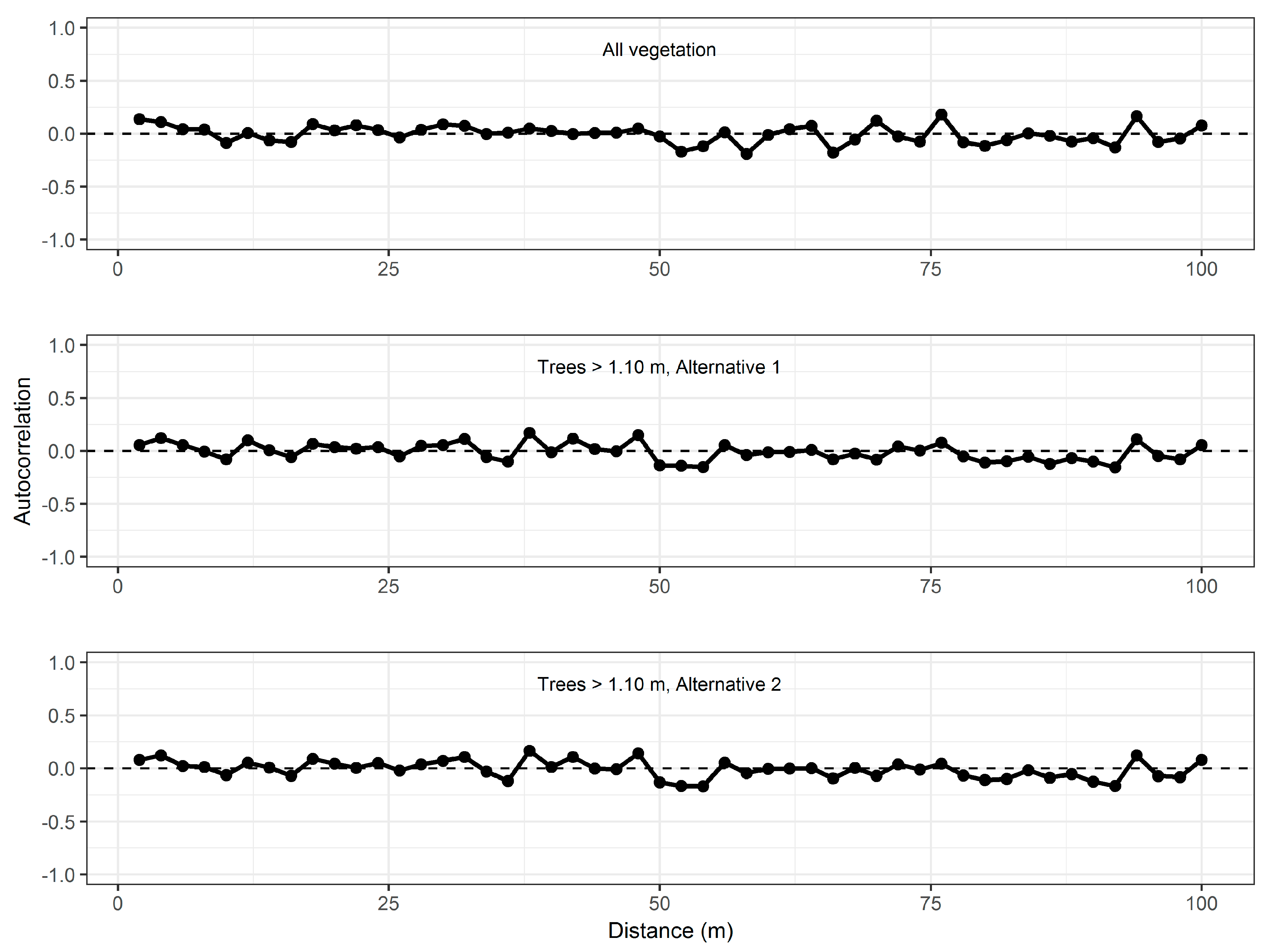
2.8. Model Parameter Independence

The analysis of the proposed application assumed that the parameter estimates of the two models Equations (1) and (2) were independent. One may suspect that estimates of parameters for the two models were correlated because both models were constructed using the same data. If parameter estimates were correlated, simultaneous parameters estimation for the two models may be considered to obtain a simultaneously estimated heteroscedasticity-consistent variance–covariance matrix.

A bootstrap resampling with 1000 repetitions was conducted, with re-fitting of the models in each repetition. The correlation between the parameter estimates was estimated and a simultaneously estimated heteroscedasticity-consistent variance–covariance matrix was obtained. This matrix was compared to the two independent matrices, estimated separately from the original sample.

The results of this evaluation showed that the independently estimated variance–covariance matrices of the two models were similar to the corresponding matrices estimated with bootstrap resampling. The four correlations among the four parameter estimates of the two models resulting from the bootstrap resampling were 0.07, 0.04, −0.07, and −0.03, respectively. Therefore, for this study, we proceeded with the initially estimated variance–covariance matrix that assumed independence. The variance–covariance matrices for the two models are displayed in

Table 2. Estimation results for linear regression model for height change fitted according to Equation (1) (n = 247).

Coefficient	Estimate	p-Value
Intercept	0.0911	<0.001
hmax2006	−0.3689	<0.001
hmax2012	0.4391	<0.001
RMSE (m)	0.293
R2	0.437
Heteroscedasticity-consistent variance–covariance matrix of parameter estimates:
Intercept	Intercept	hmax2006	hmax2012
	0.000534	−0.000197	−0.000064
hmax2006	−0.000197	0.002151	−0.001880
hmax2012	−0.000064	−0.001880	0.001927

and

Table 3. Estimation results for the logistic regression model for probability of trees ≥1.10 m in height at both points in time, fitted according to Equation (2).

Coefficient	Estimate	Wald Chi-Square	p-Value
Intercept	−2.82	43.26	<0.001
hmax2006	4.61	24.17	<0.001
hmax2012	2.13	9.56	0.002
Model fit a		4.63	0.78
Overall accuracy b (%)	87.5
Commission error for TREE b (%)	8.0
Omission error for TREE b (%)	11.1
Heteroscedasticity-consistent variance–covariance matrix of parameter estimates:
Intercept	Intercept	hmax2006	hmax2012
	0.183	−0.208	−0.155
hmax2006	−0.208	0.644	−0.093
hmax2012	−0.155	−0.093	0.522

^a Hosmer–Lemeshow statistic with 8 degrees of freedom [45]. ^b Leave-one-out cross validation with ${\pi }_{\mathrm{TREE}}$ > 0.5.

.

2.9. Model Prediction

After the models in Equations (1) and (2) were constructed, the model for height change Equation (1) was used to predict height change for all the 2 m² population elements that tessellated the study area. The result was a vegetation height change map with element-wise predictions (see Figure 6B).

Similarly, the constructed model for probability of tree ≥1.10 m in height Equation (2) was used for element-wise predictions Equation (3) for every 2 m² element across the study area. These predictions were used in two different ways in the analysis.

First, denoted “Alternative 1,” the predictions were classified as TREE or NON-TREE. If ${\widehat{\pi }}_{\mathrm{TREE}}$ > 0.5, the element was classified as TREE and assigned the value of ${\widehat{\pi }}_{\mathrm{TREE}}$ = 1. If ${\widehat{\pi }}_{\mathrm{TREE}}$ ≤ 0.5, the element was classified as NON-TREE and assigned the value of ${\widehat{\pi }}_{\mathrm{TREE}}$ = 0.

Second, denoted “Alternative 2”, the predicted probabilities of ${\widehat{\pi }}_{\mathrm{TREE}}$ for all elements were used directly without any reclassification.

2.10. Change Estimation

2.10.1. Point Estimators of Change

The general approach to estimation adopted in the proposed method is known in the literature as the area-based approach. In the current study, we did not have a probabilistic sample that would have allowed design-based inference. Model-dependent estimation and inference was therefore adopted. Model-dependent inference [48] has been applied frequently in recent years when estimating biomass, volume, and other biophysical parameters using remotely sensed data (e.g., [49,50,51,52]). An overview of the concept and a brief review of recent studies can be found in Ståhl et al. [53].

Let U be the entire population of elements (the 60,000 elements of size 2 m² that tessellate the study area) where U = {1, …, k, …, N}. Furthermore, let ${\widehat{\Delta h}}_k$ denote the predicted height change according to the model in Equation (1) for element k. Thus, the collection of spatially distributed predictions for the N elements constitutes the height change map mentioned above (Figure 6B). Mean height change across the entire study area can be estimated by

$$\overline{\widehat{\Delta h}}=\frac{{{\displaystyle \sum }}_{k\in U}{\widehat{\Delta h}}_k}{N}.$$

(4)

This estimator may be seen as a special case in which all k elements are given the same weight, namely the value 1, and therefore the sum of the weights across all k elements is equal to N. The estimator in Equation (4) may also be applied to smaller domains of U.

When, however, an estimate of mean height change for trees was sought—as opposed to change in height for vegetation in general, predictions of probability of TREE (${\widehat{\pi }}_{\mathrm{TREE}, k}$) according to the model in Equation (2) were used to weight all k elements. In the case denoted Alternative 1, the weights always took the values 1 (TREE) or 0 (NON-TREE) (see details above). In Alternative 2, the weights took the actual predicted values ${\widehat{\pi }}_{\mathrm{TREE}, k}$. The estimator can then be formulated as

$${\overline{\widehat{\Delta h}}}_{\mathrm{TREE}}=\frac{{{\displaystyle \sum }}_{k\in U}{\widehat{\Delta h}}_k {\widehat{\pi }}_{\mathrm{TREE},k}}{{{\displaystyle \sum }}_{k\in U} {\widehat{\pi }}_{\mathrm{TREE},k}}.$$

(5)

2.10.2. Estimators of Mean Square Error

Because the model-dependent estimator of the population mean cannot be assured to be unbiased, the term mean square error (MSE) rather than variance was used to characterize the uncertainty of model-dependent estimators. For large areas, model-dependent MSE estimators of the point estimators in Equations (4) and (5) will depend mainly on the uncertainty of the estimates of the model parameters (e.g., [54,55,56]). This has also been illustrated by simulation studies (e.g., [57]). For finite populations (small domains), an additional source of uncertainty must be accounted for, namely the residual error. McRoberts [58] derived a model-dependent variance estimator that accounted for residual error variance and incorporated a spatial autocorrelation structure of the residuals. Breidenbach et al. [51] demonstrated with empirical data of timber volume from small forest stands and auxiliary data from image matching of aerial photography that ignoring the residual error variance component may induce bias in the mean square error estimator. Heteroscedasticity may complicate the mean square error estimation even more [50,51,59]. In the following, we provide details on how the various mean square error components were addressed, i.e., (1) the variance due to uncertainty of the model parameters and the residual error (2) variance and (3) spatial covariance components. These three components were treated as additive to obtain the total mean square error.

Estimators Accounting for Model Parameter Uncertainty

Under the model-dependent inferential framework, the variance due to uncertainty of the model parameters can be approximated either by using a closed-form formula based on a first-order Taylor series approximation (see e.g., [55]), or by using Monte Carlo simulations in the form of, for example, parametric bootstrap. Although analytical model-dependent variance estimators that account for model parameter uncertainty have been adopted in numerous studies on forest-related properties in recent years (e.g., [49]), parametric bootstrap has several features that make it attractive in the current study. As noted by Bollandsås et al. [60], (1) it does not rely on a linear approximation, (2) it allows for estimation of the prediction errors and confidence intervals for other statistics than the mean, for example, for each individual population element, and, of particular relevance to the current study, (3) it can easily be adapted to more complex situations with several subsequent models used for predictions. The latter approach was recently demonstrated in a sample survey in interior Alaska. In the Alaska study, ALS strip samples and field surveys were adopted to estimate biomass, by which a first model with binary response (biomass/non-biomass) was used to predict the probability of biomass along the ALS strips and a second model was used to predict biomass for population elements that were predicted to contain biomass quantities greater than zero [61].

In the current study, we adopted parametric bootstrap, as in Ene et al. [61]. The technique has also been demonstrated recently in remote sensing studies by Bollandsås et al. [60] and Strîmbu et al. [62]. In the following, it is assumed that the model parameter estimates of the predictive models ($\beta$ in the models in Equations (1) and (2) are independent (see Section 2.8) and follow asymptotically multivariate normal distributions, i.e.,

$$\widehat{\mathsf{\beta }}~\mathrm{N}\left(\mathrm{E}\left[\mathsf{\beta }\right],{\Sigma }_{\widehat{\mathsf{\beta }}}\right),$$

(6)

where the expected value of the vector of $\widehat{\mathsf{\beta }}$ estimates is $\mathrm{E}\left[\mathsf{\beta }\right]$ and ${\Sigma }_{\widehat{\mathsf{\beta }}}$ is the heteroscedasticity-consistent estimates of the variance–covariance matrix of $\widehat{\mathsf{\beta }}$.

First, we wanted to establish a bootstrap procedure for a case in which only one model was involved, i.e., estimation of mean change in vegetation height following the model in Equation (1) and the estimator in Equation (4). By sampling from the multivariate distribution in Equation (6), a large parametric bootstrap sample of random vectors ${\mathsf{\beta }}_{\mathrm{PB}}~\mathrm{N}\left(\widehat{\mathsf{\beta }},{\Sigma }_{\widehat{\mathsf{\beta }}}\right)$ was generated. The sample was denoted S_PB, where S_PB = {1, …, l, …, M}. This sample can be used to produce new predictions of $\Delta h$, according to Equation (1). Predictions of $\Delta h$ were produced for all M random vectors ${\mathsf{\beta }}_{\mathrm{PB}}$ and for all N population elements. Thus, we obtained unique predictions ${\widehat{\Delta h}}_{\mathrm{PB},k,l}$ for $k\in U$ and $l\in S_{\mathrm{PB}}$. A parametric bootstrap variance estimator for the point estimator in Equation (4) is

$$\mathrm{var}{\left(\overline{\widehat{\Delta h}}\right)}_{\mathrm{par}}=\frac{1}{M-1}{{\displaystyle \sum }}_{l\in S_{\mathrm{PB}}}{\left({\widehat{\Delta h}}_{\mathrm{PB},l}-{\widehat{\Delta h}}_{\mathrm{PB}}\right)}^2,$$

(7)

where

$${\widehat{\Delta h}}_{\mathrm{PB},l}=\frac{1}{N}{{\displaystyle \sum }}_{k\in U}{\widehat{\Delta h}}_{\mathrm{PB},k,l}$$

(8)

and

$${\widehat{\Delta h}}_{\mathrm{PB}}=\frac{1}{M}{{\displaystyle \sum }}_{l\in S_{\mathrm{PB}}}{\widehat{\Delta h}}_{\mathrm{PB},l}.$$

(9)

When two subsequent prediction models were involved in the estimation to obtain height change estimates of trees only, estimation of the uncertainty of the height change predictions became more complicated. In addition to the bootstrap sample of random vectors ${\mathsf{\beta }}_{\mathrm{PB}}$ in Equation (6), a parametric bootstrap sample of random vectors ${{\mathsf{\beta }}^{\prime }}_{\mathrm{PB}}~\mathrm{N}\left({\widehat{\mathsf{\beta }}}^{\prime },{\Sigma }_{{\widehat{\mathsf{\beta }}}^{\prime }}\right)$, denoted ${S^{\prime }}_{\mathrm{PB}}$, was generated for the model in Equation (2) as well. Here, ${S^{\prime }}_{\mathrm{PB}}$ = {1, …, p, …, Q}. For each vector p among the Q vectors, a prediction of ${\widehat{\pi }}_{\mathrm{TREE}}$ was produced for all Q random vectors ${{\mathsf{\beta }}^{\prime }}_{\mathrm{PB}}$ and for all N population elements. This resulted in unique predictions ${\widehat{\pi }}_{\mathrm{TREE}, \mathrm{PB},k,p}$ for $k\in U$ and $p\in {S^{\prime }}_{\mathrm{PB}}$.

A parametric bootstrap variance estimator for the point estimator in Equation (5) was then obtained by combining all Q simulated realizations of ${\widehat{\pi }}_{\mathrm{TREE}}$ with the M simulated realizations of $\widehat{\Delta h}$. The variance estimator can be formulated as

$$\mathrm{var}{\left({\overline{\widehat{\Delta h}}}_{\mathrm{TREE}}\right)}_{\mathrm{par}}=\frac{1}{QM-1}{{\displaystyle \sum }}_{p\in {S^{\prime }}_{\mathrm{PB}}}{{\displaystyle \sum }}_{l\in S_{\mathrm{PB}}}{\left({\widehat{\Delta h}}_{\mathrm{TREE},\mathrm{PB},l,p}-{\widehat{\Delta h}}_{\mathrm{TREE},\mathrm{PB}}\right)}^2,$$

(10)

where

$${\widehat{\Delta h}}_{\mathrm{TREE},\mathrm{PB},l,p}=\frac{{{\displaystyle \sum }}_{k\in U}{\widehat{\Delta h}}_{\mathrm{PB},k,l}{\widehat{\pi }}_{\mathrm{TREE},\mathrm{PB},k,p}}{{{\displaystyle \sum }}_{k\in U}{\widehat{\pi }}_{\mathrm{TREE},\mathrm{PB},k,p}}$$

(11)

and

$${\widehat{\Delta h}}_{\mathrm{TREE},\mathrm{PB}}=\frac{1}{QM}{{\displaystyle \sum }}_{p\in {S^{\prime }}_{\mathrm{PB}}}{{\displaystyle \sum }}_{l\in S_{\mathrm{PB}}}{\widehat{\Delta h}}_{\mathrm{TREE},\mathrm{PB},l,p}.$$

(12)

As for the point estimator in Equation (5), the variance was estimated for the two approaches, Alternative 1 and Alternative 2. In the case denoted Alternative 1, the weights (${\widehat{\pi }}_{\mathrm{TREE},\mathrm{PB},k,p})$ always took the values 1 (TREE) or 0 (NON-TREE), according to the rules outlined above. In Alternative 2, the weights took the actual predicted values.

Estimators Accounting for Residual Variance

Analytical estimators of residual variance under heteroscedasticity have been adopted in previous analysis of important parameters encountered in forest surveys, such as forest area, volume, and biomass (e.g., [50,51,58]). In the current study, every geographical domain subject to estimation and analysis had sample units (ground observations of height change) that could be used to provide estimates of residual variance. Thus, for a particular domain with a sample S with n sample units, S = {1, …, k, …, n}, the residual variance for the point estimator for mean vegetation height change Equation (4) can be formulated as

$$\mathrm{var}{\left(\overline{\widehat{\Delta h}}\right)}_{\mathrm{res}}=\frac{1}{Nn}{{\displaystyle \sum }}_{k\in S}{\left(\Delta h_k-{\widehat{\Delta h}}_k\right)}^2.$$

(13)

For the point estimator of mean height change of trees ≥1.10 m Equation (5), we obtain

$$\mathrm{var}{\left({\overline{\widehat{\Delta h}}}_{\mathrm{TREE}}\right)}_{\mathrm{res}}=\frac{1}{Nn}{{\displaystyle \sum }}_{k\in S}{\left(\Delta h_k{I}_k-{\widehat{\Delta h}}_k{\widehat{\pi }}_{\mathrm{TREE},k}\right)}^2,$$

(14)

where I_k is an indicator of TREE (I_k = 1) or NON-TREE (I_k = 0).

As for the variance estimator in Equations (10)–(12), the residual variance was estimated for the two approaches, Alternative 1 and Alternative 2.

Estimators Accounting for Residual Covariance

Residual covariance of substantial magnitude, as compared to the other sources of uncertainty when estimating forest resource parameters for small areas, has been encountered for shorter distances in several studies (e.g., [50,51]), while at greater distances—and consequently for larger areas—the residual covariance is often assumed or found to be negligible in magnitude [50,55]. Analytical ways of addressing the residual covariance have been demonstrated by, for example, Breidenbach et al. [51]. An essential part of the analysis of the residual covariance is the determination of the spatial autocorrelation of the residuals. Spatial correlation, ρ, is often estimated via a correlogram using the model prediction residuals when fitting the correlogram. Assuming that a correlogram has been fitted and that ρ can then be predicted to obtain predicted values of the correlation for all combinations of the N population elements in U, the residual covariance for the point estimator of mean vegetation height change Equation (4) for a particular domain for which we had actual observations of the residuals, can be estimated by

$$\mathrm{cov}{\left(\overline{\widehat{\Delta h}}\right)}_{\mathrm{res}}=\frac{1}{n{N}^2}{{\displaystyle \sum }}_{k\in S}{\left(\Delta h_k-{\widehat{\Delta h}}_k\right)}^2{{\displaystyle \sum }}_{k\in U}{{\displaystyle \sum }}_{l\in U}{\widehat{\rho }}_{kl}, k\ne l ,$$

(15)

where ${\widehat{\rho }}_{kl}$ is the predicted value of the residual correlation between elements k and l in U and the correlogram was fitted using the residuals $\Delta h_k-{\widehat{\Delta h}}_k$ and $\Delta h_l-{\widehat{\Delta h}}_l$.

Similarly, for the point estimator of mean height change of trees ≥1.10 m Equation (5), the corresponding residual covariance can be estimated according to

$$\mathrm{cov}{\left({\overline{\widehat{\Delta h}}}_{\mathrm{TREE}}\right)}_{\mathrm{res}}=\frac{1}{n{N}^2}{{\displaystyle \sum }}_{k\in S}{\left(\Delta h_k{I}_k-{\widehat{\Delta h}}_k{\widehat{\pi }}_{\mathrm{TREE},k}\right)}^2{{\displaystyle \sum }}_{k\in U}{{\displaystyle \sum }}_{l\in U}{\widehat{\rho }}_{kl},k\ne l,$$

(16)

where the correlogram was fitted using the residuals $\Delta h_k{I}_k-{\widehat{\Delta h}}_k{\widehat{\pi }}_{\mathrm{TREE},k}$ and $\Delta h_l{I}_l-{\widehat{\Delta h}}_l{\widehat{\pi }}_{\mathrm{TREE},l}$.

2.10.3. Assessment of Bias Properties of the Point Estimators

Assessment of the bias properties of the estimator for mean height change for all vegetation and the two estimators for mean height change for trees ≥1.10 m (Alternatives 1 and 2) can only be performed by exhaustive simulations in which the entire population is known. In practice, that can only be achieved by using an artificial population. Such a task was outside of the scope of the current study.

However, (1) when the model(s) exhibits no systematic lack of fit to the sample data and (2) the moments of the independent variables in the sample correspond well to the moments of the population values, estimators of the mean are generally considered unbiased. We assessed the fit of the models and calculated the two first moments.

Furthermore, because we adopted in the most complex case of estimating height change for trees ≥1.10 m a sequence of two subsequent model predictions, we also assessed the resulting residuals of this two-step prediction procedure to identify any potential lack of fit in the two-step case. This was done by estimating and observing the mean error for the sample according to

$$\mathrm{ME}=\frac{{{\displaystyle \sum }}_{k\in S}{\widehat{\Delta h}}_k{\widehat{\pi }}_{\mathrm{TREE},k}}{{{\displaystyle \sum }}_{k\in S} {\widehat{\pi }}_{\mathrm{TREE},k}}-\frac{{{\displaystyle \sum }}_{k\in S}\Delta h_k{I}_k}{{{\displaystyle \sum }}_{k\in S}{I}_k},$$

(17)

where, as before, the weights (${\widehat{\pi }}_{\mathrm{TREE},k})$ always took the values 1 (TREE) or 0 (NON-TREE) for Alternative 1 according to the rules outlined above, while in Alternative 2, the weights took the actual predicted values.

2.11. Analysis

The first step of the analysis was to construct the regression model for change in vegetation height based on the 247 trees that were measured twice (Section 2.6). Subsequently, the logistic regression model for probability of tree ≥1.10 m in height was fitted with the same trees (Section 2.7).

Once the regression models were constructed, we proceeded with the estimation. First, we estimated mean change in vegetation height across the entire study area, according to Equation (4), by using model predictions from the height change model Equation (1). We then estimated mean change in height for trees ≥1.10 m. This was done according to the estimator in Equation (5) by using model predictions of probability of tree Equation (3) and model predictions of height change Equation (1).

Two demonstration cases of special interest were identified. First (Case A), we tessellated the study area into 1.5 ha cells that may serve as the primary monitoring units in, for example, a tree line monitoring program. This size was chosen purely for demonstration purposes, and this size can be changed to any size found meaningful for a particular monitoring purpose. Nevertheless, a size of 1.5 ha would allow a tessellation of the current study area into eight individual cells, which is useful to demonstrate to what extent cells of the chosen size would capture statistically significant differences in height growth. Further, as residual covariance may be an issue in model-dependent inference for small areas, we took the opportunity to evaluate the magnitude of the different components of the MSE estimate for this particular size, as this may inform whether 1.5 ha or even smaller areas may be meaningful sizes in future designs of monitoring applications.

Second (Case B), despite the very limited geographical extent of the study area (200 m × 600 m), it displayed variation in wind exposure, temperature, soil depth, and moisture due to its location on and along a small ridge with variations in aspect. As discussed by Kambo and Danby [63], these are all factors influencing seedling establishment, growth, and mortality in tree line environments, and aspect-related differences have been established in the literature in multiple forest, tree line, and tundra sites [63]. Thus, we divided the area into four sub-regions (see Figure 6A) according to aspect, slope, elevation, and soil depth (occurrence of bedrock outcrops). This was done on the basis of aerial photography, the digital terrain model, and the structure of the vegetation as it appeared in the ALS data. These sub-regions may reflect biologically meaningful differences in vegetation and tree productivity, and this Case B was included to demonstrate how the proposed method could be used for ecologically oriented analysis. It should be noted, though, that the focus was on technical aspects of the estimation process and not on a biological interpretation of the results. Estimates of change in vegetation height and tree height were produced for these four sub-regions as well.

The final step of the analysis was to estimate the various MSE components for the entire study area and for each geographical domain (eight 1.5 ha cells and four sub-regions) subject to analysis. This analysis started with the construction of separate correlograms for the residuals for each domain of interest. Correlations based on the observed residuals were graphed and then visually inspected. For natural phenomena, in general, it is common to observe greater correlations at shorter distances and then declining correlations with increasing distances. Such spatial structures can be modeled, for example, by some exponential model form. In the current dataset, no such spatial structure could be observed (see examples in Figure 4). Simple linear regression models of the form

$$\rho ={\beta }_0+{\beta }_{1}D+\epsilon$$

(18)

appeared to be suitable, where D is the distance between pairs of residuals. In total, 39 correlogram models were constructed according to Equation (18), i.e., separate models for each domain subject to estimation, and for change in vegetation height for all vegetation and for trees ≥1.10 m in height. Examples of these models are graphed in Figure 4.

The results of the model construction revealed p-values of ${\widehat{\beta }}_0$ ranging from 0.08 to 0.99 for 37 of the 39 models. Similarly, the p-values of ${\widehat{\beta }}_1$ were in the range of 0.09 to 0.96 for the 37 models. When ${\widehat{\beta }}_1$ is not statistically significantly different from zero, the residual correlation can be considered constant across different spatial ranges. Furthermore, when ${\widehat{\beta }}_1$ is not statistically significantly different from zero, the spatially constant correlation is actually zero as well. We therefore concluded that the residual covariance components of the estimates of MSE ($\widehat{\mathrm{MSE}}$) would be zero and could be ignored in these 37 cases. In the two remaining cases, namely the models for Alternatives 1 and 2 in Cell #2 (see Figure 6A), ${\widehat{\beta }}_0$ and ${\widehat{\beta }}_1$ were positive and negative, respectively, such that at the average distance of the (N – 1)N pairs of the covariance estimator (65.8 m), the two autocorrelation models would result in predicted values of ${\widehat{\rho }}_{kl}$ close to zero. Even in these two cases, the residual covariance could therefore be ignored cf. Equation (16).

In the characterization of the uncertainty of the various point estimates of height change, we therefore proceeded with estimating MSE by adding the two remaining variance components, accounting for model parameter uncertainty Equations (7) and (10) and residual variance Equations (13) and (14). Subsequently, we calculated the standard error of the mean estimate (SE; square root of $\widehat{\mathrm{MSE}}$) and a 95% confidence interval of the mean estimate. The proportions of $\widehat{\mathrm{MSE}}$ that were attributed to the residual variance were also calculated.

In the bootstrap variance estimation used to characterize the model parameter uncertainty, the bootstrap was repeated until the mean variance over replications stabilized. Stabilization was judged by visual inspection of graphical plots of the mean variance. For some of the estimates, stable variances were obtained with fewer than 1000 simulated realizations, while for other estimates, 2000 realizations were needed to reach stable estimates. Thus, 2000 realizations were used in all simulations reported in this study.

Finally, we estimated the mean error of the mean height change estimates of the trees ≥1.10 m for Alternatives 1 and 2 for the entire study area, and for the smaller domains using the trees observed in the field. The mean error was estimated according to Equation (17).

3. Results and Discussion

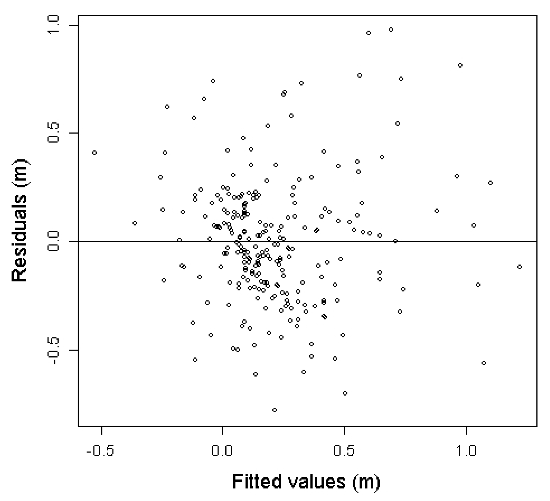
3.1. Model Construction

Results for the models for height change based on the 247 trees are displayed in Table 2, which also includes the estimated heteroscedasticity-consistent variance–covariance matrix for the parameter estimates that was needed for the parametric bootstrap variance estimation.

All parameter estimates were highly significant (p < 0.001) and the model displayed an adequate fit to the data with R² = 0.437 and RMSE = 0.293 m. The signs of all parameter estimates were also logical, with a negative sign for the parameter estimate for the ALS variable of height from the first point in time (h_max2006) and positive for the last point in time (h_max2012). The residual graph (Figure 5) did not indicate any model misspecification.

To the very best of our knowledge, there has been only one previous study conducted under similar conditions that may serve as a reference for our analysis. Hauglin et al. [13] constructed models for tree height change for small pioneer trees in a 1500 km long ALS transect encompassing numerous boreal–alpine transition zones from 58° N to 69° N in Norway. Their analysis included 262 trees from 35 locations along the transect, which were observed over a time period of 4 years. On average, the trees were 0.25–0.30 m taller than in the current study, and a similar model form was adopted. They reported an R² = 0.36, well in line with current findings, and RMSE = 0.16 m, which was smaller than in the current study.

The logistic regression model for the probability of trees ≥1.10 m in height at both points in time showed adequate fit to the data (Table 3). This was confirmed by the Hosmer–Lemeshow statistic (p = 0.780). Greater p-values would suggest correctly specified models, while p-values less than, for example, 0.05 would suggest a model with inadequate fit. Cross validation of the model showed an overall accuracy of 87.5%. All parameter estimates were statistically significantly different from 0 (p ≤ 0.002).

3.2. Overall Change Estimates

The estimated mean change in vegetation height across the entire study area was 0.16 m (SE = 0.020 m) over the full observation period, while the estimated mean change in height for trees ≥1.10 m in height was 0.29 m (SE = 0.027 m) when the predicted probabilities of tree were reclassified to 0/1 (Alternative 1) and 0.24 m (SE = 0.024) when the actual predicted probabilities of tree (Alternative 2) were used (

Table 4. Estimates of mean change in vegetation height ($\widehat{\overline{\Delta h}}$; Equation (4) and in height of trees ≥1.10 m (${\widehat{\overline{\Delta h}}}_{\mathrm{TREE}}$; Equation (5) for various domains of the study area, and corresponding standard error estimates ^a (SE) and 95% confidence intervals (CI).

Domain	All Vegetation (m)					Trees ≥1.10 m (m)
						Alternative 1 b					Alternative 2 c
	$$\widehat{\overline{\mathbf{\Delta }\mathit{h}}}$$	SE	CI			$${\widehat{\overline{\mathbf{\Delta }\mathit{h}}}}_{\mathbf{TREE}}$$	SE	CI			$${\widehat{\overline{\mathbf{\Delta }\mathit{h}}}}_{\mathbf{TREE}}$$	SE	CI
Study area	0.16	0.020	0.12	-	0.20	0.29	0.027	0.24	-	0.34	0.24	0.024	0.19	-	0.28
Case A:
Cell 1	0.14	0.022	0.10	-	0.18	0.24	0.023	0.19	-	0.28	0.18	0.021	0.14	-	0.22
Cell 2	0.14	0.022	0.10	-	0.18	0.21	0.021	0.16	-	0.25	0.16	0.020	0.12	-	0.20
Cell 3	0.18	0.019	0.14	-	0.22	0.30	0.030	0.24	-	0.36	0.26	0.026	0.21	-	0.31
Cell 4	0.16	0.019	0.12	-	0.20	0.23	0.024	0.18	-	0.28	0.21	0.022	0.16	-	0.25
Cell 5	0.15	0.021	0.11	-	0.19	0.28	0.024	0.23	-	0.32	0.22	0.023	0.18	-	0.27
Cell 6	0.14	0.022	0.10	-	0.18	0.28	0.024	0.23	-	0.32	0.20	0.023	0.16	-	0.25
Cell 7	0.13	0.023	0.09	-	0.17	0.21	0.020	0.17	-	0.25	0.15	0.021	0.11	-	0.19
Cell 8	0.22	0.019	0.18	-	0.26	0.37	0.035	0.31	-	0.44	0.34	0.032	0.28	-	0.40
Case B:
Sub-region I	0.14	0.022	0.10	-	0.19	0.29	0.026	0.24	-	0.34	0.21	0.024	0.16	-	0.26
Sub-region II	0.14	0.022	0.10	-	0.18	0.23	0.022	0.18	-	0.27	0.18	0.020	0.14	-	0.22
Sub-region III	0.17	0.020	0.13	-	0.21	0.28	0.026	0.23	-	0.33	0.23	0.023	0.19	-	0.28
Sub-region IV	0.19	0.019	0.15	-	0.23	0.34	0.031	0.28	-	0.40	0.30	0.028	0.24	-	0.35

^a Standard error based on the sum of the variance due to parameter uncertainty and residual variance. ^b Probability of tree ≥1.10 m in height reclassified to 0 (NON-TREE) and 1 (TREE).^c Probability of tree ≥1.10 m in height according to actual predicted probabilities (${\widehat{\pi }}_{\mathrm{TREE}}$).

). Thus, the annual mean change was 2.6 cm for all vegetation and 4.9 and 4.0 cm for trees ≥1.10 m in height, depending on how the predicted probabilities were treated. The 95% confidence intervals indicated that the estimated height changes over the whole period were significantly greater than zero for all vegetation, as well as for trees.

These results indicate that ALS is sensitive to height changes of vegetation and small trees, even for very short observation periods—in this case, only 6 years. Interestingly, the estimates indicate a net growth in height for the study area as a whole. However, such results can hardly say anything about the causes of change, but for this particular area, it is likely that changing land use over the past decades can at least partly explain the changes, as there were numerous summer farms in the area that dated back centuries and that were abandoned during the mid-1900s.

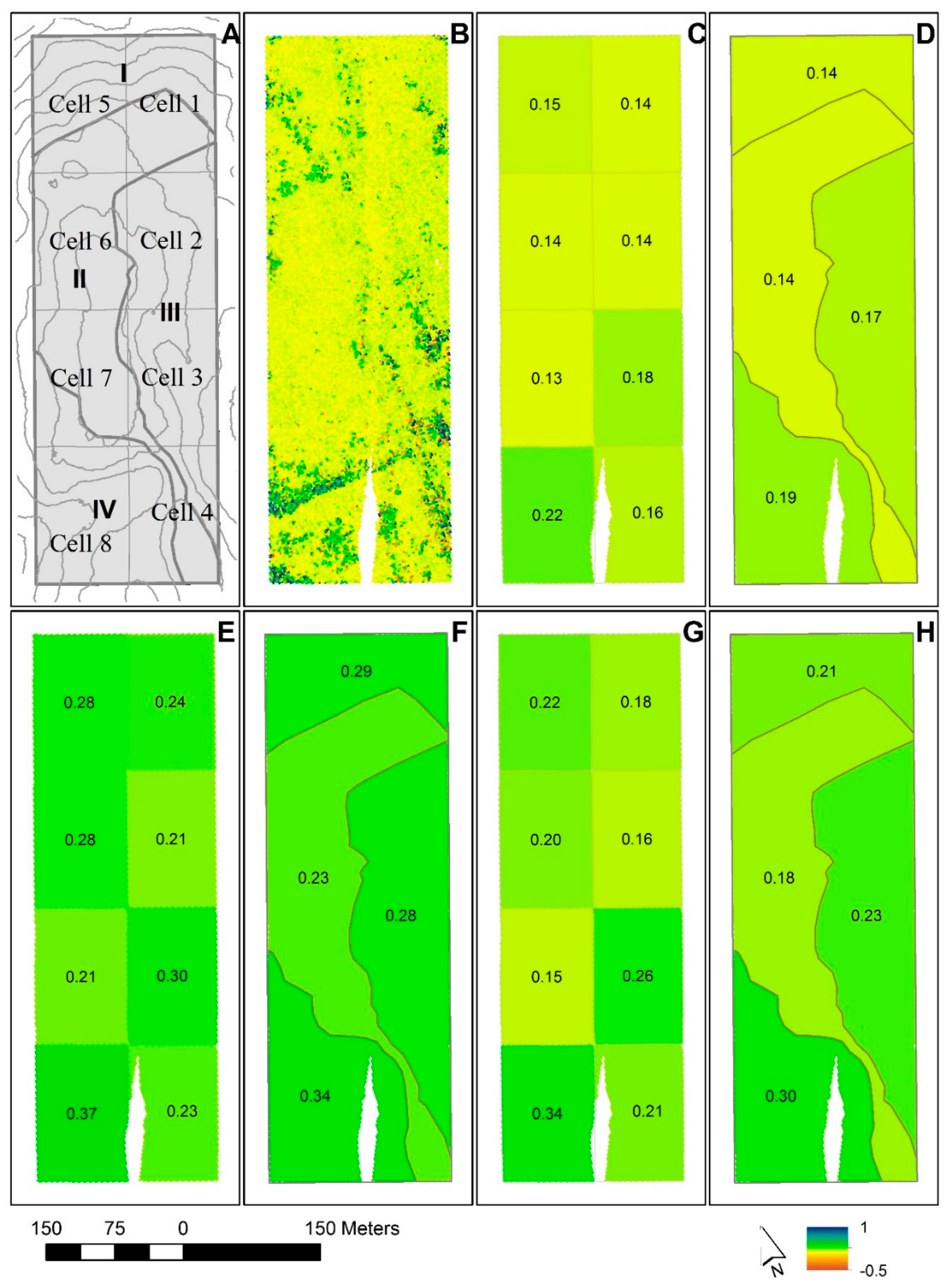
3.3. Change Estimates for Domains

The mean change estimates for the 1.5 ha cells (Case A) ranged from 0.13 m to 0.22 m for vegetation in general (Table 4, Figure 6C), and from 0.21 m to 0.37 m for the trees under Alternative 1 (Figure 6E) and from 0.15 m to 0.34 m for Alternative 2 (Figure 6G). The 95% confidence intervals indicated that all change estimates were significantly greater than zero.

In this particular study area, the confidence intervals indicated that the height changes for all vegetation differed significantly among cells. The change estimate for Cell #8 of 0.22 m was significantly greater than estimates for Cells #1, #2, and #7 of 0.14 m, 0.14 m, and 0.13 m, respectively (see Figure 6C). This illustrates that for monitoring units of, for example, 1.5 ha in size, it should be possible to identify gradients in vegetation change, at least if the observation period is of a minimum length of around 10 years, and particularly so with longer or steeper elevation gradients than in the current study area. It should be noted, though, that when multiple statistical comparisons (tests) are performed simultaneously, one may wish to alter the level of significance to control the total Type I error (Bonferroni approach [64]). Especially for studies of vegetation changes over larger areas covering many monitoring units, this may be an important consideration.

For the trees ≥1.10 m in height under Alternative 2, the height change estimate for Cell #8 of 0.34 m was clearly significantly greater than estimates for Cells #1–2 and #4–7, which ranged from 0.15 m to 0.22 m. Likewise, the change estimate for Cell #3 (0.26 cm) was significantly greater than estimates for Cells #2 (0.16 m) and #7 (0.15 m). Similar results were found for Alternative 1. This suggests that significant gradients even in tree height change may be identified. The proposed estimators may therefore support efforts to monitor tree line migration over time.

The subjectively defined sub-regions (Case B) based on aspect, slope, elevation, and soil depth (occurrence of bedrock outcrops) showed slight differences in estimated mean height growth, at least among some of the sub-regions. For all vegetation (Figure 6D), the mean height change estimate ranged from 0.14 m for sub-region II, which was located on top of the ridge with shallow soils and frequent occurrences of bedrock outcrops, to 0.19 m for sub-region IV, with a flat to southwesterly aspect, deeper soils, and more protected location against wind than on the top of the ridge. The 95% confidence intervals for the estimates for these two extreme sub-regions did not confirm that the differences were statistically significant, however (Table 4). For the trees ≥1.10 m in height, estimated mean height changes for sub-regions II and IV were statistically significantly different. The estimated changes in height for these two regions were 0.23 m and 0.34 m under Alternative 1 (Figure 6F), respectively, and 0.18 m and 0.30 m under Alternative 2 (Figure 6H). Given the characteristics of the sub-regions, these results are all logical, and the analysis demonstrates that the proposed estimators can even be used to find ecologically meaningful changes in the vegetation and tree heights, and thus be used to shed light on ecological processes in the boreal–alpine ecotone.

3.4. Model-Dependent Inference for Domains

One of the objectives of this study was to provide estimators for uncertainty of the estimated change in height of trees and vegetation in general and by that provide a basis for statistical inference. When we estimated the $\widehat{\mathrm{MSE}}$ components for the different sources of uncertainty, we noted that in the current dataset the residual covariance could be ignored because the spatial autocorrelation of the residuals was zero or close to zero – even for the smaller 1.5 ha cells (see Section 2.11). The constant and negligible residual spatial correlation across different lag distances suggests that residual covariance may be ignored for inference regarding height change even for domains smaller than 1.5 ha.

Even the residual variance was of marginal magnitude. The residual variance accounted for 0.2–0.4% of $\widehat{\mathrm{MSE}}$ for the entire study area (

Table 5. Contribution of the residual variance component to overall mean square error of estimates of change in vegetation height ($\mathrm{var}{\left(\widehat{\overline{\Delta h}}\right)}_{\mathrm{res}}$) and change in height of trees ≥1.10 m in height ($\mathrm{var}{\left({\widehat{\overline{\Delta h}}}_{\mathrm{TREE}}\right)}_{\mathrm{res}}$) and mean error (ME) estimated according to e.g. (17).

Domain	n	All Vegetation	Trees ≥1.10 m
			Alternative 1 a		Alternative 2 b
		$$\begin{gathered} \mathbf{var}{\left(\widehat{\overline{\mathbf{\Delta }\mathit{h}}}\right)}_{\mathbf{res}} \\ (\%) \end{gathered}$$	ME (m)	$$\begin{gathered} \mathbf{var}{\left({\widehat{\overline{\mathbf{\Delta }\mathit{h}}}}_{\mathbf{TREE}}\right)}_{\mathbf{res}} \\ (\%) \end{gathered}$$	ME (m)	$$\begin{gathered} \mathbf{var}{\left({\widehat{\overline{\mathbf{\Delta }\mathit{h}}}}_{\mathbf{TREE}}\right)}_{\mathbf{res}} \\ (\%) \end{gathered}$$
Study area	247	0.4	0.028	0.2	0.021	0.2
Case A:
Cell 1	25	1.6	0.104	0.5	0.052	0.5
Cell 2	23	1.2	0.019	1.0	0.013	0.9
Cell 3	26	2.9	−0.047	1.1	−0.046	1.5
Cell 4	35	4.1	0.008	2.4	0.004	2.9
Cell 5	43	2.4	0.061	1.8	0.056	1.8
Cell 6	25	1.6	0.081	1.0	0.068	1.0
Cell 7	21	2.1	0.108	1.5	0.084	1.2
Cell 8	49	5.1	−0.017	1.3	−0.008	1.6
Case B:
Sub-region I	42	2.0	0.084	1.3	0.063	1.4
Sub-region II	66	0.6	0.088	0.3	0.073	0.4
Sub-region III	51	1.0	−0.034	0.5	−0.036	0.6
Sub-region IV	88	2.7	0.005	0.9	0.006	1.1

^a Probability of tree ≥1.10 m in height reclassified to 0 (NON-TREE) and 1 (TREE). ^b Probability of tree ≥1.10 m in height according to actual predicted probabilities (${\widehat{\pi }}_{\mathrm{TREE}}$).

). For the change estimates for trees (Alternatives 1 and 2) for the various domains, the residual variance accounted for only 0.3–2.9% of $\widehat{\mathrm{MSE}}$. For all vegetation, the corresponding contribution to $\widehat{\mathrm{MSE}}$ was 0.6–2.9% for all domains, except for two of the 1.5 ha cells, for which the residual variance accounted for 4.1% (Cell #4) and 5.1% (Cell # 8) of $\widehat{\mathrm{MSE}}$. The overall assessment is therefore that in applications like those analyzed in the current study, the variance due to uncertainty of the model parameters may account for around 95% or more of the total $\widehat{\mathrm{MSE}}$ of the mean estimate, even when the domains are small. It should be noted that the area under study was small, and that caution should be exercised in generalizing from these findings. Nevertheless, it was observed that there was no clear evidence of differences in residual variance between the sub-regions with smallest vegetation and smallest change (sub-regions I–II) and tallest vegetation and largest change (sub-regions III–IV), cf. Table 4 and Table 5. Despite the small extent of the study area, this suggests that the relative magnitude of the residual variance may not be sensitive to the properties of the vegetation in the ecotone.

3.5. Bias Properties of the Point Estimators

The two fitted models did not exhibit any systematic lack of fit to the sample data (see details in Section 3.1). The second moments of the distributions of the independent variables (h_max2006 and h_max2012) were of similar magnitude in the sample data and in the population. Further, the analysis of the mean residual errors for the actual sample of field-measured trees revealed that only minor mean errors were present even for the complex cases of two subsequent model predictions (Alternatives 1 and 2). The ME values for these estimators were smaller than 0.028 m for the entire study area (Table 5), and for most of the domains they were smaller than 0.08 m. The differences in ME between Alternative 1 and Alternative 2 were negligible (<1 cm) in most cases. This may suggest that the estimators were approximately unbiased.

However, the final criteria of unbiasedness, namely the first, third, and fourth moments, showed that there were non-negligible differences in these moments between the sample data and the population. For example, the mean values of h_max2006 in the sample and in the population were 0.98 m and 0.32 m, respectively, while the mean values of h_max2012 were 1.10 m and 0.42 m. These differences may also explain why the estimates of mean change in height of trees ≥1.10 m for Alternative 1 tended to be different from Alternative 2 (Table 4 and Figure 6). Differences between the two alternatives ranged between 0.02 m and 0.08 m, although none of these differences were statistically significantly different from zero.

The overall assessment is therefore that there was likely a bias in the point estimators that can be attributed to differences in the properties of the population and the sample used to fit the models, i.e., that the sample was constituted by trees only while the population also comprised population elements with vegetation other than trees and which tended to be smaller than the trees. This does not necessarily mean that the models were inappropriate and therefore resulting in biased estimators. As noted by, for example, Lohr [65], p. 57, “model-based analysis can be used for nonprobability samples” but “it is assumed that all units in the population follow the assumed model.” Thus, with appropriate regression models, the presented estimators should be approximately unbiased, but the magnitude of a potential bias in the current study remains unknown. Further studies based on samples acquired according to a modified strategy would be required prior to final recommendations on practical implementation of the proposed methods.

3.6. Improvements of the Sampling Design

At least two issues should be addressed in order to collect data that would be suitable for model construction in a model-dependent application, one related to the composition of the sample and one to the properties of the sample units.

First, it is important that the sample of population elements used for model construction results in models that are valid for all population elements. As noted by Lohr [65], p. 57, this “does not require random sampling” (i.e., probability sampling). Various options may be considered to acquire a sample that satisfies the modeling requirements, for example, to use auxiliary data to inform the sample selection. However, a safe solution would be to actually adopt probabilistic sampling designs for acquisition of the data for the model construction [66]. In the current study area, for example, systematic sampling could be a viable alternative.

Second, the sample units must be defined and measured such that they represent the elements of the population. In the current study, the sample of trees was not fully representative of other non-tree vegetation, and may have led to models that were not entirely valid for the population parameters we wanted to estimate. A viable option would be to use conventional fixed-area sample plots. If the target population is composed of e.g., 2 m² population elements, even sample plots of this size should be considered. This is illustrated in Figure 7, where a fixed-area sample plot has taken the form of a vegetation cylinder. In the current study area, a plot size of 2 m² would make sense, since that also is the typical (average) size of an individual tree crown.

4. Conclusions

The proposed methods and estimators for change in vegetation height and tree height of small trees in the boreal–alpine ecotone are likely to capture subtle changes in height over relatively short time periods (5–10 yrs) for small domains, for example, 1–1.5 ha in size. The sampling strategy adopted in the current study most likely resulted in prediction models that induced some bias in the estimators, although the proposed estimators should be approximately unbiased when the models represent the population in question well. Improvements of the sampling design and the definition of the sample units should be considered for further research and before any firm recommendations about operational implementation can be given. The analysis suggested that most of the mean square error estimates (>95%) of the estimators will be accounted for by quantifying the variance attributable to the model parameter uncertainty. That simplifies the uncertainty analysis considerably. This seems to be a fairly robust conclusion across different spatial scales, due to the constant and negligible spatial correlation of the model residuals.

The analysis suggested that the proposed estimators can be used to characterize relative changes in height between adjacent small domains (primary monitoring units), for example, 1–1.5 ha in size, and thus can be a way to monitor tree line migration over time. The proposed estimators may also be useful to quantify changes in vegetation height that can help to understand interactions between vegetation and environmental factors in the boreal–alpine ecotone, including temporal changes in such factors caused by climate change and other external drivers of change.

References

1. Zheng, D.; Freeman, M.; Bergh, J.; Røsberg, I.; Nilsen, P. Production of Picea abies in south-east Norway in response to climate change: A case study using process-based model simulation with field validation. Scand. J. For. Res. 2002, 17, 35–46. [Google Scholar] [CrossRef]
2. Kullman, L. Recent tree-limit history of Piceaabies in the southern Swedish Scandes. Can. J. For. Res. 1986, 16, 761–771. [Google Scholar] [CrossRef]
3. Kullman, L. Tree line population monitoring of Pinus sylvestris in the Swedish Scandes, 1973–2005: Implications for tree line theory and climate change ecology. J. Ecol. 2007, 95, 41–52. [Google Scholar] [CrossRef]
4. Danby, R.K.; Hik, D.S. Variability, contingency and rapid change in recent subarctic alpine tree line dynamics. J. Ecol. 2007, 95, 352–363. [Google Scholar] [CrossRef]
5. Kaplan, J.O.; New, M. Arctic climate change with a 2 °C global warming: Timing, climate patterns and vegetation change. Clim. Chang. 2006, 79, 213–241. [Google Scholar] [CrossRef]
6. ACIA. Arctic Climate Impact Assessment; Cambridge University Press: Cambridge, UK, 2005. [Google Scholar]
7. Bryn, A.; Hemsing, L.Ø. Impacts of land use on the vegetation in three rural landscapes of Norway. Int. J. Biodivers. Sci. Ecosyst. Serv. Manag. 2012, 8, 360–371. [Google Scholar] [CrossRef]
8. Gehrig-Fasel, J.; Guisan, A.; Zimmermann, N.E. Tree line shifts in the Swiss Alps: Climate change or land abandonment? J. Veg. Sci. 2007, 18, 571–582. [Google Scholar] [CrossRef]
9. Tasser, E.; Walde, J.; Tappeiner, U.; Teutsch, A.; Noggler, W. Land-use changes and natural reforestation in the Eastern Central Alps. Agric. Ecosyst. Environ. 2007, 118, 115–129. [Google Scholar] [CrossRef]
10. Callaghan, T.V.; Werkman, B.R.; Crawford, R.M.M. The tundra-taiga interface and its dynamics: Concepts and applications. Ambio 2002, 6–14. [Google Scholar] [CrossRef]
11. Næsset, E.; Nelson, R. Using airborne laser scanning to monitor tree migration in the boreal-alpine transition zone. Remote Sens. Environ. 2007, 110, 357–369. [Google Scholar] [CrossRef]
12. Stumberg, N.; Ørka, H.O.; Bollandsås, O.M.; Gobakken, T.; Næsset, E. Classifying tree and nontree echoes from airborne laser scanning in the forest–tundra ecotone. Can. J. Remote Sens. 2012, 38, 655–666. [Google Scholar] [CrossRef]
13. Hauglin, M.; Bollandsås, O.M.; Gobakken, T.; Næsset, E. Monitoring small pioneer trees in the forest-tundra ecotone: Using multi-temporal airborne laser scanning data to model height growth. Environ. Monit. Assess. 2017, 190, 12. [Google Scholar] [CrossRef] [PubMed]
14. Nyström, M.; Holmgren, J.; Olsson, H. Prediction of tree biomass in the forest–tundra ecotone using airborne laser scanning. Remote Sens. Environ. 2012, 123, 271–279. [Google Scholar] [CrossRef]
15. Maltamo, M.; Bollandsås, O.M.; Gobakken, T.; Næsset, E. Large-scale prediction of aboveground biomass in heterogeneous mountain forests by means of airborne laser scanning. Can. J. For. Res. 2016, 46, 1138–1144. [Google Scholar] [CrossRef]
16. Thieme, N.; Bollandsås, O.M.; Gobakken, T.; Næsset, E. Detection of small single trees in the forest-tundra ecotone using height values from airborne laser scanning. Can. J. Remote Sens. 2011, 37, 264–274. [Google Scholar] [CrossRef]
17. Stumberg, N.; Bollandsås, O.; Gobakken, T.; Næsset, E. Automatic Detection of Small Single Trees in the Forest-Tundra Ecotone Using Airborne Laser Scanning. Remote Sens. 2014, 6, 10152–10170. [Google Scholar] [CrossRef] [Green Version]
18. Hauglin, M.; Næsset, E. Detection and Segmentation of Small Trees in the Forest-Tundra Ecotone Using Airborne Laser Scanning. Remote Sens. 2016, 8, 407. [Google Scholar] [CrossRef]
19. Rees, W.G. Characterisation of Arctic treelines by LiDAR and multispectral imagery. Polar Rec. 2007, 43, 345–352. [Google Scholar] [CrossRef]
20. Næsset, E. Effects of different sensors, flying altitudes, and pulse repetition frequencies on forest canopy metrics and biophysical stand properties derived from small-footprint airborne laser data. Remote Sens. Environ. 2009, 113, 148–159. [Google Scholar] [CrossRef]
21. Næsset, E. Discrimination between Ground Vegetation and Small Pioneer Trees in the Boreal-Alpine Ecotone Using Intensity Metrics Derived from Airborne Laser Scanner Data. Remote Sens. 2016, 8, 548. [Google Scholar] [CrossRef]
22. Stumberg, N.; Hauglin, M.; Bollandsås, O.M.; Gobakken, T.; Erik, N. Improving Classification of Airborne Laser Scanning Echoes in the Forest-Tundra Ecotone Using Geostatistical and Statistical Measures. Remote Sens. 2014, 6, 4582–4599. [Google Scholar] [CrossRef] [Green Version]
23. Nyström, M.; Holmgren, J.; Olsson, H. Change detection of mountain birch using multi-temporal ALS point clouds. Remote Sens. Lett. 2013, 4, 190–199. [Google Scholar] [CrossRef]
24. Næsset, E. Vertical Height Errors in Digital Terrain Models Derived from Airborne Laser Scanner Data in a Boreal-Alpine Ecotone in Norway. Remote Sens. 2015, 7, 4702–4725. [Google Scholar] [CrossRef] [Green Version]
25. Cottam, G.; Curtis, J.T. The Use of Distance Measures in Phytosociological Sampling. Ecology 1956, 37, 451–460. [Google Scholar] [CrossRef]
26. Warde, W.; Petranka, J.W. A Correction Factor Table for Missing Point-Center Quarter Data. Ecology 1981, 62, 491–494. [Google Scholar] [CrossRef]
27. Soininen, A. TerraScan User’s Guide. Available online: https://www.terrasolid.com/download/tscan.pdf (accessed on 21 March 2017).
28. Axelsson, P. DEM generation from laser scanner data using adaptive TIN models. Int. Arch. Photogramm. Remote Sens. 2000, 33, 111–118. [Google Scholar]
29. Harter, H.L. Order Statistics and Their Use in Testing and Estimation; US Government Printing Office: Washington, DC, USA, 1970; Volume II.
30. Magnusson, M.; Fransson, J.E.S.; Holmgren, J. Effects on estimation accuracy of forest variables using different pulse density of laser data. For. Sci. 2007, 53, 619–626. [Google Scholar]
31. Gobakken, T.; Næsset, E. Assessing effects of laser point density, ground sampling intensity, and field sample plot size on biophysical stand properties derived from airborne laser scanner data. Can. J. For. Res. 2008, 38, 1095–1109. [Google Scholar] [CrossRef]
32. Holmgren, J. Prediction of tree height, basal area and stem volume in forest stands using airborne laser scanning. Scand. J. For. Res. 2004, 19, 543–553. [Google Scholar] [CrossRef]
33. Magnussen, S.; Næsset, E.; Gobakken, T. LiDAR-supported estimation of change in forest biomass with time-invariant regression models. Can. J. For. Res. 2015, 45, 1514–1523. [Google Scholar] [CrossRef]
34. Bollandsås, O.M.; Gregoire, T.G.; Næsset, E.; Øyen, B.-H. Detection of biomass change in a Norwegian mountain forest area using small footprint airborne laser scanner data. Stat. Methods Appl. 2013, 22, 113–129. [Google Scholar] [CrossRef]
35. Næsset, E.; Bollandsås, O.M.; Gobakken, T.; Gregoire, T.G.; Ståhl, G. Model-assisted estimation of change in forest biomass over an 11 year period in a sample survey supported by airborne LiDAR: A case study with post-stratification to provide “activity data”. Remote Sens. Environ. 2013, 128, 299–314. [Google Scholar] [CrossRef]
36. McRoberts, R.E.; Næsset, E.; Gobakken, T.; Bollandsås, O.M. Indirect and direct estimation of forest biomass change using forest inventory and airborne laser scanning data. Remote Sens. Environ. 2015, 164, 36–42. [Google Scholar] [CrossRef]
37. Ene, L.T.; Næsset, E.; Gobakken, T.; Bollandsås, O.M.; Mauya, E.W.; Zahabu, E. Large-scale estimation of change in aboveground biomass in miombo woodlands using airborne laser scanning and national forest inventory data. Remote Sens. Environ. 2017, 188, 106–117. [Google Scholar] [CrossRef]
38. Skowronski, N.S.; Clark, K.L.; Gallagher, M.; Birdsey, R.A.; Hom, J.L. Airborne laser scanner-assisted estimation of aboveground biomass change in a temperate oak–pine forest. Remote Sens. Environ. 2014, 151, 166–174. [Google Scholar] [CrossRef]
39. Breusch, T.S.; Pagan, A.R. The Lagrange multiplier test and its applications to model specification in econometrics. Rev. Econ. Stud. 1980, 47, 239–253. [Google Scholar] [CrossRef]
40. White, H. A Heteroskedasticity-Consistent Covariance Matrix Estimator and a Direct Test for Heteroskedasticity. Econometrica 1980, 48, 817–838. [Google Scholar] [CrossRef]
41. Team, R.C. R: A Language and Environment for Statistical Computing; R Foundation for Statistical Computing: Vienna, Austria, 2016. [Google Scholar]
42. Long, J.S.; Ervin, L.H. Using Heteroscedasticity Consistent Standard Errors in the Linear Regression Model. Am. Stat. 2000, 54, 217–224. [Google Scholar] [CrossRef]
43. MacKinnon, J.G.; White, H. Some heteroskedasticity-consistent covariance matrix estimators with improved finite sample properties. J. Econom. 1985, 29, 305–325. [Google Scholar] [CrossRef] [Green Version]
44. Zeileis, A. Econometric Computing with HC and HAC Covariance Matrix Estimators. J. Stat. Softw. 2004, 11, 1–17. [Google Scholar] [CrossRef]
45. Hosmer, D.W.; Lemeshow, S. Applied Logistic Regression; John Wiley and Sons: New York, NY, USA, 2000. [Google Scholar]
46. Lele, S.R.; Keim, J.L.; Solymos, P. ResourceSelection: Resource Selection (Probability) Functions for Use-Availability Data. R Package Version 0.3-2. Available online: https://CRAN.R-project.org/package=ResourceSelection (accessed on 10 May 2018).
47. Zeileis, A. Object-oriented Computation of Sandwich Estimators. J. Stat. Softw. 2006, 16, 1–16. [Google Scholar] [CrossRef]
48. Hansen, M.H.; Madow, W.G.; Tepping, B.J. An Evaluation of Model-Dependent and Probability-Sampling Inferences in Sample Surveys. J. Am. Stat. Assoc. 1983, 78, 776–793. [Google Scholar] [CrossRef]
49. McRoberts, R.E.; Næsset, E.; Gobakken, T. Inference for lidar-assisted estimation of forest growing stock volume. Remote Sens. Environ. 2013, 128, 268–275. [Google Scholar] [CrossRef]
50. McRoberts, R.E.; Næsset, E.; Gobakken, T.; Chirici, G.; Condés, S.; Hou, Z.; Saarela, S.; Chen, Q.; Ståhl, G.; Walters, B.F. Assessing components of the model-based mean square error estimator for remote sensing assisted forest applications. Can. J. For. Res. 2018, 48, 642–649. [Google Scholar] [CrossRef]
51. Breidenbach, J.; McRoberts, R.E.; Astrup, R. Empirical coverage of model-based variance estimators for remote sensing assisted estimation of stand-level timber volume. Remote Sens. Environ. 2016, 173, 274–281. [Google Scholar] [CrossRef] [PubMed]
52. Saarela, S.; Schnell, S.; Grafström, A.; Tuominen, S.; Nordkvist, K.; Hyyppä, J.; Kangas, A.; Ståhl, G. Effects of sample size and model form on the accuracy of model-based estimators of growing stock volume. Can. J. For. Res. 2015, 45, 1524–1534. [Google Scholar] [CrossRef]
53. Ståhl, G.; Saarela, S.; Schnell, S.; Holm, S.; Breidenbach, J.; Healey, S.P.; Patterson, P.L.; Magnussen, S.; Næsset, E.; McRoberts, R.E.; et al. Use of models in large-area forest surveys: Comparing model-assisted, model-based and hybrid estimation. For. Ecosyst. 2016, 3, 5. [Google Scholar] [CrossRef]
54. Mandallaz, D. A Unified Approach to Sampling Theory for Forest Inventory Based on in Finite Population and Superpopulation Models. Ph.D. Thesis, Swiss Federal Institute of Technology, Zürich, Switzerland, 1991. [Google Scholar]
55. Ståhl, G.; Holm, S.; Gregoire, T.; Gobakken, T.; Næsset, E.; Nelson, R. Model-based inference for biomass estimation in a LiDAR sample survey in the county of Hedmark County, Norway. Can. J. For. Res. 2011, 41, 96–107. [Google Scholar] [CrossRef]
56. Kangas, A. Small-area estimates using model-based methods. Can. J. For. Res. 1996, 26, 758–766. [Google Scholar] [CrossRef]
57. Ene, L.T.; Næsset, E.; Gobakken, T.; Gregoire, T.G.; Ståhl, G.; Nelson, R. Assessing the accuracy of regional LiDAR-based biomass estimation using a simulation approach. Remote Sens. Environ. 2012, 123, 579–592. [Google Scholar] [CrossRef]
58. McRoberts, R.E. A model-based approach to estimating forest area. Remote Sens. Environ. 2006, 103, 56–66. [Google Scholar] [CrossRef]
59. Saarela, S.; Holm, S.; Grafström, A.; Schnell, S.; Næsset, E.; Gregoire, T.G.; Nelson, R.F.; Ståhl, G. Hierarchical model-based inference for forest inventory utilizing three sources of information. Ann. For. Sci. 2016, 73, 895–910. [Google Scholar] [CrossRef] [Green Version]
60. Bollandsås, O.M.; Ene, L.T.; Gobakken, T.; Næsset, E. Estimation of biomass change in montane forests in Norway along a 1200 km latitudinal gradient using airborne laser scanning: A comparison of direct and indirect prediction of change under a model-based inferential approach. Scand. J. For. Res. 2018, 33, 155–165. [Google Scholar] [CrossRef]
61. Ene, L.T.; Gobakken, T.; Andersen, H.-E.; Næsset, E.; Cook, B.D.; Morton, D.C.; Babcock, C.; Nelson, R. Large-area hybrid estimation of aboveground biomass in interior Alaska using airborne laser scanning data. Remote Sens. Environ. 2018, 204, 741–755. [Google Scholar] [CrossRef]
62. Strîmbu, V.F.; Ene, L.T.; Gobakken, T.; Gregoire, T.G.; Astrup, R.; Næsset, E. Post-stratified change estimation for large-area forest biomass using repeated ALS strip sampling. Can. J. For. Res. 2017, 47, 839–847. [Google Scholar] [CrossRef] [Green Version]
63. Kambo, D.; Danby, R.K. Factors influencing the establishment and growth of tree seedlings at Subarctic alpine treelines. Ecosphere 2018, 9, e02176. [Google Scholar] [CrossRef]
64. Miller, R.G. Simultaneous Statistical Inference, 2nd ed.; Springer: New York, NY, USA, 1981; p. 299. [Google Scholar]
65. Lohr, S.L. Sampling: Design and Analysis, 2nd ed.; Brooks/Cole, Cengage Learning: Boston, MA, USA, 2010; p. 596. [Google Scholar]
66. Särndal, C.-E.; Thomsen, I.; Hoem, J.M.; Lindley, D.V.; Barndorff-Nielsen, O.; Dalenius, T. Design-based and model-based inference in survey sampling. Scand. J. Statist. 1978, 5, 27–52. [Google Scholar]
Figure 1. Flowchart of the method to estimate change in vegetation height between the start point (T1) and end point (T2) of an observation period for small domains of interest. ALS: airborne laser scanning.
Remotesensing 11 01804 g001
Figure 2. (a) Location of the study area and (b) design of the trial. The black dots are the point-centered quarter sampling points, which were centers of the 25 m radius plots (gray circles) arranged along four sample lines; green is defined as forest according to the official N50 topographic map series; light yellow is above the tree line; the black triangle is the reference point (base station).
Remotesensing 11 01804 g002
Figure 3. Tree measurements during field work in 2006. (a) Individual birch tree. (b) Group of spruce trees. (c) Groups of birch trees forming tall scrubby vegetation. (d) Individual spruce tree.
Remotesensing 11 01804 g003
Figure 4. Autocorrelation of observed residuals across the entire study area (solid lines) and predicted autocorrelation (dotted lines) for model of change in vegetation height (top) and change in height of trees ≥1.10 m in height according to Alternative 1 (middle) and Alternative 2 (bottom).
Remotesensing 11 01804 g004
Figure 5. Residual graph for the height change model Equation (1).
Remotesensing 11 01804 g005
Figure 6. (A) Study area with 5 m counter lines, the eight tessellated cells of Case A (Cell 1–8), and boundaries of the sub-regions for Case B (I–IV); (B) predictions of vegetation height change for the 2 m2 population elements; (C) estimated mean vegetation height change for tessellated cells of Case A; (D) estimated mean vegetation height change for sub-regions of Case B; (E) estimated mean tree height change for Alternative 1 for tessellated cells of Case A; (F) estimated mean tree height change for Alternative 1 for sub-regions of Case B; (G) estimated mean tree height change for Alternative 2 for tessellated cells of Case A; (H) estimated mean tree height change for Alternative 2 for sub-regions of Case B. The height change estimates for each domain in (CH) are given by numbers. The white area in the lower part of B–H is due to missing ALS data in the 2006 acquisition.
Remotesensing 11 01804 g006
Figure 7. Illustrations of a sample unit for model construction adopted in the current study (b) and for future studies, in which a more appropriate representation of the basic population elements is accounted for (a). The sample unit to the left in the form of a vegetation cylinder can be viewed as a conventional fixed-area sample plot, in this illustration with a size of 2 m2.
Remotesensing 11 01804 g007