Article

A Decision Tree Approach for Spatially Interpolating Missing Land Cover Data and Classifying Satellite Images

1
ARC Centre of Excellence for Mathematical and Statistical Frontiers (ACEMS), Queensland University of Technology, Brisbane 4001, Australia
2
German Aerospace Centre (DLR), 51147 Cologne, Germany
*
Author to whom correspondence should be addressed.
Remote Sens. 2019, 11(15), 1796; https://doi.org/10.3390/rs11151796
Submission received: 21 May 2019 / Revised: 27 July 2019 / Accepted: 29 July 2019 / Published: 31 July 2019
(This article belongs to the Section Remote Sensing Image Processing)

Abstract

:
Sustainable Development Goals (SDGs) are a set of priorities the United Nations and World Bank have set for countries to reach in order to improve quality of life and environment globally by 2030. Free satellite images have been identified as a key resource that can be used to produce official statistics and analysis to measure progress towards SDGs, especially those that are concerned with the physical environment, such as forest, water, and crops. Satellite images can often be unusable due to missing data from cloud cover, particularly in tropical areas where the deforestation rates are high. There are existing methods for filling in image gaps; however, these are often computationally expensive in image classification or not effective at pixel scale. To address this, we use two machine learning methods—gradient boosted machine and random forest algorithms—to classify the observed and simulated ‘missing’ pixels in satellite images as either grassland or woodland. We also predict a continuous biophysical variable, Foliage Projective Cover (FPC), which was derived from satellite images, and perform accurate binary classification and prediction using only the latitude and longitude of the pixels. We compare the performance of these methods against each other and inverse distance weighted interpolation, which is a well-established spatial interpolation method. We find both of the machine learning methods, particularly random forest, perform fast and accurate classifications of both observed and missing pixels, with up to 0.90 accuracy for the binary classification of pixels as grassland or woodland. The results show that the random forest method is more accurate than inverse distance weighted interpolation and gradient boosted machine for prediction of FPC for observed and missing data. Based on the case study results from a sub-tropical site in Australia, we show that our approach provides an efficient alternative for interpolating images and performing land cover classifications.

Graphical Abstract

1. Introduction

Sustainable Development Goals (SDGs) are a set of priority targets and indicators, such as certain levels of food security, air quality, and environmental health, for countries to achieve in order to improve the quality of human life and state of the environment [1]. The United Nations and World Bank have set these goals and are encouraging, and in some cases supporting, countries to monitor their progress towards achieving these goals by 2030 [2,3]. Tracking the progress of countries towards these SDGs requires methods and data for measuring and monitoring resources. However, collecting and accessing the required data can be prohibitively expensive. Satellite imagery provides a key low-cost data source for contributing to achieving and measuring the SDGs [2,4,5,6]. As a result, big data sources, including remote sensing data, will be crucial for monitoring SDGs in the future [4,7], especially as the number of free data sources are growing [8,9]. Examples of these free sources include the CEOS Data Cube products [8] and the United States Geological Survey (USGS) Global Visualization Viewer [9]. The satellite images from these sources have long time series, increasingly high resolution, and are ‘analysis ready data’ that have been pre-processed and corrected for atmospheric effects. However, while these datasets address the cost barrier to measuring SDGs in terms of data acquisition cost, it can still be expensive and time-consuming to fill gaps in these data. Therefore, some countries have infrastructure and skill barriers to using satellite imagery data, despite the growing ease of access [10].
With these barriers in mind, our paper is motivated by the need for environmental SDG monitoring by agencies with limited data processing resources, particularly in developing countries. We aim to improve the analyses that can be achieved while exclusively using freely available images, data, and software. We focus on a minimum core set of accessible data and free software tools which could be practically implemented to produce statistics to monitor SDGs.
Data gaps exist in free satellite image products, which present a challenge to pre-processing and analysing satellite imagery. Cloud cover is the most common cause of missing or unobserved pixels, particularly in tropical areas of the world [11,12]. One approach to fill image gaps is to create a composite map by using images of the missing pixels from a different point in time. This can result in using pixel compositions of a large temporal interval, in which time change on the ground may have occurred. For example, it may be necessary to fill in a part of a summer season image with pixels from a winter season image, because this is the closest match available. Advanced statistical methods have been developed to optimise compositing, e.g., by selecting the best possible pixels in the Landsat time series to use for compositing satellite images while using a parametric weighting scheme [13]. However, these methods still require a time series of images with low cloud cover.
Interpolation methods attempt to fill data gaps while using statistical analyses as an alternative to image compositing. There are four main categories of interpolation methods (spatial-, spectral-, and temporal-based, or hybrids of these), with each being effective under different conditions (see [14] for a technical review). We focus on methods which are most suited to interpolating data missing due to clouds. Spectral-based methods work best under conditions that commonly occur due to sensor failure, e.g. when some bands are missing but some are complete, or when the location of missing information is different [14]. This is not suited to our application, since data that are missing due to cloud cover have no spectral band information at all in the missing regions [14]. Temporal-based methods can be helpful in interpolating data that are missing due to clouds, however the interval of time between images with spectral information available cannot be too short or too long [14]. Hybrid methods combine strengths and weaknesses of interpolation approaches and include spatio-temporal and spectral-temporal methods [14], however these still require temporal and spectral information that may not be available in regions with persistent cloud cover for long periods of time. This may be too restrictive to expect from free satellite images, especially where cloud is an issue for many months of the year [12]. A more adaptable approach is needed for these applications, which does not rely on the availability of spectral data in previous or subsequent time steps.
In this paper, we focus on the spatial interpolation category of methods, as these are the most applicable to the missing data due to cloud cover problem. Spatial statistical solutions to filling these data gaps exist, but some are limited in their real-world applicability. Spatial interpolation approaches kriging and co-kriging aim to use statistical analyses of the observed data to infer missing data [15]. These approaches, which have been adapted from geostatistics [15], can be accurate, but they have computational, scale, and assumption limitations [16,17,18]. Despite their high accuracy for interpolating satellite images, neither kriging and co-kriging are suited to small scale or per pixel classifications due to computational inefficiencies [16,17]. Kriging produces maps optimal predictions and associated prediction standard errors well, even when applied to incomplete data [19], while assuming that variables of interest are random and spatially correlated at some scale [17]. However, it cannot capture the spatial structure of images well [17]. Co-kriging methods perform better than kriging for interpolating missing images by incorporating secondary information or auxiliary variables [17]. Co-kriging is computationally efficient and it produces accurate and unbiased estimates of pixel values of satellite images. However, it assumes a linear relationship and homogeneity between the image, which has missing pixels and the input images being used to interpolate [17], which is often unrealistic in nature [20].
Computational complexity, required assumptions about underlying data, and boundary effects all compound the incompatibilities with using such complex spatial methods for large spatial data. For example, spatial weights effects can occur when a relationship is assumed between the variable of interest and the geometry that was selected to represent it in space. This relationship may not exist due to the structure of the data [20]. Another example of a challenge with using spatial methods for large spatial data and images are boundary effects, which can have a significant impact on how images and other spatial data are classified [20]. Weiss et al. [21] proposed a method to fill gaps due to cloud faster than geostatistical methods and at a very large scale (country level) with two algorithms that classify pixels based on the ratios of observed neighbouring pixel values at two points in time. This method overcomes computational efficiency issues that are faced when using kriging methods on pixel scale data [16], however it requires access to a time series of images with consistently minimal cloud cover.
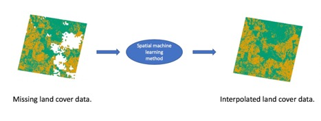
To meet the need for fast and accurate methods for interpolating missing data in satellite images, we present streamlined, fast, and accurate spatial machine learning methods to classify image features at the pixel level in satellite images with missing pixels. Our approach leverages key benefits of statistical machine learning methods for satellite imagery analysis: the ability to fit non-linear relationships, effectively cope with significantly large amounts of data, and high predictive accuracy [22]. We predict the values of pixels based on their spatial location in the image while using these methods.
We revisit the canonical geostatistical interpolation examples for satellite images that were previously explored by Pringle et al. (2009) [16] and Zhang et al. (2007) [23]. Due to the outlined challenges of implementing kriging and co-kriging for our application, we compare our methods with inverse distance weighted interpolation as an alternative well-established, accurate spatial interpolation method for remote sensing data. Inverse distance weighted interpolation uses spatial autocorrelation to interpolate unknown data by assigning more weight to the data closer to the observation of interest than data, which are geographically further away [24]. This method has been used for remote sensing data for decades [25] and with improvements in computing, it has recently been implemented for real-time analysis of sensor data [26].
The objective of our study is to spatially interpolate missing values due to cloud cover within satellite images and image products by using latitude and longitude as covariates, and statistical machine learning methods. Based on the results of the study, we describe some general rules for identifying when using these spatial machine learning methods will likely yield accurate results and be a useful alternative to image compositing.

2. Materials and Methods

2.1. Study Area

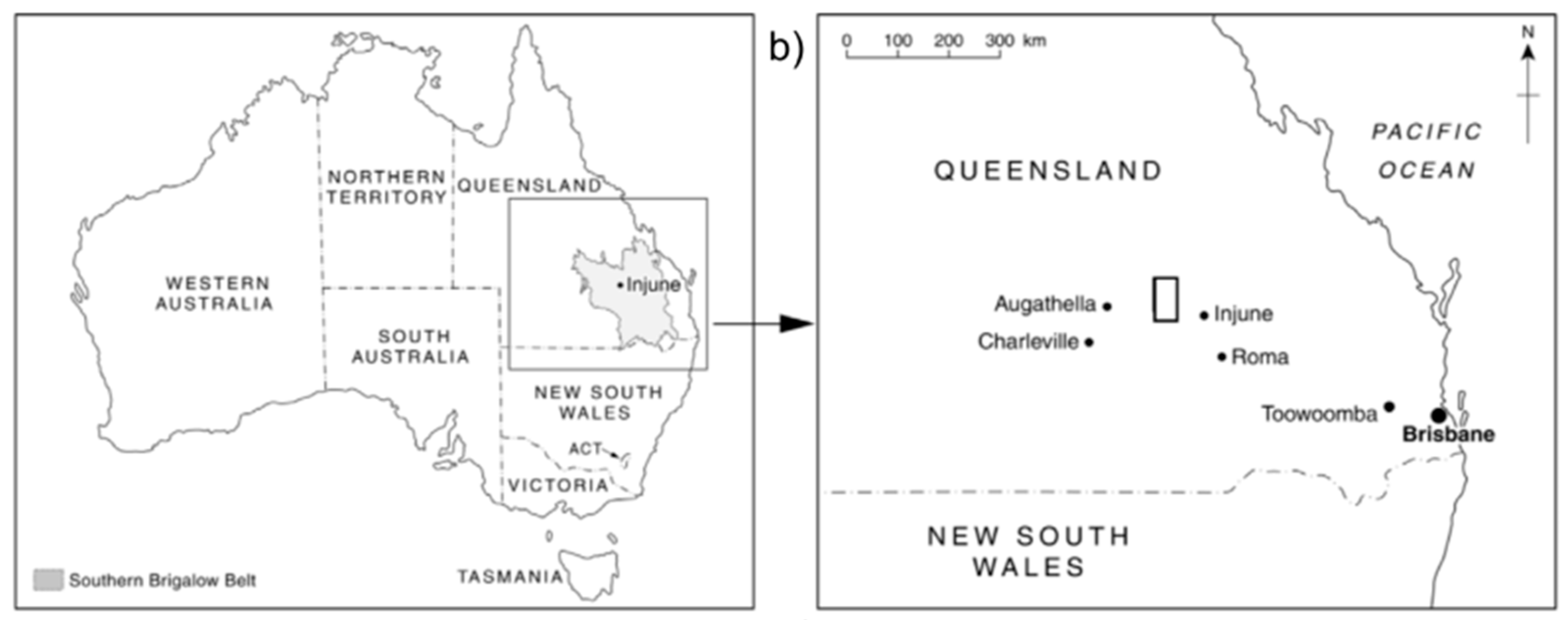
The study area is located approximately 100 km North West of the township of Injune in central southeast Queensland, Australia (see Figure 1). The landscape in the study area, which is 180 km × 180 km (one Landsat 7 scene), mainly consists of forest, pasture, and agricultural land, with some areas abandoned to revegetation [27]. Scattered buildings and unsealed roads are the main urban infrastructures present in the wider study area of Injune, however these are not present in the Landsat scene that was analysed [27].

2.2. Datasets

Our application requires a map of land cover for the study area. Spatial and Foliage Projective Cover (FPC) data that were based on Landsat 7 Thematic Mapper TM satellite images of the study area were provided by Queensland Department of Environment and Science [27]. FPC is defined as the vertically projected percentage cover of photosynthetic foliage or the fraction of the vertical view that is occluded by foliage [28]. We have selected this variable, because the presence and extent of woodland or forest is relevant to SDG 15, which focuses on forest management [29]. FPC can be manually collected in the field, however this is costly and time consuming, especially for large areas [28], and so, alternatively, FPC can be calculated at a large scale for entire satellite images. The image files were read into the software R as raster format images while using the Raster package [30]. From this data we extracted Foliage Projective Cover (FPC), latitude and longitude for each pixel.
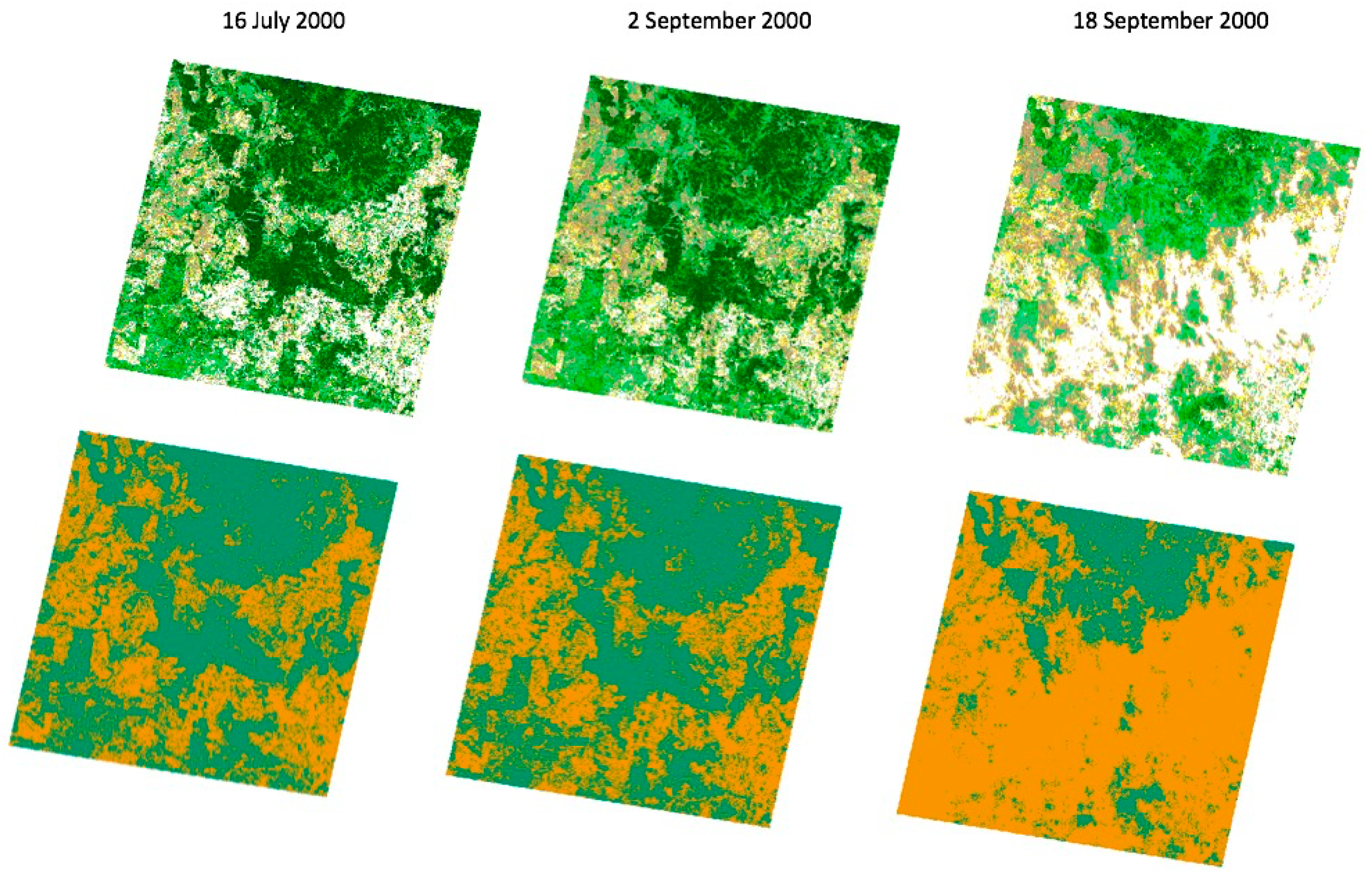
We then used the FPC value of each pixel to describe the land cover as either grassland or woodland (a binary categorical variable). FPC values from 0% to 15% were classified as grassland and from 16% to 100% were classified as woodland. In Queensland, Australia FPC above 10% is generally classified as woody vegetation [31], and we used a more conservative threshold of 15% that was based on advice of the FPC data provider, Queensland Department of Environment and Science. This binary categorisation of land cover was performed at the pixel scale for the entire images. We chose a binary land cover classification to simulate environmental monitoring, where binary information is required and useful, e.g., to differentiate between crop and not crop, forest and not forest, or species habitat or not. We use this simple binary land cover classification to explore the effectiveness of our methods at an uncomplicated level to demonstrate proof-of-concept. However, we also explore continuous values of FPC, which is a more complex landscape than the binary land cover classes.
FPC data were selected from July and September 2000 to examine how the models perform in different seasons (winter and spring, respectively, in Australia). Figure 2 shows the first two datasets have a mixture of woodland and grassland land cover, whereas the second spring dataset has noticeably more grassland land cover.
We first tested a simple scenario in which the majority of observations were one land cover class to explore the utility of our methods, and then explored more difficult cases where the land cover was heterogeneous. We intentionally selected a simulated dataset with a significantly higher proportion of grassland (18 September 2000). We chose this for proof of concept, because even if the models only predicted grassland, they would have high accuracy. If the models were unable to achieve high accuracy in this scenario, this would indicate other issues to explore in this approach. We also selected this dataset, because it approximates how a clearing event might appear in the landscape, with the sudden conversion of woodland to grassland, due to events such as intentional clearing for farmland, fire, etc. We used the results for this simple circumstance as the baseline for comparison with the more challenging scenario of a heterogeneous combination of two vegetation types, as seen in the 16 July and 2 September datasets.
We also examined whether converting FPC data to a binary classification before or after analysis made a difference to accuracy, in addition to examining whether the pattern of missing data affected the performance of the decision tree methods for predicting vegetation class and FPC value. To explore this, we trained the decision tree methods on continuous FPC values and predicted the continuous FPC values. Subsequently, we converted these continuous FPC values that were predicted by the models to a binary classification of grassland or woodland. We compared the accuracy of the converted FPC predictions with the accuracy of the predictions that were performed on FPC data, which had been converted to a binary classification of grassland and woodland prior to analysis.

2.3. Cloud Simulation

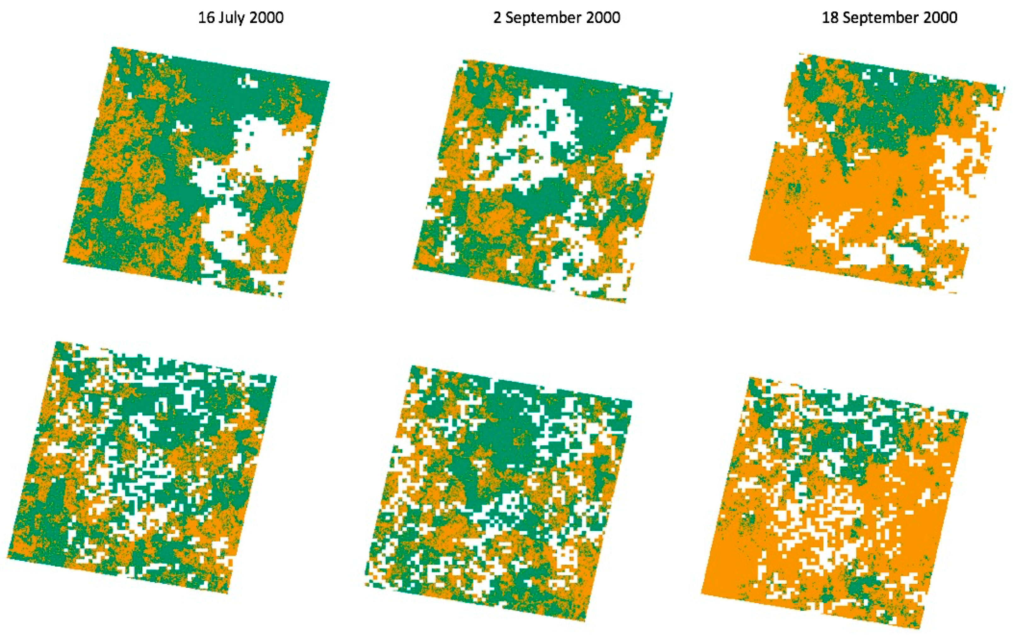
A simulated cloud mask was applied to random areas of the image to intentionally create ‘missing’ spectral data. The cloud-like shapes are simulated independently of the FPC data, while using a distance grid and applying a multivariate normal distribution, which is spatially autocorrelated with a covariance that exponentially declines with distance [32]. The simulated cloud layer was overlaid on the FPC layer and the corresponding pixels under the ‘clouds’ had their spectral information that was removed in the FPC layer. The large cloud shapes have more missing pixels adjacent to each other in clumps to simulate large and dense cloud cover and the small cloud shapes have missing pixels scattered across a wider area of the image to simulate thinner and dispersed cloud cover. Figure 3 shows plots of the images with simulated cloud patterns.

2.4. Methods Overview

We use machine learning methods to differentiate between two types of vegetation, namely grassland and woodland, and to predict the biophysical variable, Foliage Projective Cover (FPC), at the pixel level. We perform a simulation study to investigate the performance of our methods under different cloud patterns. A number of steps are required in order to perform the binary classification of grassland and woodland and FPC predictions. We show the overall process in Figure 4 and also describe it below.
First, we begin with a complete satellite image product of FPC, where no data are missing; that is, every pixel has an FPC value that is derived from satellite imagery, a binary classification as grassland or woodland, a latitude, and a longitude. We simulate cloud like shapes in an image layer, and delete spectral data in these regions of the satellite image, leaving only latitude and longitude information about these ‘missing’ pixels. This leaves the majority of the pixels in the image with both classification and spatial information (referred to as ‘observed pixels’), and a proportion of pixels with only spatial information where the cloud occludes any other data (referred to as ‘missing pixels’). We separately store the original FPC value and binary classification of the now-missing pixels, assume that these are the true values for the purposes of model testing, and use these as the ground truth to validate model performance in future steps.
Second, we take a random sample of the observed pixels we use to train the machine learning algorithms (see Figure 5). We randomly split this sample into a training set, containing 80% of the sampled pixels, and a testing set, containing 20% of the sampled pixels (see Figure 5). In the training set, the actual classification of the pixel (grassland or woodland) is retained, as is the continuous FPC value. In the testing set, the class and FPC of the pixel is removed, so it is unknown to the machine learning model. We run our decision tree machine learning models on the training sample to build a model that can predict whether the vegetation type of the pixels is grassland or woodland. Afterwards, in a separate test, the same method is used to build a model that can predict the continuous FPC value of missing pixels.
Third, after training, the machine learning models are used to predict the class of pixels in the testing set, which is a subset of the observed pixels (see Figure 4 and Figure 5). We produce confusion matrices and accuracy statistics based on the results of predicting the class of pixels in the testing set to assess the predictive accuracy of the models. This allows for us to verify the effectiveness of the models for predicting the values of pixels missing due to cloud cover.
Fourth, the resulting models are then used to interpolate the land cover classification of any pixels missing in the image. We compare these to the ‘ground truth’ data that we stored earlier to evaluate the overall accuracy of our interpolation method, and therefore evaluate whether our proposed methods are useful, fast, and accurate.
We perform this training, testing, and accuracy assessment process on two random samples of observed pixels and two random samples of missing pixels per image with each of the different cloud patterns (six images and 24 samples) and implement both the gradient boosted machine and random forest algorithms. We apply this approach for both a binary classification of FPC and prediction of continuous FPC values.
We examine and compare the performance of two types of decision tree machine learning methods (in steps two and three above) in our study. They both use many simple decision trees to classify observations, however the algorithms combine them in different ways to reach final classifications and predictions. We compare the results of the decision tree methods with inverse distance weighted interpolation, which is an established, known interpolation method for remote sensing data. The methods will be described in more detail in Section 2.5 and Section 2.6.
A key benefit of the decision tree methods is that they only require a relatively small amount of the total data available to be effectively trained and perform accurate classifications. Even with data missing due to cloud cover, satellite images will have millions or billions of pixels that are available for training, and training on only thousands of pixels can produce accurate models for classifying the unknown test data.

2.5. Decision Tree Methods

Statistical machine learning methods, which are also called artificial intelligence methods, use algorithmic models to analyse data. These methods treat the way in which the data were generated or relationships between the variables as unknown [33]. Decision trees are a category of machine learning methods that can be used to classify large amounts of data [34]. Decision trees are first trained on data where the values of the observations are known, and are then used to predict the values of observations in the testing data, where the values of the observations are unknown.
Decision tree methods can be applied to large amounts of data due to their computational simplicity, which is useful for satellite imagery analysis that is performed on thousands or millions of pixels. Examples of the use of decision trees in the remote sensing literature include identifying land cover [35], mapping forest change globally [36], and identifying land use classes, such as agriculture, built up areas, and water in Surat city, India [37]. However, decision tree methods in their simple form are prone to inaccuracy [34]. It is very difficult, if not impossible, to accurately classify observations that are based on only one decision rule. For example, classifying pixels as bare earth or forest based on the value of only one variable would lead to very inaccurate results. By combining many simple decision trees, decision tree algorithms gradient boosted machine and random forest can perform highly accurate classifications. In our study, we compare the performance of these two popular types of decision tree methods.

2.5.1. Gradient Boosted Machine

Gradient boosted machine is a type of boosted decision tree method, which is configured to avoid the accuracy issues that are associated with simple, single decision trees [34]. Boosting is the concept that it is easier to find and average many inaccurate or ‘weak’ decision rules than to find one that is highly accurate [22]. A gradient boosted machine has three key components: a simple decision tree, also called a weak learner, a loss function, and an additive model. A weak learner is a simple decision tree, which, if used on its own, would predict the class of observations with low accuracy. Using boosting, decision trees are iteratively fit to training data, while using multiple weak learners to classify observations, gradually emphasising observations modelled inaccurately by the previous collection of trees. By focusing on the variability in the data unexplained by previous trees, with each new tree that is fit the variance, or error, is further reduced. This iterative minimisation of the loss function is the ‘boosting’ approach, and it is also called the gradient descent procedure, which is where the method gets its name [22]. The loss function of a gradient boosted machine is given by
F * ( x ) = arg   min F E y , x   L ( y ,   F ( x ) )
where x is a covariate, y is the dependent variable, and F * is a single decision tree function mapping covariate observation x to dependent variable y [38]. The gradient boosted machine uses the training data to estimate a decision tree that will accurately predict the class of observations, while minimising the expected value of the loss function L ( y ,   F ( x ) ) over the joint distribution of all the dependent variable and covariate values [38]. Different loss functions can be chosen, and in this study, we choose the squared error loss function ( y F ( x ) ) 2, because it is effective and commonly used [38]. This is also the default in the gbm package [39] we used to fit the gradient boosted machine in the case study.
For a gradient boosted machine, as defined by [38], each decision tree is expressed
h ( x ;   { γ j ,   R j } 1 J ) = j = 1 J γ j 1   ( x R j )
That is, the gradient boosted machine h ( x ) is a combination of multiple weak learners ( F * in Equation (1)). γ j is a constant value that is used as a threshold to split the observations into different classes. Depending on where an observation’s value j for variable R compares with the constant value, γ j , the observation will either be placed into a final classification (terminal node) γ j or continue to be analysed based on other γ j values until a final classification is reached for that observation. The indicator function has the value 1 if the decision tree argument is true, e.g., the value of observation R j < γ j and zero if it is false. These functions allow for the gradient boosted machine to classify observations while using many decision trees to reach a final classification. The variables   R that determine how observations are separated into different classifications and the values of those variables j that represent the splits at non-terminal nodes in the tree are represented as { R j } 1 J .
The gradient boosted machine in our study is a combination of many weak learner decision trees that are fit to minimise the loss function, ( y F ( x ) ) 2 at each iteration, which as defined by [38], can be expressed as:
          T ( x ) = ( y j F ( x ) ) 2 + j = 1 J γ j 1   ( x R j )
Each new decision tree is fit to the covariates in a way that reduces the loss function, ( y j F ( x ) ) 2 . This reduction at each iteration of the algorithm approximates the gradient of the decrease in loss function that is necessary to improve the fit of the model to the data [39]. Latitude and longitude are included as covariates R in our spatial gradient boosted machine.

2.5.2. Random Forest

The random forest algorithm is a decision tree method that uses bagging in order to reduce variance by averaging many inaccurate but approximately unbiased decision trees [34]. Bagging is similar to boosting, in that it combines many weaker rules rather than using one decision rule, but boosting produces a sequence of weak decision rules and bagging takes an average [22].
A random forest draws a bootstrap sample Z * of size N from the training data to grow a decision tree, T b to the data. The trees are created by repeatedly and randomly selecting the m variables from the potential set of p variables, choosing the variable that best separates the data into two groups [34]. This process is repeated to grow a forest of these decision trees classifiers expressed by [34] as
{ T b } 1 B
Each observation x is classified not by just one of these trees, but by the forest of individual trees. This means each observation is classified based on what the majority of the decision trees predict. This can be expressed as
C ^ r f B ( x ) = m a j o r i t y   v o t e   C ^ b { ( x ) } 1 B
where C ^ b ( x ) is the class prediction of the b th random forest [34]. In our spatial random forest, the latitude and longitude are included as covariates p which are randomly selected as m variables to grow the random forest classifiers in the final ensemble { T b } 1 B and to classify observations.

2.5.3. Tuning Parameters and Computation

Tuning parameters can be set to change the running and performance of machine learning algorithms. For decision tree methods generally, we can choose different values of tuning parameters, such as the number of trees, learning rate, and interaction depth. The number of trees specifies how many simple decision trees will be fit by the algorithm, learning rate specifies the contribution of each individual tree to the overall model, and the interaction depth specifies how many interactions are fit (one way, two way, etc.) [34]. The investigation and explanation of optimal values for these parameters is an entire body of research itself beyond the scope of this work (see Elith et al. (2008) [34]). In this paper, we implement the gradient boosted machine and random forest algorithms based on recommendations from Elith et al. (2008) [34], which in some cases are also the default values in the software packages that we use.
The gradient boosted machine models were fit while using the R package ‘gbm’ [40]. The tuning parameters, number of trees, shrinkage parameter (also known as the learning rate), and interaction depth, were set using rule of thumb values that were specified by [22]. The random forest models were fit using the package randomForest [41]. We implement the inverted distance weighted interpolation method using the package gstat [42] in R.

2.6. Samples, Accuracy Measurements

The random forest, gradient boosted machine, and inverse distance weighted interpolation methods were trained on samples of 8000 pixels in the satellite image, and predictions were made on 2000 pixels each time (an 80%/20% training and testing data split [34]). In the training sets the proportion of grassland ranged from 31–38%, 34–36%, and 61–78% for the 16 July, 2 September, and 18 September 2000 data, respectively. The proportions were the same in the testing set, except the 18 September 2000 data grassland ranged from 61–71%. The proportion of woodland in the training sets ranged from 62%–66%, 64–66%, and 22–37% for the 16 July, 2 September, and 18 September 2000 data, respectively. In the testing sets, the proportion of woodland ranged from 62–69%, 64–66%, and 22–39% for the 16 July, 2 September, and 18 September 2000 data, respectively.
The accuracy of the methods was assessed while using overall accuracy, producer’s accuracy, and user’s accuracy statistics produced from confusion matrices for binary classification of vegetation type. Producer’s accuracy (which is related to omission error) is the probability the observation in the data is classified as the same class and user’s accuracy (which is related to commission error) is the probability the classified observations are the same class in the reference data [
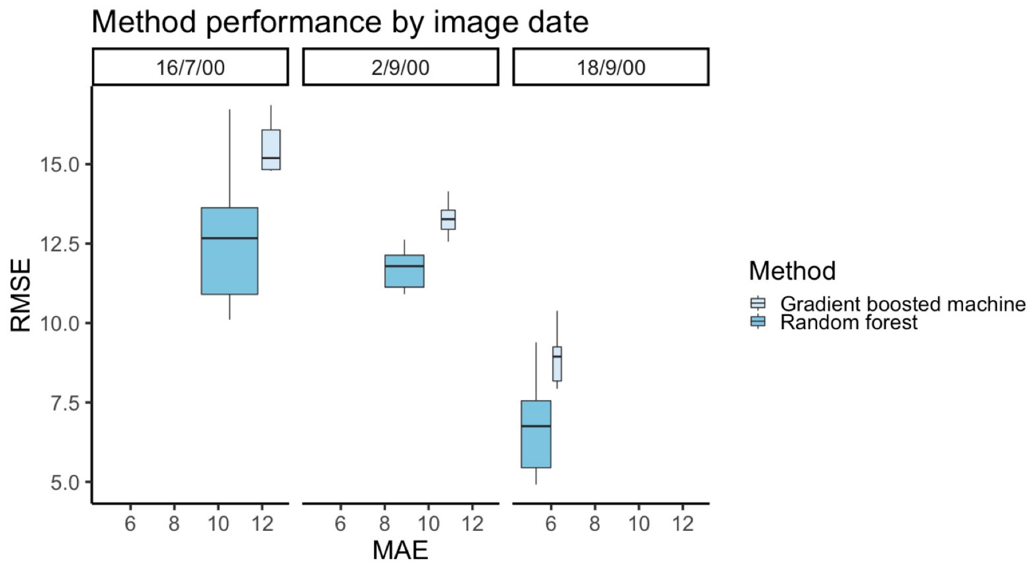
43]. The accuracy of the methods for the prediction of continuous FPC values was assessed while using root mean squared error (RMSE) and mean absolute error (MAE). Root mean squared error is calculated by taking the average of the squared model residuals, and then taking the square root of this average [44]. The mean absolute error is the average of the residuals i.e., the average of the difference between the predicted and observed values [45]. The overall, producer’s, and user’s accuracy statistics were produced while using the caret package [46] in R.
We performed one-way ANOVA tests. ANOVA tests identify differences between group means, and whether these differences are statistically significant or not to identify differences in mean overall accuracy and RMSE between groups based on methods, pixel class (missing or observed), image dates, and cloud pattern (small or large) [47]. We report the F statistic and the corresponding p-value [47]. We also present Tukey post-hoc test results [47] to identify significant pairwise differences between groups. These statistics were produced in base R while using the ‘aov’ function.

3. Results

3.1. Classifying Binary FPC: Woodland and Grassland

For binary classification of pixels in the images, random forest had higher accuracy than gradient boosted machine across all image dates for both missing and observed pixels. These results are reflected in Figure 6, as the random forest results were more accurate than the gradient boosted machine when compared by cloud pattern and by pixel class.
Random forest was consistently more accurate across the image dates, as shown in Figure 7. Gradient boosted machine and random forest both had the highest accuracy for the 18 September 2000 image, which had the highest prevalence of one class; grassland. This result met our expectations, since most of the observations in the image are grassland. For the more heterogeneous images on 16 July 2000 and 2 September 2000, the methods also had high accuracy, particularly the random forest.
Although the majority of the pixels in the simple circumstance, the 18 September 2000 image, were grassland, the models also predicted woodland observations, and correctly in most cases. To illustrate, here we present the producer’s and user’s accuracy results for the most accurate algorithm, random forest, for both missing and observed pixels for the 18 September 2000 image in Table 1.
Although most of the training and testing data are grassland in this simple circumstance, the random forest is able to predict both grassland and woodland with a relatively low number of incorrect classifications. The algorithm predicts grassland more accurately than woodland from both the producer’s and user’s perspective, and this meets our expectations, given the high prevalence of this class in the image. We present these results to show the model did predict woodland accurately, despite the high proportion of grassland in the data.
Table 2 shows that random forest had the highest accuracy overall when compared with the gradient boosted machine. The highest accuracy results, on average, for the random forest were for the missing pixels in the small cloud pattern (Overall accuracy = 0.869) and missing pixels in large cloud pattern (Overall accuracy = 0.864) in the 18 September 2000 image, followed by observed pixels in the same image. The lowest accuracy results on average for random forest for binary FPC classification were for missing pixels in the 16 July 2000 and 2 September 2000 images, which have more balanced class groups than the 18 September 2000 image. The lowest accuracy result was for missing pixels in a large cloud pattern in the 2 September 2000 image (Overall accuracy = 0.729) and for missing pixels in the large clouds pattern in the 16 July image (Overall accuracy = 0.749). Random forest had overall accuracy between 0.75 and 0.87 for classifying missing pixels and between 0.76 and 0.86 for classifying observed pixels based on the average results across multiple samples.
Table 3 shows gradient boosted machine had the highest accuracy results on average for missing pixels in the 18 September 2000 image for both the small cloud pattern (Overall accuracy = 0.827) and large cloud pattern (Overall accuracy = 0.815). The method also performed well at classifying the observed pixels in the 18 September 2000 image for both the large cloud pattern (Overall accuracy = 0.812) and small cloud pattern (Overall accuracy = 0.796). Gradient boosted machine also had high accuracy for the 16 July image for missing pixels in the small cloud pattern (Overall accuracy = 0.736) and observed pixels in the image (Overall accuracy = 0.717). The lowest accuracy result was for the 16 July image for the missing pixels in the large cloud pattern (Overall accuracy = 0.675), followed by observed pixels for the same image (Overall accuracy = 0.682). Based on the average results across multiple samples, the gradient boosted machine had an overall accuracy between 0.67 and 0.83 for classifying missing pixels and between 0.68 and 0.81 for classifying the observed pixels.
For both gradient boosted machine and random forest, the highest accuracy result was for missing pixels due to the small cloud pattern in the 18 September image. This is contrary to expectations, because the methods generally perform better on the observed pixels. This result could be due to the higher prevalence of grassland in this simple circumstance image, or due to sampling coincidentally aligning with the balance of the classes in the missing pixels for that image. More accurate performance classifying missing pixels did not present as a trend in the results overall.
Table 4 shows there was a significant difference between overall accuracy of gradient boosted machine and random forest methods, according to a one-way ANOVA (F = 16.650, p < 0.0001, and image date (F = 31.411, p < 0.0001). There was a significant difference between the 18 September 2000 image and 16 July 2000 image (p < 0.0001) with mean overall accuracy 0.094 higher for the 18 September 2000 image according to a one-way ANOVA. There was a significant difference between the 2 September 2000 and 18 September 2000 images, with mean overall accuracy of 0.095 lower for the 2 September 2000 image.
There was no significant difference between the 16 July 2000 and 2 September 2000 images (p = 0.9927), or between the mean overall accuracy of the methods and pixel class (F = 0.003, p = 0.957) or cloud pattern (F = 0.1745, p = 0.6782), according to a one-way ANOVA. There was no significant interaction between overall accuracy, method, and image date according to a two-way ANOVA (F = 1.2469, p = 0.2978). There was also no significant interaction between overall accuracy, pixel class, and cloud pattern, according to a two-way ANOVA (F = 2.1925, p = 0.1458). Additional tables of ANOVA results are in the Supplementary Materials.

3.2. Predicting Continuous FPC

For continuous FPC prediction, random forest had lower error statistics than the gradient boosted machine across all images for both missing and observed pixels (Figure 8). The random forest results were more accurate (had lower error rates) than the gradient boosted machine when compared by pixel class and cloud pattern.
As expected, both the gradient boosted machine and random forest were the most accurate for the 18 September 2000 image, with the lowest RMSE and MAE. The methods also had high accuracy for the heterogeneous images, 2 September 2000 and 16 July 2000, but they were the least accurate for the July 2000 image. This is reflected in the plots in Figure 9.
The FPC values in the testing samples for continuous FPC ranged from 0% to 75.2% for the 16 July 2000 image, 0% to 66.9% for the 2 September image, and 0% to 78.58% for the 18 September 2000 image. In addition to RMSE and MAE statistics, we present these error measurements as a percentage of mean FPC. In the tables, we present averages across samples for cloud pattern and pixel class. The full results per sample are in the Supplementary Materials.
Table 5 shows when predicting FPC values random forest had an average RMSE ranging from 5.118 to 13.871, with lower RMSE values indicating more accurate performance and higher RMSE values indicating less accurate performance. Random forest consistently had the lowest average RMSE values (i.e., was more accurate) for the 18 September 2000 image (RMSE = 0.5118 to 7.608) when compared with the 2 September 2000 image (RMSE = 10.917 to 12.556) and the 16 July 2000 image (RMSE = 10.962 to 13.871). The lowest average RMSE across samples was for missing pixels in the small cloud patterns for the 18 September 2000 image (RMSE = 5.118, MAE = 3.807), followed by observed pixels in the large cloud pattern image (RMSE = 7.001, MAE = 4.598) and missing pixels in the large cloud pattern (RMSE = 7.440, MAE = 5.491) for the same image date. The highest average RMSE (i.e., least accurate) results was for predicting continuous FPC values in the 16 July 2000 image for missing pixels in the large cloud pattern (RMSE = 13.871, MAE = 11.098), followed by observed pixels (RMSE = 13.631, MAE = 9.758) and missing pixels in the small cloud pattern (RMSE = 12.080, MAE = 9.518) for the same date.
Table 6 shows when predicting FPC values gradient boosted machine had an average RMSE that ranged from 9.65 to 16.09. Gradient boosted machine had the lowest RMSE (i.e., highest accuracy) for the 18 September 2000 image for missing pixels in the small cloud pattern (RMSE = 9.646, MAE = 7.065), followed by missing pixels in the large cloud pattern (RMSE = 8.658, MAE = 6.772) for the same image. The method consistently performed accurate classifications for both missing and observed pixels in the 18 September 2000 image. The highest average RMSE (i.e., lowest accuracy) was for predicting FPC for missing pixels in the small cloud pattern in the 16 July 2000 image (RMSE = 16.091, MAE = 12.872), followed by missing pixels in large cloud pattern (RMSE = 15.849, MAE = 13.352) and missing pixels in small cloud pattern (RMSE = 15.108, MAE = 12.855) for the same image. Gradient boosted machine performed the least accurate classifications of continuous FPC on average for the 16 July 2000 image.
Table 7 compares the performance of the inverse distance weighted interpolation and random forest methods. Overall, the random forest consistently had higher accuracy (lower RMSE and MAE) than inverse distance weighted interpolation across all images and cloud patterns for both missing and observed pixels. When predicting continuous FPC values, the inverse distance weighted interpolation had an average RMSE that ranged from 7.33 to 16.45. This method performed the best for classifying large cloud patterns in the 18 September 2000 image for missing pixels in the large cloud pattern (RMSE = 7.514, MAE = 5.126), the worst for classifying large cloud pattern for the 16 July 2000 image (RMSE = 16.200, MAE = 13.795). The improvement in accuracy was more noticeable for the missing pixels. For random forest, the gradient boosted machine and inverse distance weighted interpolation the methods had the highest accuracy for the 18 September 2000 image for both binary classification and prediction of FPC values. This image has a majority of grassland class pixels.
Table 8 compares the performance of the inverse distance weighted interpolation and gradient boosted machine methods. Overall, inverse distance weighted interpolation had higher accuracy (lower RMSE and MAE) than gradient boosted machine across all images and cloud patterns for both missing and observed pixels. Table 6 and Table 7 show overall random forest had the highest accuracy for continuous FPC prediction (RMSE from 5.118 to 13.871), followed by inverse distance weighted interpolation (RMSE from 7.541 to 16.200), and gradient boosted machine was the least accurate of the three methods (RMSE from 8.072 to 16.091).
Table 9 shows that there was a significant difference between at least two of the three methods (F = 6.128, p = 0.004), according to an ANOVA. A posthoc Tukey test showed a significant difference between gradient boosted machine and random forest (p = 0.029) with mean RMSE for random forest 2.174 lower than for gradient boosted machine. ANOVA showed a significant difference in mean RMSE between inverse distance weighted interpolation and gradient boosted machine (p = 0.004), with mean RMSE 2.754 lower for inverse distance weighted interpolation. There was no significant difference between random forest and inverse distance weighted interpolation for predicting continuous FPC.
There was a significant difference in mean RMSE between at least two image dates (F = 59.65, p < 0.0001). A Tukey posthoc test showed that there were significant differences between the 16 July 2000 and 18 September 2000 images (p < 0.0001), with a mean RMSE 5.732 lower for the 18 September 2000 image. There was a significant difference in mean RMSE between the 2 September 2000 and 18 September 2000 images (p < 0.0001) with mean RMSE 4.247 higher for 2 September 2000. There was no significant difference between the 16 July 2000 and 2 September 2000 images (p = 0.0219). The results also showed there was no significant difference between RMSE of methods and pixel class (F = 2.068, p = 0.155) or cloud pattern (F = 0.109, p = 0.742). Additional ANOVA results tables are in the Supplementary Materials.

3.3. Converting Predicted FPC to Binary Classification: Woodland and Grassland

We found that the conversion of continuous predictions of FPC to a binary classification after analysis created a substantial loss of accuracy for both the random forest and gradient boosted machine methods. This was particularly noticeable for gradient boosted machine models. In this study, the random forest and gradient boosted machine methods produced more accurate predictions of binary land cover type when the class variable was derived prior to analysis, rather than producing a continuous FPC prediction and then converting these results to a binary classification.
To examine whether predicting continuous FPC values and then converting these to a binary classification, rather than recoding FPC to a binary classification prior to analysis affected the accuracy of the methods we compared results for both approaches for the 2 September 2000 image. This image has a relatively heterogenous landscape that is made up of both woodland and grassland pixels.
For random forest, we observed a noticeable reduction in overall accuracy from an average range of 0.74 to 0.77 for binary classification down to 0.66 to 0.70 by converting continuous FPC value predictions to a binary variable after initial analysis (see Table 10). These results indicate a substantial reduction in model accuracy as a result of converting a continuous FPC prediction to binary after analysis, rather than performing the conversion to a binary variable prior to performing analysis.
Table 11 shows for gradient boosted machine we also found a substantial reduction in overall accuracy, from an average range of 0.71 to 0.75 to 0.66 to 0.70 by converting continuous FPC value predictions to a binary variable after initial analysis.
Inverse distance weighted interpolation is not able to perform categorical classifications directly, so all of the results were predicted as continuous FPC first and then converted to the binary class variable to produce confusion matrix results. This means that it is not possible to compare converted results with the results of binary classifications that were performed by inverse distance weighted interpolation, as was done for gradient boosted machine and random forest in Table 9 and Table 10. A table of results for inverse distance weighted interpolation for all of the samples is available in the Supplementary Materials (Table S14). Table 8 shows converted overall accuracy of inverse distance weighted interpolation ranged from 0.64 to 0.85 on average. Binary classification accuracy for inverse distance weighted interpolation was compared with random forest because it was the most accurate of the two decision tree methods in this case study. Table 12 shows random forest consistently had higher overall accuracy on average than converted inverse distance weighted interpolation, with the overall accuracy ranging from 0.75 to 0.87. Random forest also had consistently higher accuracy than inverse distance weighted interpolation for prediction of continuous FPC, as measured by RMSE and MAE.

4. Discussion

Monitoring progress towards the Sustainable Development Goals (SDGs) provides important insights into the state of the environment and quality of human life in countries, but the cost of collecting data is a barrier to measuring the SDGs. Free satellite images are a key data source to overcoming this barrier, however there are associated quality issues with these images due to missing data from cloud cover, especially in tropical areas. We have presented streamlined spatial machine learning methods that can fill gaps in satellite images due to missing data to address this challenge, and classify pixels into different vegetation types to identify grassland and woodland.
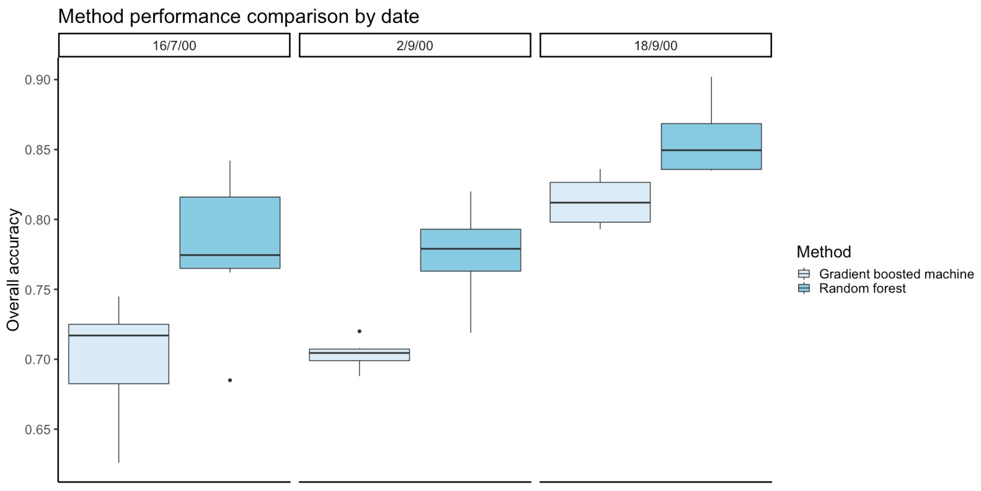
The spatial gradient boosted machine and random forest methods produce fast and accurate predictions (overall accuracy between 0.63 and 0.90) of pixel class over entire images for both the observed and missing pixels. Overall, random forest had higher accuracy for performing binary classification of pixels and predicting FPC values than gradient boosted machine without an increase in computation time. Of the decision tree models, we would recommend using the random forest rather than gradient boosted machine for binary image classification and continuous variable prediction tasks. Random forest also had consistently higher accuracy for performing prediction of continuous FPC values than inverse distance weighted interpolation across all images, cloud patterns, and pixels classes. This held true for both prediction of continuous FPC values and binary classification of pixels as grassland or woodland. Inverse distance weighted interpolation had consistently higher accuracy than gradient boosted machine for predicting continuous FPC. Overall, random forest was the most accurate of the three methods for binary classification and FPC prediction.
This accurate binary classification was achieved by converting continuous FPC values into binary classes from the outset, and then using the decision tree methods to predict a binary classification. Changing that order by predicting continuous FPC using the methods and then converting to a binary classification was substantially less accurate for both decision tree methods. This loss of accuracy was worse for the gradient boosted machine. We recommend transforming from a continuous value to binary classification prior to analysis and training the methods on the binary classification problem rather than converting continuous predictions to binary classifications after initial analysis.
The binary land cover classification that we performed in the case study show the methods perform well in a simple case, however land cover maps are usually more detailed and extensive in terms of number of categories and the scale e.g., detailed classifications at state or country level. In future work, it would be of interest to explore how the methods perform in a scenario with more land cover classes, particularly because the methods perform well at the more complex task of predicting continuous data.
Counterintuitively, the accuracy of image classification was not impacted by size of the clouds; we did not identify a clear pattern where the models identified pixels in the small cloud pattern more accurately than the large cloud pattern. Rather, the land cover heterogeneity seemed to influence model performance more than the pattern of the simulated clouds. The gradient boosted machine and random forest both had highest accuracy for binary classification when identifying missing pixels in the 18 September 2000 image, which had more grassland. Overall, random forest had higher accuracy for performing binary classification of pixels than gradient boosted machine.
While there are many benefits to the decision tree methods, as with any statistical method it is important to be aware of and address issues, such as overfitting and bias/variance tradeoff. It is noted that the boosting and bagging aspects of the gradient boosted machine and random forest algorithms that were adopted in this paper are designed to address these issues [34,38]. In our analyses, the decision tree methods were demonstrated to achieve high accuracy for both training and test data, indicating good fit and an acceptable bias/variance balance. This engenders confidence in the ability of the models to adequately predict missing data that were generated by cloud cover in the case study.
Another issue is training and testing sample selection for both observed and missing pixels. If there is a class imbalance in the image, such as more grassland in the missing pixel region and the randomly selected training set includes mostly or only woodland pixels, the trained method might be more likely to incorrectly classify the test set as woodland. A potential solution could be to select a training set deliberately from a region of the image with a combination of the classes you want to predict, however this may also introduce bias to the model. In this study, we simulated the clouds so knew what the true classifications were in the image, however this will not be so in real cases of missing data due to cloud cover. In cases where there is a class imbalance in the image and the methods produce inaccurate results due to lack of balanced training data, while using the composite approach for interpolation may be more appropriate.
In the case where large amounts of spectral data are missing from images over long periods of time, such as most of the year in the tropics [12], the use of our methods can provide fast results to a level of accuracy that can be practically useful for informing decisions, even with a more heterogenous landscape (minimum 0.60 overall accuracy for binary classification) or highly accurate results for images with a higher prevalence of one class (up to 0.90 overall accuracy). Of course, there is error that is associated with model derived estimates, so confidence intervals should be considered and any additional available data or local knowledge when interpreting the results.
In this scenario, because we simulated missing data, we were able to validate the predictions that the methods produced, because we had the “true” value of the pixels. However, in the case where the true values of the pixels are unknown, this will not be possible for the testing data which are being classified. This is not an argument against using statistical methods to interpolate missing values when the data are truly missing. Rather, it is a caution to keep in mind that there will be uncertainty regarding the land cover classifications, as there is in any model, and hence to consider the confidence intervals around the model predictions.
Our application of these methods was motivated by considering what agencies and developing countries can achieve with a minimum core set of free resources to perform analyses in operational programs to gain insights into their environment and contribute to monitoring environmental SDGs. We describe three core free resources to monitor environmental SDGs. First, free satellite images and satellite image derived data products. These images can be downloaded for free from a number of sources, including CEOS Data Cube products [8] and the USGS Global Visualization Viewer [9], or Google earth engine [48]. These are only a selection of products currently available, and many more resources are being produced and shared over time. Second, free open source software products with online resources and communities can be used to produce estimates of the SDGs, and indeed other statistics. Here, we used R software [49]. Third, spatial information (i.e., latitude and longitude) can be extracted from any satellite image at no cost using code in open source software. The latitude and longitude of an image will remain intact, regardless of whether the spectral information associated with those pixels exists. Through our case study, we have shown by using these three free resources, measuring selected SDGs which are observable directly or by proxy from satellite images as accurately is possible, which offers opportunities to measure SDGs effectively, even in regions where missing data due to cloud cover or limited available infrastructure or funding to collect data are issues.
Our intention in describing and demonstrating the use of these free resources is not to prescribe the best practice or most accurate resources and methods for measuring SDGs or to dismiss directly collected data or more complex methods. Rather, the intention is to provide a streamlined path to monitoring SDGs in a tangible and fast manner, while still providing reasonable accuracy. By using these three minimum resources, this is achievable. Although the inclusion of auxiliary variables was not explored in this study, it is noted that as with any statistical model including informative covariates will improve the classification accuracy of the proposed methods. Here, we have presented the minimum core resources to measure selected environmental SDGs while only using free resources and streamlined methods.
Here, we explored the use of latitude and longitude as covariates in decision tree methods to classify pixels into different types of land cover as relevant to environmental SDG 15 life on land; specifically forest cover monitoring and deforestation detection [6]. We focused on this SDG in our approach, and our methods are specifically useful for contributing to:
SDG Indicator 15.1.1 Forest area as a proportion of total land area; and,
SDG indicator 15.3.1 Proportion of land that is degraded over total land area.
These methods may aid in the monitoring of different SDGs which are also measurable from satellite images, such as identifying bodies of water, level of sediment in water sources, presence of crop land, and other environmental features. Further investigation could also be done into the application of these spatial methods to predicting satellite image spectral band values directly, rather than products that are derived from the spectral band values, such as FPC.

5. Conclusions

The Sustainable Development Goals (SDGs) are important indicators of quality of human life and the environment, which are a priority for countries to progress towards meeting by 2030. Some key barriers to monitoring the SDGs include the cost of acquiring and collecting data, lack of infrastructure, and required skills within countries and organisations to produce statistics from satellite imagery data [10]. Satellite imagery is a useful, freely available data source that can directly contribute to monitoring and measuring the SDGs [2,4,5] and it addresses the issue of cost of data acquisition. However, missing data due to cloud cover and ways to fill in these gaps as effectively as possible are issues with these images, especially in tropical regions of the world.
We have presented two fast and accurate spatial machine learning methods that meet the need for effective ways to fill gaps in images due to missing data, and produce statistics to monitor indicators of SDG 15; life on land, related to forest management. The results showed our random forest method was more accurate than inverse distance weighted interpolation for predicting Foliage Projective Cover (FPC) for missing and observed data across all images in the study. Our methods are implemented in free software, performing binary classification of both observed and missing pixels into vegetation classes; woodland and grassland, and predicting continuous FPC values. These accurate classifications are possible using only latitude and longitude of the pixels as covariates, which can be extracted from any satellite image, regardless of cloud cover. We have provided some general rules of thumb for when our approach would be most useful, and recognise cases when an alternative, such as the traditional compositing approach, may be more suitable for filling in image gaps due to limitations of our approach.
Our methods are effective for contributing to SDG 15 related to forest management, and importantly could also be applied to other environmental SDGs identifiable in satellite images, such as SDG 6: Clean sanitation and water through water quality and water extent, and SDG 2: end hunger by identifying crop type and crop area. By using these methods and the core set of minimum free resources, we describe satellite images, software, methods, and spatial information; it is possible for other users and countries to effectively monitor and model environmental SDGs, importantly at low cost in terms of finances, infrastructure, and experience working with satellite imagery data.

Supplementary Materials

The following are available online at https://www.mdpi.com/2072-4292/11/15/1796/s1, Table S1: Random forest binary classification results by image date, ordered from highest overall accuracy to lowest for each date, Table S2: Gradient boosted machine binary classification results by image date, ordered from highest overall accuracy to lowest for each date, Table S3: Binary FPC Anova results. Tukey posthoc comparison results showing differences in mean overall accuracy between image dates. Table S4: Binary FPC Anova results. Tukey posthoc comparison results showing differences in mean overall accuracy between image dates, Table S5: Two-way ANOVA results for differences in mean overall accuracy for binary FPC. Table S6: Random forest continuous FPC prediction results ordered by image date, from lowest root mean squared error (RMSE) to highest for each date, Table S7: Gradient boosted machine continuous FPC prediction results ordered by image date, from lowest root mean squared error (RMSE) to highest for each date, Table S8: Continuous FPC ANOVA results. Tukey posthoc comparison results showing differences in mean RMSE between image dates, Table S9: Continuous FPC ANOVA results. Tukey posthoc comparison results showing differences in mean RMSE between methods, Table S10: Two-way ANOVA results for differences in mean RMSE for continuous FPC, Table S11: Random forest accuracy results for continuous FPC predictions converted to binary class after analysis, Table S12: Gradient boosted machine accuracy results for continuous FPC predictions converted to binary class after analysis. Table S13: Inverse distance weighted interpolation method continuous FPC prediction results ordered by image date, by cloud pattern and pixel class for each date. Table S14. Inverse distance weighted interpolation method accuracy results for converted continuous FPC predictions to binary classification by image date, by cloud pattern and pixel class for each date.

Author Contributions

J.H. conceived and wrote the paper, with input from K.M., K.J.H. and M.S., M.S. provided satellite images. J.H. performed simulations and analysed the data.

Funding

This research received no external funding.

Acknowledgments

The authors would like to thank the Queensland Department of Environment and Science for providing data for this project. The authors thank Matthew Pringle, Bulukani Mlalazi, Charles T. Gray, Alan Pearse and Miles McBain for useful discussions and advice on code.

Conflicts of Interest

The authors declare no conflict of interest.

References

  1. United Nations. Sustainable Development Goals: Sustainable Development Knowledge Platform. Available online: https://sustainabledevelopment.un.org/?menu=1300 (accessed on 29 June 2018).
  2. GEO Earth Observations and Geospatial Information: Supporting Official Statistics in Monitoring the SDGs. 2016. Available online: http://www.un.org/ga/search/view_doc.asp?symbol=A/RES/70/1&Lang=E (accessed on 7 July 2018).
  3. United Nations United Nations Global Working Group on Big Data for Official Statistics. Available online: https://unstats.un.org/bigdata/ (accessed on 10 April 2018).
  4. Anderson, K.; Ryan, B.; Sonntag, W.; Kavvada, A.; Friedl, L. Earth observation in service of the 2030 Agenda for Sustainable Development. Geo Spat. Inf. Sci. 2017, 20, 77–96. [Google Scholar] [CrossRef]
  5. Holloway, J.; Mengersen, K. Statistical Machine Learning Methods and Remote Sensing for Sustainable Development Goals: A Review. Remote Sens. 2018, 10, 1365. [Google Scholar] [CrossRef]
  6. Committee on Earth Observation Satellites CEOS EO HANDBOOK Special 2018 Edition. Available online: http://eohandbook.com/sdg/index.html (accessed on 10 April 2018).
  7. Palomino, J.; Muellerklein, O.C.; Kelly, M. A review of the emergent ecosystem of collaborative geospatial tools for addressing environmental challenges. Comput. Environ. Urban Syst. 2017, 65, 79–92. [Google Scholar] [CrossRef] [Green Version]
  8. Killough, B. Open Data Cube Background and Vision 2017. Available online: https://docs.wixstatic.com/ugd/f9d4ea_805b7a80f1b74184ad411d3a85f0953f.pdf (accessed on 29 June 2018).
  9. USGS GloVis—The USGS Global Visualization Viewer. Available online: https://glovis.usgs.gov (accessed on 25 July 2018).
  10. United Nations Earth Observations for Official Statistics: Satellite Imagery and Geospatial Data Task Team Report. 2017. Available online: https://unstats.un.org/bigdata/taskteams/satellite/UNGWG_Satellite_Task_Team_Report_WhiteCover.pdf (accessed on 10 April 2018).
  11. Zhu, Z.; Woodcock, C.E. Object-based cloud and cloud shadow detection in Landsat imagery. Remote Sens. Environ. 2012, 118, 83–94. [Google Scholar] [CrossRef]
  12. Asner, G.P.; Asner, G. Cloud cover in Landsat observations of the Brazilian Amazon. Int. J. Remote Sens. 2001, 22, 3855–3862. [Google Scholar] [CrossRef]
  13. Griffiths, P.; Van Der Linden, S.; Kuemmerle, T.; Hostert, P. A Pixel-Based Landsat Compositing Algorithm for Large Area Land Cover Mapping. IEEE J. Sel. Top. Appl. Earth Obs. Remote. Sens. 2013, 6, 2088–2101. [Google Scholar] [CrossRef]
  14. Shen, H.; Li, X.; Cheng, Q.; Zeng, C.; Yang, G.; Li, H.; Zhang, L. Missing Information Reconstruction of Remote Sensing Data: A Technical Review. IEEE Geosci. Remote Sens. Mag. 2015, 3, 61–85. [Google Scholar] [CrossRef]
  15. Cressie, N. Geostatistics. Am. Stat. 1989, 43, 197. [Google Scholar] [CrossRef]
  16. Pringle, M.J.; Schmidt, M.; Muir, J.S. Geostatistical interpolation of SLC-off Landsat ETM+ images. ISPRS J. Photogramm. Remote Sens. 2009, 64, 654–664. [Google Scholar] [CrossRef]
  17. Zhang, C.; Li, W.; Travis, D.J. Restoration of clouded pixels in multispectral remotely sensed imagery with cokriging. Int. J. Remote Sens. 2009, 30, 2173–2195. [Google Scholar] [CrossRef]
  18. Zimmerman, D.L.; Holland, D.M. Complementary co-kriging: Spatial prediction using data combined from several environmental monitoring networks. Environmetrics 2005, 16, 219–234. [Google Scholar] [CrossRef]
  19. Cressie, N.; Jóhannesson, G. Fixed rank kriging for very large spatial data sets. J. R. Stat. Soc. Ser. B (Statistical Methodol.) 2008, 70, 209–226. [Google Scholar] [CrossRef]
  20. Getis, A. Spatial Statistics in Geographical Information Systems, 2nd ed.; Longley, P.A., Goodchild, M.F., Maguire, D.J., Rhind, D.W., Eds.; University of Edinburgh: Scotland, UK, 2005; pp. 239–251. [Google Scholar]
  21. Weiss, D.J.; Atkinson, P.M.; Bhatt, S.; Mappin, B.; Hay, S.I.; Gething, P.W. An effective approach for gap-filling continental scale remotely sensed time-series. ISPRS J. Photogramm. Remote Sens. 2014, 98, 106–118. [Google Scholar] [CrossRef] [PubMed] [Green Version]
  22. Elith, J.; Leathwick, J.R.; Hastie, T. A working guide to boosted regression trees. J. Anim. Ecol. 2008, 77, 802–813. [Google Scholar] [CrossRef] [PubMed]
  23. Zhang, C.; Li, W.; Travis, D. Gaps-fill of SLC-off Landsat ETM+ satellite image using a geostatistical approach. Int. J. Remote Sens. 2007, 28, 5103–5122. [Google Scholar] [CrossRef]
  24. Bărbulescu, A. Spatial Interpolation with Applications. Course Topol. Comb. 2016, 103, 159–187. [Google Scholar]
  25. Lam, N.S.N. Spatial Interpolation Methods: A Review. Am. Cartogr. 1983, 10, 129–150. [Google Scholar] [CrossRef]
  26. Liang, Q.; Nittel, S.; Whittier, J.C.; De Bruin, S. Real-time inverse distance weighting interpolation for streaming sensor data. Trans. GIS 2018, 22, 1179–1204. [Google Scholar] [CrossRef]
  27. Schmidt, M.; Lucas, R.; Bunting, P.; Verbesselt, J.; Armston, J.D. Multi-resolution time series imagery for forest disturbance and regrowth monitoring in Queensland, Australia. Remote Sens. Environ. 2015, 158, 156–168. [Google Scholar] [CrossRef] [Green Version]
  28. Armston, J.D.; Denham, R.J.; Danaher, T.J.; Scarth, P.F.; Moffiet, T.N. Prediction and validation of foliage projective cover from Landsat-5 TM and Landsat-7 ETM+ imagery. J. Appl. Remote Sens. 2009, 3, 033540. [Google Scholar] [CrossRef]
  29. United Nations. Global Indicator Framework for the Sustainable Development Goals and Targets of the 2030 Agenda for Sustainable Development. 2018. Available online: https://unstats.un.org/sdgs/indicators/Global Indicator Framework after refinement_Eng.pdf (accessed on 30 August 2018).
  30. Hijmans, R.J. Package ’raster’: Geographic Data Analysis and Modeling 2017. Available online: https://cran.r-project.org/web/packages/raster/raster.pdf (accessed on 25 July 2018).
  31. Queensland Department of Science. Land Cover Change in Queensland 2010–11: A Statewide Landcover and Trees Study (SLATS) Report; 2014. Available online: https://publications.qld.gov.au/dataset/84d44f82-17c2-4633-b245-8bdc08e8552e/resource/e9891989-e028-49f5-bd43-c308babfc579/download/slats-report-2010-11.pdf (accessed on 24 May 2019).
  32. Helmstedt, K.J.; Potts, M.D. Valuable habitat and low deforestation can reduce biodiversity gains from development rights markets. J. Appl. Ecol. 2018, 55, 1692–1700. [Google Scholar] [CrossRef] [Green Version]
  33. Breiman, L. Statistical Modeling: The Two Cultures. Stat. Sci. 2001, 16, 199–231. [Google Scholar] [CrossRef]
  34. Hastie, T.; Tibshirani, R.; Friedman, J. The Elements of Statistical Learning, 2nd ed.; Springer: Berlin/Heidelberg, Germany, 2008; ISBN 978-0-387-84857-0. [Google Scholar]
  35. Al-Obeidat, F.; Al-Taani, A.T.; Belacel, N.; Feltrin, L.; Banerjee, N. A Fuzzy Decision Tree for Processing Satellite Images and Landsat Data. Procedia Comput. Sci. 2015, 52, 1192–1197. [Google Scholar] [CrossRef] [Green Version]
  36. Hansen, M.C.; Potapov, P.V.; Moore, R.; Hancher, M.; Turubanova, S.A.; Tyukavina, A.; Thau, D.; Stehman, S.V.; Goetz, S.J.; Loveland, T.R.; et al. High-Resolution Global Maps of 21st-Century Forest Cover Change. Science 2013, 342, 850–853. [Google Scholar] [CrossRef] [PubMed] [Green Version]
  37. Sharma, R.; Ghosh, A.; Joshi, P.K. Decision tree approach for classification of remotely sensed satellite data using open source support. J. Earth Syst. Sci. 2013, 122, 1237–1247. [Google Scholar] [CrossRef] [Green Version]
  38. Friedman, J.H. Greedy Function Approximation: A Gradient Boosting Machine. Source Ann. Stat. 2001, 29, 1189–1232. [Google Scholar] [CrossRef]
  39. Ridgeway, G. Generalized Boosted Models: A guide to the gbm package. 2007. Available online: http://www.saedsayad.com/docs/gbm2.pdf (accessed on 12 July 2018).
  40. Greenwell, B.; Boehmke, B.; Cunningham, J. gbm: Generalized Boosted 2.1.4., Regression Models. 2018. Available online: https://cran.r-project.org/package=gbm (accessed on 22 March 2018).
  41. Liaw, A.; Wiener, M. Classification and Regression by randomForest. R News 2002, 2, 18–22. Available online: https://www.r-project.org/doc/Rnews/Rnews_2002-3.pdf (accessed on 22 May 2019).
  42. Pebesma, E.; Graeler, B. Package “gstat” 2019. Available online: https://cran.r-project.org/web/packages/gstat/gstat.pdf (accessed on 16 May 2019).
  43. Food and Agriculture Organization of the United Nations. Map Accuracy Assessment and Area Estimation: A Practical Guide; Food and Agriculture Organization of the United Nations: Rome, Italy, 2016. [Google Scholar]
  44. Bruce, P.C. Introductory Statistics and Analytics: A Resampling Perspective; Wiley: Hoboken, NJ, USA, 2015; ISBN 9781118881330. [Google Scholar]
  45. Sammut, C.; Webb, G.I. Encyclopedia of Machine Learning; Springer: Berlin/Heidelberg, Germany, 2011; ISBN 0387307680. [Google Scholar]
  46. Kuhn, M. Package “Caret”. 2018. Available online: https://cran.r-project.org/web/packages/caret/caret.pdf (accessed on 14 January 2019).
  47. Illowsky, B.; Dean, S.L. Introductory Statistics; Rice University: Houston, TX, USA, 2017; ISBN 9781680920642. [Google Scholar]
  48. Google. Google Earth Engine. Available online: https://earthengine.google.com/ (accessed on 7 November 2018).
  49. R Core Team. R: A Language and Environment for Statistical Computing; R Foundation for Statistical Computing: Vienna, Austria, 2017; Available online: https://www.R-project.org/ (accessed on 31 July 2019).
Figure 1. The location of the Injune study area in Queensland, Australia. Source: [27].
Remotesensing 11 01796 g001
Figure 2. Injune Foliage Projective Cover (FPC) data for winter and spring 2000 in Australia. Top row: raster of original FPC images. Bottom row: Binary land cover Injune images. Orange pixels indicate grassland (FPC ≤ 15%) and green pixels indicate woody vegetation (FPC > 15%).
Remotesensing 11 01796 g002
Figure 3. Binary land cover Injune data from two seasons (winter and spring) masked with large clouds (top row) and small, speckled clouds (bottom row). Orange pixels indicate grassland (FPC ≤ 15%) and green pixels indicate woodland (FPC > 15%).
Remotesensing 11 01796 g003
Figure 4. Technique flow chart from FPC data in original form through to accuracy assessment of the model classifications and predictions.
Remotesensing 11 01796 g004
Figure 5. The general process flow from data preparation to prediction for the machine learning methods in this case study.
Remotesensing 11 01796 g005
Figure 6. Comparison of binary classification accuracy of methods by pixel class and cloud pattern. The Y axis displays the overall accuracy for the methods, the range of values indicated by the length of the boxplots. The X axis displays overall accuracy results for small and large cloud patterns. Boxplots in the left column are accuracy results for predicting missing (i.e., cloud obscured) pixels, the right column are accuracy results for predicting observed pixels in the testing phase of the machine learning algorithm.
Remotesensing 11 01796 g006
Figure 7. Comparison of binary classification accuracy of methods by image date. Y axis displays the overall accuracy for the methods, the range of values indicated by the length of the boxplots.
Remotesensing 11 01796 g007
Figure 8. Comparison of continuous FPC prediction accuracy of methods by pixel class and cloud pattern. Y axis displays the Root Mean Squared Error (RMSE) for the methods, the range of values indicated by the length of the boxplots. X axis displays the Mean Absolute Error (MAE) statistic; the range of MAE values is indicated by the width of the boxplots. Boxplots in the left column are accuracy results for predicting missing pixels, the right column are accuracy results for predicting observed pixels. The top row of the plot shows accuracy of the models for the large cloud patterns, the bottom row shows accuracy of the models for the small cloud patterns.
Remotesensing 11 01796 g008
Figure 9. Comparison of continuous FPC prediction accuracy of methods by image date. Y axis displays the Root Mean Squared Error (RMSE) for the methods, the range of values indicated by the length of the boxplots. X axis displays the Mean Absolute Error (MAE) statistic; the range of MAE values is indicated by the width of the boxplots.
Remotesensing 11 01796 g009
Table 1. Random forest producer’s accuracy and user’s accuracy results for predicting binary class of missing and observed pixels for the 18 September 2000 image.
Missing PixelsObserved Pixels
Producer’s AccuracyUser’s AccuracyProducer’s AccuracyUser’s Accuracy
ClassGrassland0.8750.8620.9070.865
Woodland0.7650.7850.7170.206
Table 2. Random forest binary classification results by image date, ordered by cloud pattern and pixel class for each date. The results are an average of performance across samples; we performed training, testing and accuracy assessment process on multiple samples per image and cloud pattern. Full results per sample are in Supplementary Materials.
Image DateCloud PatternPixel ClassOverall AccuracyLower CIUpper CIProducer’s AccuracyUser’s Accuracy
16/7/00SmallMissing0.7930.7750.8110.6310.864
SmallObserved0.7660.7470.7850.6290.839
LargeMissing0.7490.7300.7680.5870.745
LargeObserved0.8130.8010.8240.7650.806
2/9/00SmallMissing0.8170.7990.8330.6540.815
SmallObserved0.7790.7610.7970.6530.848
LargeMissing0.7290.7090.7480.6060.806
LargeObserved0.7780.7590.7960.6540.845
18/9/00SmallMissing0.8690.8530.8830.8910.763
SmallObserved0.8390.8230.8550.9060.703
LargeMissing0.8640.8480.8790.9320.443
LargeObserved0.8580.8420.8730.9080.769
Table 3. Gradient boosted machine binary classification results by image date, by cloud pattern, and pixel class for each date. The results are an average of performance across samples; we performed training, testing and accuracy assessment process on multiple samples per image and cloud pattern. Full results per sample are in Supplementary Materials.
Image DateCloud PatternPixel ClassOverall AccuracyLower CIUpper CIProducer’s AccuracyUser’s Accuracy
16/7/00SmallMissing0.7360.7170.7560.2360.934
SmallObserved0.6820.6610.7020.2910.906
LargeMissing0.6750.6540.6960.2530.867
LargeObserved0.7170.7040.7300.3480.907
2/9/00SmallMissing0.6880.6880.6980.4240.855
SmallObserved0.7070.6860.7270.3960.881
LargeMissing0.7050.6840.7250.4560.820
LargeObserved0.7110.6900.7310.3740.896
18/9/00SmallMissing0.8270.8100.8430.8730.741
SmallObserved0.7960.7780.8130.9170.548
LargeMissing0.8150.7980.8320.9740.173
LargeObserved0.8120.7950.8290.8930.669
Table 4. One-way ANOVA results for differences in mean overall accuracy for binary FPC classification. Additional results are in Supplementary Materials.
VariableF Statisticp Value
Methods16.650<0.000
Gradient boosted machine
Random forest
Image date31.411<0.000
16/7/2000
2/9/2000
18/9/2000
Pixel class0.0030.957
Missing
Observed
Cloud pattern0.17450.6782
Small
Large
Table 5. Random forest continuous FPC prediction results ordered by image date, by cloud pattern and pixel class for each date. The RMSE and MAE as percentages of mean FPC for each sample are in brackets. The results are an average of performance across samples; we performed training, testing, and accuracy assessment process on multiple samples per image and cloud pattern. Full results per sample are in Supplementary Materials.
Image DateCloud PatternPixel ClassRMSEMAE
16/7/00SmallMissing12.080 (10.78%)9.518 (8.49%)
SmallObserved13.631 (12.34%)9.758 (8.83%)
LargeMissing13.871 (12.88%)11.098 (10.31%)
LargeObserved10.962 (9.74%)8.229 (7.31%)
2/9/00SmallMissing11.479 (9.29%)8.989 (7.27%)
SmallObserved11.920 (9.58%)8.522 (6.85%)
LargeMissing12.556 (10.12%)9.819 (7.91%)
LargeObserved10.917 (8.63%)8.019 (6.34%)
18/9/00SmallMissing5.118 (4.15%)3.807 (3.08%)
SmallObserved7.608 (6.05%)4.927 (3.91%)
LargeMissing7.440 (6.33%)5.491 (4.67%)
LargeObserved7.001(5.66%)4.598 (3.72%)
Table 6. Gradient boosted machine continuous FPC prediction results ordered by image date, by cloud pattern and pixel class for each date. The RMSE and MAE as percentages of mean FPC for each sample are in brackets. The results are an average of performance across samples; we performed training, testing and accuracy assessment process on multiple samples per image and cloud pattern. Full results per sample are in Supplementary Materials.
Image DateCloud PatternPixel ClassRMSEMAE
16/7/00SmallMissing15.108 (13.48%)12.855 (11.47%)
SmallObserved16.091 (14.57%)12.872 (11.65%)
LargeMissing15.849 (14.72%)13.532 (12.57%)
LargeObserved14.874 (13.21%)12.425 (11.04%)
2/9/00SmallMissing12.726 (10.30%)10.866 (8.79%)
SmallObserved14.073 (11.31%)11.233 (9.03%)
LargeMissing13.388 (10.79%)10.979 (8.85%)
LargeObserved13.066 (10.33%)10.674 (8.44%)
18/9/00SmallMissing8.072 (6.54%)6.558 (5.31%)
SmallObserved9.646 (7.67%)7.065 (5.61%)
LargeMissing8.658 (7.47%)6.772 (5.84%)
LargeObserved9.113 (7.37%)6.736 (5.45%)
Table 7. Inverse distance weighted interpolation and random forest FPC prediction results ordered by image date, by cloud pattern and pixel class for each date. The RMSE and MAE as percentages of mean FPC for each sample are in brackets. The results are an average of performance across samples; we performed training, testing and accuracy assessment process on multiple samples per image and cloud pattern. Full results per sample are in Supplementary Materials.
Inverse Distance WeightedRandom Forest
Image DateCloud PatternPixel ClassRMSEMAERMSEMAE
16/7/00SmallMissing14.570 (9.54%)9.955 (7.55%)12.080 (10.78%)9.518 (8.49%)
SmallObserved13.908 (12.59%)10.379 (9.40%)13.631 (12.34%)9.758 (8.83%)
LargeMissing16.200 (10.37%)13.795 (8.38%)13.871 (12.88%)11.098 (10.31%)
LargeObserved11.588 (10.30%)9.213 (8.19%)10.962 (9.74%)8.229 (7.31%)
2/9/00SmallMissing11.887 (7.09%)9.995 (5.63%)11.479 (9.29%)8.989 (7.27%)
SmallObserved12.289 (9.88%)9.092 (7.31%)11.920 (9.58%)8.522 (6.85%)
LargeMissing12.751 (7.81%)10.613 (6.25%)12.556 (10.12%)9.819 (7.91%)
LargeObserved11.136 (8.81%)8.513 (6.73%)10.917 (8.63%)8.019 (6.34%)
18/9/00SmallMissing7.751 (4.05%)6.233 (3.08%)5.118 (4.15%)3.807 (3.08%)
SmallObserved7.824 (8.24%)5.240 (5.74%)7.608 (6.05%)4.927 (3.91%)
LargeMissing9.238 (4.75%)7.037 (3.51%)7.440 (6.33%)5.491 (4.67%)
LargeObserved7.514 (6.08%)5.126 (4.15%)7.001 (5.66%)4.598 (3.72%)
Table 8. Inverse distance weighted interpolation and gradient boosted machine FPC prediction results ordered by image date, by cloud pattern and pixel class for each date. The RMSE and MAE as percentages of mean FPC for each sample are in brackets. The results are an average of performance across samples; we performed training, testing and accuracy assessment process on multiple samples per image and cloud pattern. Full results per sample are in Supplementary Materials.
Inverse Distance WeightedGradient Boosted Machine
Image DateCloud PatternPixel ClassRMSEMAERMSEMAE
16/7/00SmallMissing14.570 (9.54%)9.955 (7.55%)15.108 (13.48%)12.855 (11.47%)
SmallObserved13.908 (12.59%)10.379 (9.40%)16.091 (14.57%)12.872 (11.65%)
LargeMissing16.200 (10.37%)13.795 (8.38%)15.849 (14.72%)13.532 (12.57%)
LargeObserved11.588 (10.30%)9.213 (8.19%)14.874 (13.21%)12.425 (11.04%)
2/9/00SmallMissing11.887 (7.09%)9.995 (5.63%)12.726 (10.30%)10.866 (8.79%)
SmallObserved12.289 (9.88%)9.092 (7.31%)14.073 (11.31%)11.233 (9.03%)
LargeMissing12.751 (7.81%)10.613 (6.25%)13.388 (10.79%)10.979 (8.85%)
LargeObserved11.136 (8.81%)8.513 (6.73%)13.066 (10.33%)10.674 (8.44%)
18/9/00SmallMissing7.751 (4.05%)6.233 (3.08%)8.072 (6.54%)6.558 (5.31%)
SmallObserved7.824 (8.24%)5.240 (5.74%)9.646 (7.67%)7.065 (5.61%)
LargeMissing9.238 (4.75%)7.037 (3.51%)8.658 (7.47%)6.772 (5.84%)
LargeObserved7.514 (6.08%)5.126 (4.15%)9.113 (7.37%)6.736 (5.45%)
Table 9. One-way ANOVA results for differences in mean overall accuracy for binary FPC classification. Additional results are in Supplementary Materials.
VariableF Statisticp Value
Methods6.1280.004
Gradient boosted machine
Inverse Distance Weighted Interpolation
Random forest
Image date59.65<0.000
16/7/2000
2/9/2000
18/9/2000
Pixel class2.0680.155
Missing
Observed
Cloud pattern0.1090.742
Small
Large
Table 10. Random forest accuracy results for continuous FPC predictions converted to binary class after analysis. The results are an average of performance across samples; we performed training, testing and accuracy assessment process on multiple samples per image and cloud pattern. Full results per sample are in Supplementary Materials.
Image DateCloud PatternPixel ClassOverall AccuracyConverted Overall AccuracyConverted Producer’s AccuracyConverted User’s Accuracy
2/9/00SmallMissing0.7700.6670.0930.984
LargeMissing0.7610.6980.0930.968
SmallObserved0.7380.6640.0800.982
LargeObserved0.7360.6640.0660.993
Table 11. Gradient boosted machine accuracy results for continuous FPC predictions converted to binary class after analysis. The results are an average of performance across samples; we performed training, testing, and accuracy assessment process on multiple samples per image and cloud pattern. Full results per sample are in Supplementary Materials.
Image DateCloud PatternPixel ClassOverall AccuracyConverted Overall AccuracyConverted Producer’s AccuracyConverted User’s Accuracy
2/9/00SmallMissing0.7460.6670.0820.983
LargeMissing0.7470.6980.1480.977
SmallObserved0.7140.6630.0800.982
LargeObserved0.7070.6640.0660.993
Table 12. Inverse distance weighted interpolation average accuracy results for continuous FPC predictions converted to binary classification after analysis compared with random forest binary classification results. The results are an average of performance across samples; we performed training, testing, and accuracy assessment process on multiple samples per image and cloud pattern. Full results with producer’s and user’s accuracy statistics per sample are in Supplementary Materials.
Image DateCloud PatternPixel ClassInverse Distance Weighted Converted Overall AccuracyRandom Forest Overall Accuracy
16/7/00SmallMissing0.7200.793
LargeMissing0.7310.766
SmallObserved0.6440.749
LargeObserved0.7610.813
2/9/00SmallMissing0.7040.817
LargeMissing0.7610.779
SmallObserved0.6870.729
LargeObserved0.7320.778
18/9/00SmallMissing0.8370.869
LargeMissing0.8360.839
SmallObserved0.8050.864
LargeObserved0.8490.858

