Article

Combining Color Indices and Textures of UAV-Based Digital Imagery for Rice LAI Estimation

1
National Engineering and Technology Center for Information Agriculture, Key Laboratory for Crop System Analysis and Decision Making, Ministry of Agriculture and Rural Affairs, Jiangsu Key Laboratory for Information Agriculture, Jiangsu Collaborative Innovation Center for the Technology and Application of Internet of Things, Nanjing Agricultural University, Nanjing 210095, China
2
Department of Geography, Minnesota State University, Mankato, MN 56001, USA
3
Key Laboratory of Soil Environment and Pollution Remediation, Institute of Soil Science, Chinese Academy of Sciences, Nanjing 210008, China
*
Author to whom correspondence should be addressed.
Remote Sens. 2019, 11(15), 1763; https://doi.org/10.3390/rs11151763
Submission received: 20 June 2019 / Revised: 20 July 2019 / Accepted: 23 July 2019 / Published: 26 July 2019
(This article belongs to the Special Issue Remote Sensing for Sustainable Agriculture and Smart Farming)

Abstract

:
Leaf area index (LAI) is a fundamental indicator of plant growth status in agronomic and environmental studies. Due to rapid advances in unmanned aerial vehicle (UAV) and sensor technologies, UAV-based remote sensing is emerging as a promising solution for monitoring crop LAI with great flexibility and applicability. This study aimed to determine the feasibility of combining color and texture information derived from UAV-based digital images for estimating LAI of rice (Oryza sativa L.). Rice field trials were conducted at two sites using different nitrogen application rates, varieties, and transplanting methods during 2016 to 2017. Digital images were collected using a consumer-grade UAV after sampling at key growth stages of tillering, stem elongation, panicle initiation and booting. Vegetation color indices (CIs) and grey level co-occurrence matrix-based textures were extracted from mosaicked UAV ortho-images for each plot. As a solution of using indices composed by two different textures, normalized difference texture indices (NDTIs) were calculated by two randomly selected textures. The relationships between rice LAIs and each calculated index were then compared using simple linear regression. Multivariate regression models with different input sets were further used to test the potential of combining CIs with various textures for rice LAI estimation. The results revealed that the visible atmospherically resistant index (VARI) based on three visible bands and the NDTI based on the mean textures derived from the red and green bands were the best for LAI retrieval in the CI and NDTI groups, respectively. Independent accuracy assessment showed that random forest (RF) exhibited the best predictive performance when combining CI and texture inputs (R2 = 0.84, RMSE = 0.87, MAE = 0.69). This study introduces a promising solution of combining color indices and textures from UAV-based digital imagery for rice LAI estimation. Future studies are needed on finding the best operation mode, suitable ground resolution, and optimal predictive methods for practical applications.

1. Introduction

Being a fundamental variable in agronomic and environmental studies, leaf area index (LAI) is commonly used as a crucial biophysical indicator of vegetation [1] for plant photosynthesis [2], productivity [3], and water utilization [4]. LAI is also a useful indicator for crop growth diagnosis, biomass estimation and yield prediction in practical use of precision agriculture [5,6].
Traditional manual field measurement for LAI is generally accompanied by various time-consuming and labor intensive methods with potential personal errors [7,8]. Therefore, extensive research has been carried out using remote sensing (RS) technology to quickly estimate LAI non-destructively at different sensing scales. Multispectral or hyperspectral images from satellites or airborne platforms have shown great capabilities to estimate forest and crop LAI based on vegetation indices (VIs) or degree of biomass coverage at regional and global scales [9,10,11]. However, unfavorable weather conditions, such as clouds or fog, may lead to the lack of applicable satellite data, consequently limiting their applications for crop monitoring that requires high temporal and spatial resolutions. For applications in small areas, many ground-based non-imaging sensors, such as GreenSeeker (Trimble Navigation Limited, Sunnyvale, CA, USA) and Crop Circle series (Holland Scientific, Lincoln, NE, USA), have also been used on canopy scale to estimate LAI, nitrogen status, and predict crop yield [12,13]. However, the overall cost of using these ground-based sensors needs to be evaluated due to the high labor input and the inefficient use of these sensors [14].
The development of unmanned aerial vehicles (UAVs) and their applications to RS have made it a promising technology in recent decades [15]. Especially, the use of UAV or drone as the RS platform has shown great potential for crop growth monitoring [14,16], which enables a proper balance among image quality, sensing efficiency, and operating cost. Spectral information and VIs derived from UAV-based multispectral or hyperspectral data have now been widely tested for crop monitoring [17,18]. For example, based on the active multispectral canopy sensor RapidSCAN CS-45, Li et al. [7] proposed a novel method for rice LAI and nitrogen status estimation using UAV active sensing. The VIs consisting of near-infrared and red edge bands performed well in the universal predictive models both for UAV-based and handheld applications. Kanning et al. [19] demonstrated the reliable predictability of wheat LAI and chlorophyll content using canopy spectra extracted from UAV-based hyperspectral images and partial least-squares regression. However, the widespread use of professional multispectral and hyperspectral cameras is limited by their high cost and the complexity of data processing.
Meanwhile, much attention has been paid to low-cost consumer-grade UAV systems consisting of RGB digital cameras and light-weight drones for crop growth monitoring. Due to the affordability and simplicity for operation and image processing, low-cost UAV systems have demonstrated high potential for technology promotion and practical applications [20]. The ortho-rectified UAV RGB images and UAV point cloud data of the crop canopy could be further used to extract color indices (CIs) and crop surface models for estimating LAI and other growth indicators such as biomass and plant height [21,22]. Lu et al. [20] found that the integrated approach consisting of both UAV RGB imagery and point cloud data improved the predictive performance of wheat biomass. Nevertheless, the construction of structural information (e.g., point cloud data and crop surface models) was laborious and time-consuming. Previous studies suggested that using the spectral information derived from UAV imagery is more efficient, but the inherent spatial information such as texture holds promise to be fully used for crop monitoring [23].
Texture analysis, an image processing technique that assesses variability in pixel values among neighboring pixels for a defined analysis window, has been utilized with RS imagery in the fields of image classification [24] and biomass estimation of forest [25]. Zheng et al. [23] used texture information derived from a UAV-based multispectral camera to estimate rice biomass, and found the normalized difference texture index (NDTI) based on the mean textures of images in 550 and 800 nm bands performed better than other texture variables and spectral indices. However, little is known about crop LAI estimation using textural information of aerial images from consumer-grade UAV-based RGB cameras.
Therefore, the objectives of this study were to compare predictive performance of UAV-based color indices and texture features for rice LAI estimation and to explore the potential of improving rice LAI estimation by incorporating both color indices and texture features into appropriate multivariate regression modeling methods.

2. Materials and Methods

2.1. Experimental Design and LAI Measurements

Two field experiments using different nitrogen fertilization rates, rice varieties, and methods of transplantation were carried out at two different sites, Sihong (33.37°N and 118.26°E, in 2016) and Lianyungang (34.56°N and 119.32°E, in 2017) situated in Jiangsu Province, China (Figure 1). This area is a traditional rice farming area located in the transition zone of subtropical monsoon climate and temperate monsoon climate.
Field trials covering different sites, nitrogen fertilization rates, rice varieties and growth stages, methods of transplanting, and the largest range of LAI, were conducted. Experiment 1 (2016) was conducted in Sihong, which included four nitrogen rates (0, 120, 240, 360 kg N ha−1) and three rice varieties (Lianjing-7, Wuyunjing-24, and Ningjing-4), using manual transplanting. Experiment 2 was conducted in Lianyungang (2017) with four nitrogen rates (0, 135, 270, 405 kg N ha−1), two rice varieties (Lianjing-15 and Zhongdao-1), and two transplanting methods (pot-seedling and carpet-seedling mechanical transplanting).
All field experiments were arranged in a randomized block design with three replicates (totally 36 plots in Experiment 1, and 48 plots in Experiment 2). The size of each plot was 48 m2 (6 × 8 m) for Experiment 1 and 120 m2 (8 × 15 m) for Experiment 2. Nitrogen fertilizer in all field experiments was applied in the form of granular urea as three splits: 50% before transplanting, 30% at the tillering stage and 20% at the booting stage. For each plot, 127 kg P2O5 ha−1 was applied before transplanting, while 225 kg K2O ha−1 was used as two splits: 50% before transplanting and 50% at the stem elongation stage following the recommendation of local agriculture department. Rice seedlings were prepared in nursery and transplanted into the experimental fields based on the standard procedure of each transplanting method.
Plant sampling were conducted at key growth stages of tillering, stem elongation, panicle initiation and booting in both experiments (Table 1). Although the standard transplanting procedure and soil preparation have partly generated homogeneous rice population in each plot, average hill number per unit area and average tiller number per hill were further investigated from five one-square-meter areas based on five-point survey method before sampling. Then, three hills were randomly harvested from each plot on each sampling date according to the average tiller number. The separated leaves of the sampled hills were scanned using Li-3000c (Li-Cor., Lincoln, NE, USA) to determine the LAI of rice based on the average hill number per unit area in each plot.

2.2. UAV-Based Image Acquisition

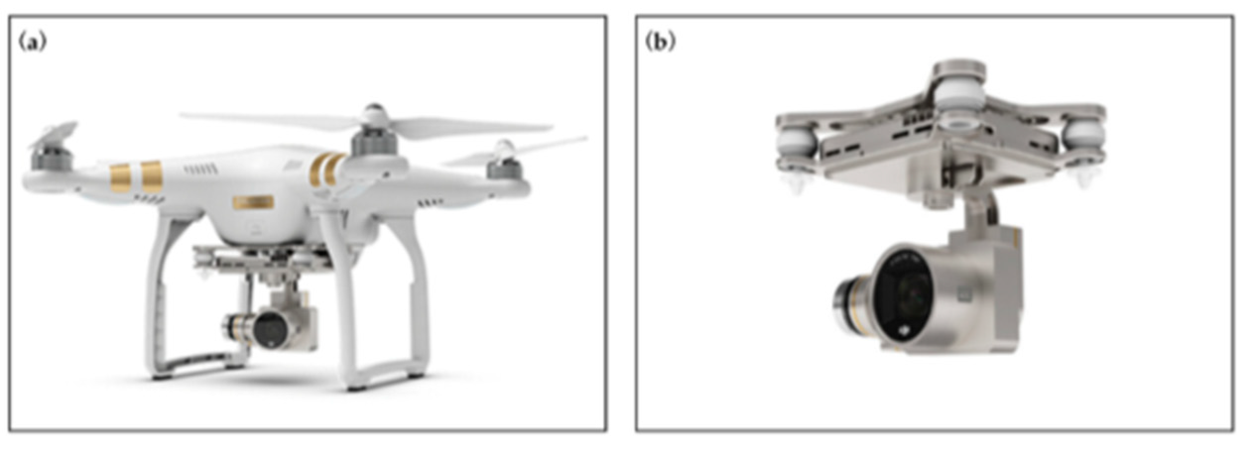
A multi-rotor UAV named Phantom 3 Professional (DJI-Innovations Inc., Shenzhen, China) was used to acquire high spatial-resolution images at the aforementioned four growth stages in this study (Figure 2). The UAV was equipped with a 12.4 megapixel visible light (RGB) built-in camera. A three-axis gimbal integrated with the inertial navigation system stabilized the camera during flight. The RGB aerial images were acquired with a resolution of 4000 × 3000 pixels (ground resolution: 1.66 cm) at a sensing height of 30 m and were saved with GPS location information in .raw format. The UAV images were collected under clear skies and low wind speed conditions between 10:30 a.m. and 1:30 p.m. of local time. The UAV aviated automatically based on the preset flight waypoints, leading to approximately 80% forward overlap and 60% side overlap controlled by the DJI GS Pro ground station application. The ISO of the camera was set as 100 and a fixed exposure was used according to the lighting conditions for each flight. Following the processing procedure of Lu et al. [20]; image alignment, georeferencing, mosaicking, dense point cloud construction, orthoimage generation, and calibration were conducted using PhotoScan Professional software (Agisoft LLC, ST. Petersburg, Russia) and ENVI/IDL software (Harris Geospatial Solutions, Inc., Broomfield, CO, USA) based on the GPS location and camera internal parameters from each aerial image.

2.3. Image Processing

2.3.1. Color Index (CI) Calculation

After all essential image processing, digital number (DN) values of R, G and B channels for each plot were extracted from each image using the region of interest (ROI) tool in ENVI/IDL. The DN values of RGB channels in remotely sensed RGB images can quantitatively reflect the radiance and reflectance characteristics in visible spectrum of crop canopy [26]. Normalized DNs (r, g and b, Equations (1)–(3)) were reported to have superior capacity for vegetation estimation compared to original RGB DN values [27]. As shown in Table 2, 12 types of CIs were selected and evaluated in this study.
r = R / ( R + G + B ) ,
g = G / ( R + G + B ) ,
b = B / ( R + G + B ) ,
where R, G, and B are the DNs of the red, green, and blue bands of the ROIs of each plot in the UAV-based images, respectively.

2.3.2. Texture Measurements

The grey level co-occurrence matrix (GLCM) [24]—one of the commonly used texture algorithms—was chosen to test the feasibility of using texture information from UAV-based RGB images for rice LAI estimation. A GLCM contains information about the positions of pixels that have similar grey level values, from which texture features representing the spatial arrangements of image colors or intensities can be computed. Eight GLCM-based textures, including mean (mea), variance (var), homogeneity (hom), contrast (con), dissimilarity (dis), entropy (ent), second moment (sem), and correlation (cor) were calculated using the ENVI/IDL software for each plot and each band of the digital images, respectively. Notably, entropy measures the disorder or randomness of color distribution and the second moment indicates textural uniformity of an image by measuring the angular relationship between neighboring pixels. The smallest window size (3 × 3 pixels) was used in the calculations of these textures. Moreover, in order to combine two different textures, the NDTI was calculated in this study based on Equation (4) [23]. Next, the calculated NDTIs were evaluated for rice LAI estimation and were further compared with traditional CIs.
NDTI   ( T 1 ,   T 2 ) = ( T 1 T 2 ) / ( T 1 + T 2 ) ,
where T 1 and T 2 represent two different randomly selected textures.

2.4. Regression Modeling Methods

2.4.1. Simple Linear Regression (LR)

Correlation analysis was conducted based on simple linear regression (LR) between rice LAI and each CI, texture, and NDTI, respectively. Due to their simple and understandable model structure, LR models have great applicability for practical use. The predictive performance of each single variable was also evaluated and compared based on LR models for rice LAI estimation. The LR models were built using the basic function shown in Equation (5).
LAI = b X + a ,
where LAI represents the rice leaf area index, X represents the single input predictor variable, b and a represent the slope and intercept of the fitted line of the LR model, respectively.

2.4.2. Multiple Linear Regression (MLR)

Different multivariate regression modeling methods, as introduced in Section 2.4.2, Section 2.4.3, Section 2.4.4 and Section 2.4.5, were used to test the potential of combining various color indices with textures for rice LAI estimation.
Multiple linear regression (MLR) is the most common form of linear regression which takes practical utilization of multivariate inputs. MLR has a relatively simple model form, shown as Equation (6), with great interpretability.
LAI = β 0 + β 1 X 1 + β 2 X 2 + β 3 X 3 + + β n X n ,
where X 1 ,   X 2 ,   , X n represent the input predictor variables of MLR, and β 0 ,   β 1 ,   β 2 ,   , X n represent the parameters of each variable, respectively.

2.4.3. Principal Component Regression (PCR) and Partial Least Squares Regression (PLS)

Input predictor variables for practical predictive modeling can be correlated and contain similar predictive information. The high correlation among each predictors would cause high variability and potential instability of the ordinary multiple linear regression [38]. Therefore, in order to reduce the dimension of the predictor space and improve the estimation performance of the model, this study adopted two solutions: (1) preprocessing based on principal component analysis (PCA); and (2) simultaneously conducting dimensionality reduction and regression by partial least squares.
Principal component regression (PCR) is a regression method that preprocesses predictors through PCA before performing regression [39]. The input predictor variables in PCA are converted into unrelated variable components through linear changes. Then, the transformed principal components are sorted according to the variability. The relationship between the predictor and response variables are characterized by the direction of the maximum variation. Finally, the regression models are built based on these PCA components, which contain most of the information of the input predictor variables. PCR is an unsupervised dimension reduction method and the tuning parameter that needs to be optimized is the number of principal components (PCR #Components).
PLS can convert several highly correlated predictors into a small number of uncorrelated variables, reducing the collinearities among them [40,41]. The PLS is originated with the nonlinear iterative partial least squares (NUPALS) algorithm provided by Herman Wold [41], which can be used to interactively determine the potential relationship between the highly correlated predictor variables and the response variable [38]. PLS takes both the response and predictor variables into consideration while balancing the predictive performance and dimensionality reduction in the process. Unlike the PCR method, PLS can be seen as a supervised dimension reduction method, and the components (PLS #Components) is a critical tuning parameter in its modeling.

2.4.4. Random Forest (RF)

Random Forest (RF) is a powerful machine learning algorithm, which has attracted wide attention. It is a nonlinear integrated modeling method based on multiple decision tree, and is composed of Breiman Leo’s autonomous resampling method (Bootstrap) [42] and the random subspace method introduced by Tin Kam Hom [43]. RF can be used for classification, regression, and clustering. It shows a promising capability to address the issue of overfitting as it can evaluate the importance of component predictor variables and can partly handle the multicollinearity among these variables while showing great tolerance to outliers and noises. Two tuning parameters are required in the RF process: the number of randomly selected predictors at each segmentation point (mtry) and the number of regression trees (ntree). Using a large number of regression trees to establish forests would not adversely affect the model’s predictive performance as introduced by Breiman et al. [42]. Therefore, the ntree was fixed at 1000 and only the mtry was adjusted to optimize the RF models in this study.

2.4.5. Support Vector Machine (SVM)

Support vector machine (SVM) proposed by Cortes and Vapnik [44] is a powerful machine learning method that can be used for pattern recognition and non-linear regression. The SVM regression was originally developed in the framework of a classification model, and its main idea was to establish a classification hyperplane as the decision boundary to maximize the distance between the decision boundary and the closest training point as well as to approximately minimize the structural risk [38]. SVM shows good potential for its versatility, robustness, and validity. A radial basis function (RBF) was selected in this study as the kernel function for SVM modeling. The tuning parameters of this SVM regression model are the scale parameter of RBF (σ) and the cost parameter (Cost). The cost parameter is the main tool for adjusting the complexity of the model, and it shows great flexibility compared to other parameters [38,45]. In this study, a fixed σ value for each specific type of input variables of each SVM models was automatically estimated based on the kernel-based machine learning method provided by the ksvm function in R package ‘kernlab’ [46]. Cost was further tuned to optimize the predictive performance of the SVM models.

2.5. Statistical Analysis

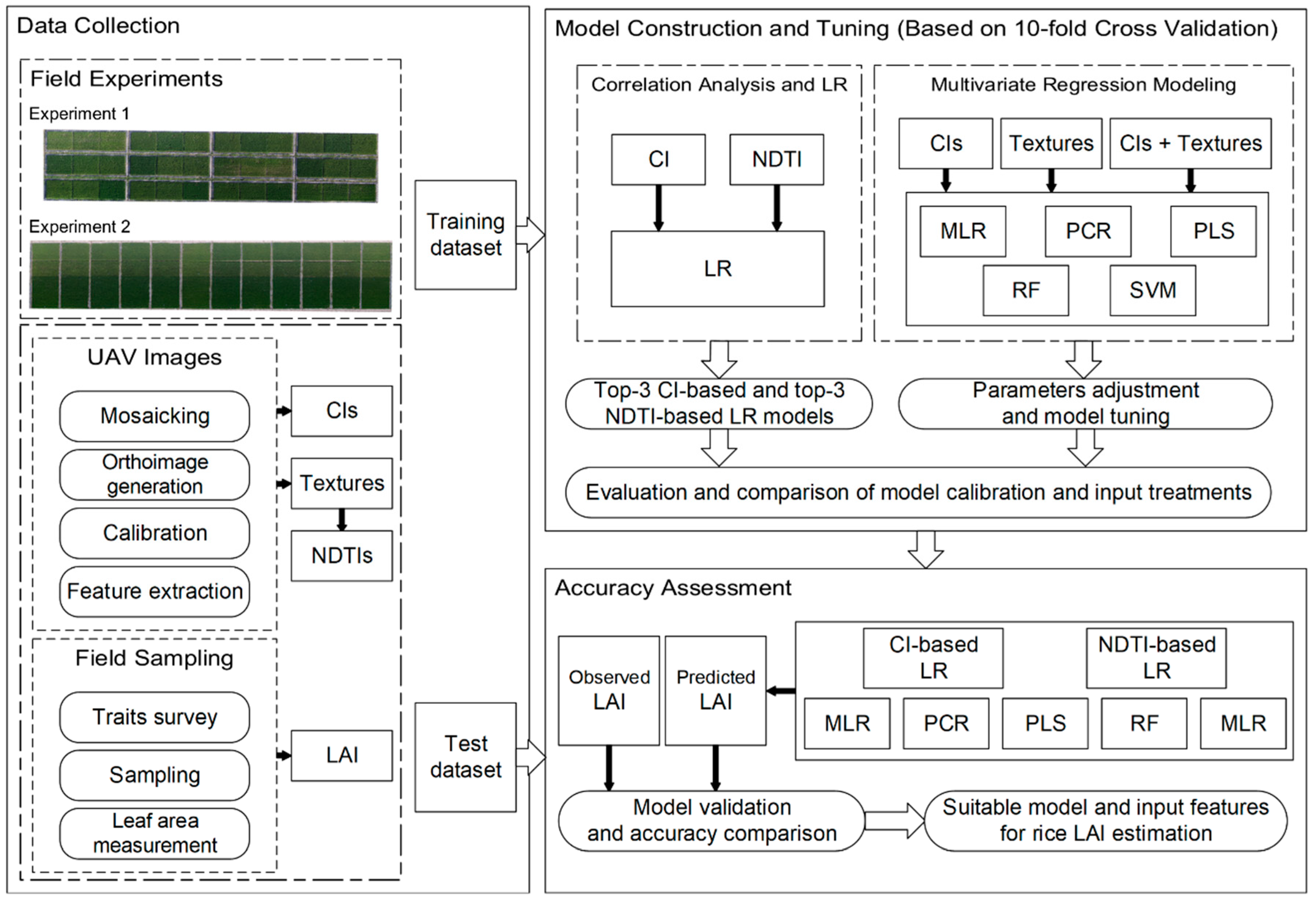
The procedure of statistical analysis after data collection is summarized by the flowchart in Figure 3. All the samples (n = 336) were pooled and randomly split into three parts to cover most characteristics of different experimental treatments and establish eurytopic models for rice LAI monitoring, and each split part covered all the possible treatments in Experiments 1 and 2. Two parts of the samples were selected as the training dataset (n = 224) while the remaining part was used as the test dataset (n = 112). Using a repeated resampling method of 10-fold cross-validation, the training set was used not only to tune and estimate the models, but also to evaluate their initial predictive performance. Cross-validated coefficient of determination (R2, Equation (7)) and root mean square error (RMSE, Equation (8)) were calculated to indicate the training and resampling results. LR models were established using inputs of each selected CI and NDTI. The correlations between rice LAIs and each texture and texture index were also analyzed based on the performance of the LR models, respectively. MLR, PCR, PLS, RF, and SVM regression models were constructed and adjusted using the training set with inputs of all the CIs, all the textures, or the combined CIs and textures, respectively. The accuracies of these regression models were assessed using the test data samples by measuring the R2, RMSE, and MAE Equation (9) between the predicted LAIs and the observed LAIs. Both RMSE and MAE indicate the average prediction error. However, the RMSE is more sensitive to large errors due to its quadratic scoring rule, while the MAE measures the absolute differences between prediction and actual observation. All the statistical analysis was performed using R software (v. 3.4.4., R Development Core Team, 2018).
R 2 = 1 i = 1 n ( y i y ^ i ) 2 i = 1 n ( y i y ¯ i ) 2 ,
RMSE = 1 n i = 1 n ( y i y ^ i ) 2 ,
MAE = 1 n i = 1 n | y i y ^ i | ,
where y i and y ^ i are the observed and predicted values of LAI, respectively; n is the number of samples.

3. Results

3.1. Variability of Rice Leaf Area Index

The LAIs of rice varied greatly, as expected, in terms of nitrogen rate, crop variety, growth stage, site, treatment, and year (Table 3). An increasing trend of LAI was shown in both the training set and test set at the four growth stages covering most of the growing cycle of rice. The LAI values across the growth stages ranged from 0.25 to 10.35 in the training set and from 0.29 to 10.05 in the test set. Besides, the large LAI variability at and across different growth stages was supposed to cover most of the possible situations, which also made it conceivable to test the capacity of using the UAV remotely sensed data for rice LAI estimation.

3.2. Simple Linear Regression Modeling for LAI Estimation

Figure 4 shows the performance (estimated by R2 and RMSE) of the LAI predictive models based on each of the 12 CIs using 10-fold cross-validation. The VARI and IKAW presented strong LR accuracy with rice LAI at and across all four stages compared to other CIs. Most of the CI-based LR models for LAI estimation showed relatively higher R2 and lower RMSE at the tillering stage than those of the subsequent three growth stages. The VARI-based LR model exhibited the best predictability for rice LAI across all the growth stages (R2 = 0.74, RMSE = 1.13).
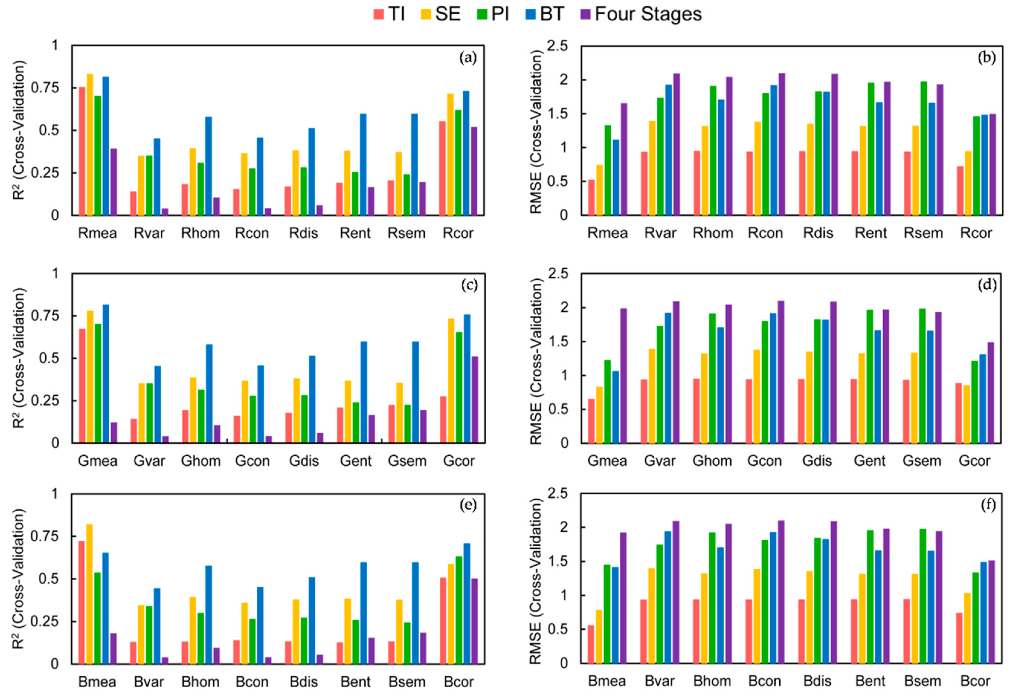
The linear relationships between rice LAI and the textures of R (Figure 5a,b), G (Figure 5c,d) and B (Figure 5e,f) channels varied greatly at different growth stages and textures. Most single textures showed poor predictive performance for LAI estimation across the growth stages except for the correlation (Rcor, Gcor, Bcor) and mean (Rmea, Gmea, Bmea) textures. As shown in Figure 5, similar cross-validated R2 and RMSE values were exhibited for the models based on the same textures of different color bands. This is because texture measurements highlight the spatial arrangement or relationship of pixel values in a neighborhood and similar spatial patterns appeared in the three color bands in this study. Across all the growth stages, the texture-based LR models for LAI estimation were not satisfactory with the best single texture of Rcor (R2 = 0.52, RMSE = 1.48). Therefore, it seems critical to combine different texture features for predictive purpose.
Utilization of NDTI is one of the promising solutions of combining two different textures for LAI estimation. Figure 6 shows the cross-validated R2 of LR models based on the NDTI with randomly selected T1 and T2 at and across different growth stages. The R2 values of these models varied notably among four growth stages. Unlike the CI-based ones, most NDTI-based LR models performed better during the booting stage (Figure 6d) as compared to other three stages. However, most NDTIs showed poor associations with rice LAI across all four growth stages except for NDTI (Rmea, Bmea), NDTI (Rmea, Gmea) and NDTI (Rcor, Bcor) (Figure 6e), indicating the importance of texture selection when using NDTI-based models for different stages.
Table 4 lists the top CI-based and NDTI-based LR models sorted by the cross-validated R2 and RMSE. VARI ranked the first (R2 = 0.74, RMSE = 1.13) among CIs followed by IKAW (R2 = 0.71, RMSE = 1.16) and NGRDI (R2 = 0.68, RMSE = 1.24) whereas NDTI (Rmea, Gmea) (R2 = 0.72, RMSE = 1.15), NDTI (Rmea, Bmea) (R2 = 0.71, RMSE = 1.17), and NDTI (Rcor, Bcor) (R2 = 0.58, RMSE = 1.38) were the top three NDTI-based training models. Therefore, these six LR models were chosen as the representative LR models and their accuracies were further evaluated using individual test dataset in Section 3.4.

3.3. Multivariate Regression Modeling

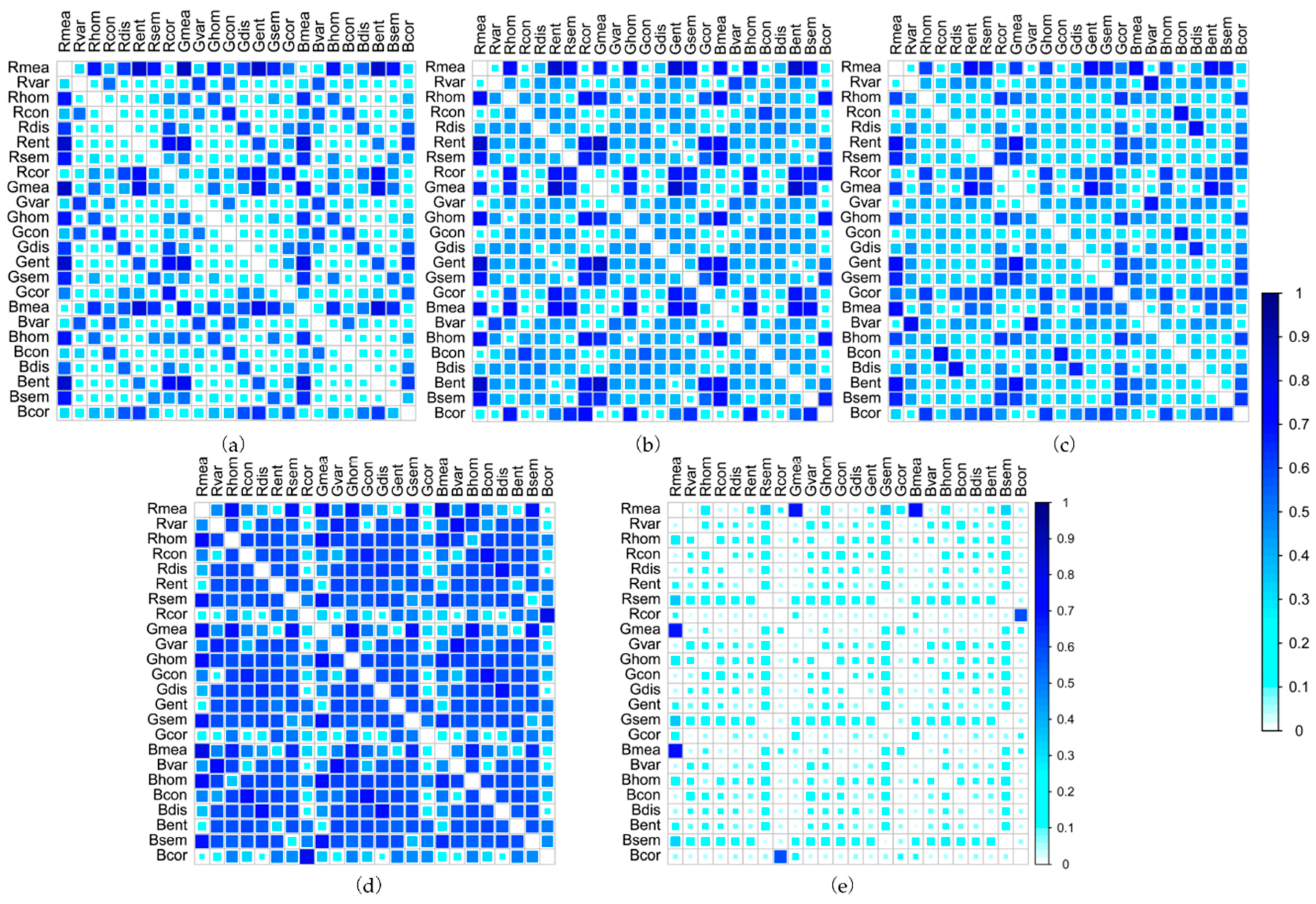
Without feature selection or data dimension reduction, the MLR models exhibited the cross-validated RMSE values of 0.92, 0.99, and 0.86 for the three input sets (CIs, textures, and Cis + Textures), respectively. However, some of the predictors within CIs or textures are highly correlated (Figure 7), indicating the potential issue of overfitting by simply using all the CIs or textures together for MLR modeling.
Figure 8 demonstrates the tuning process of PCR and PLS models with the three input sets, respectively. When the number of PCR and PLS components increased, the cross-validated RMSE decreased sharply first and then remained relatively stable. Using all the CIs as input variables, the PLS model achieved a minimum RMSE of 0.91 with six components, while the PCR attained the same minimum RMSE with seven components. Using all the textures as inputs, both the PCR and PLS obtained the same minimum RMSE (0.96) with 15 components. When combining all the CIs and textures as inputs, a minimum RMSE (0.84) was achieved by the PLS model with 25 components and PCR model with 23 components, respectively.
With a fixed tree number of 1000, RF models were trained and tuned by adjusting the mtry value, the number of randomly selected predictors (Figure 9). For the RF models using all the CIs as inputs, the cross-validated RMSE varied a lot, with the minimum value (0.97) achieved when mtry was set to 4. In contrast, for the texture-based RF models, the RMSE decreased steadily when the mtry value was increased from 2 to around 15, and then remained roughly stable. The minimum RMSE (0.93) was achieved when mtry was set to 21. The RF models based on the combined inputs of CIs and textures reached a minimum RMSE (0.90) when mtry value was 7.
The SVM regression modeling in this study was conducted using the kernel function of RBF. After automatically estimating the parameter σ of RBF, the cost parameter Cost was tuned for each SVM model to find the minimum RMSE. A similar concave upward trend was shown in all three cases: the cross-validated RMSE decreased first to reach the minimum value and then increased steadily when using a larger Cost (Figure 10). For the CI-based SVM models, the minimum RMSE (1.06) was reached when σ = 0.4511 and Cost = 8 (Figure 10a), while for the texture-based SVM model, the minimum RMSE (0.92) occurred when σ = 0.2146 and Cost = 8 (Figure 10b). For the case of using combined CI and texture inputs, the minimum RMSE (0.89) presented when σ = 0.7941 and Cost = 4 (Figure 10c).
The training results of different multivariate regression modeling methods are summarized in Table 5, which demonstrated that combining the CIs and textures provided better predictive models than using CIs or textures alone. Comparatively, the two improved multivariate linear regression methods PCR and PLS provided slightly better performance (cross-validated R2 = 0.86 and RMSE = 0.84).

3.4. Accuracy Assessment of the Predicted LAIs

Table 6 shows the predictive accuracy of the top-three CI-based and top-three NDTI-based LR models. Compared to other CIs, the VARI-based model showed the best performance with the least errors (R2 = 0.70, RMSE = 1.14, and MAE = 0.94) between the predicted and observed LAIs in the test dataset. The NDTI (Rmea, Gmea) based model had higher value of R2 (0.65) and smaller values of RMSE (1.23), and MAE (0.98) than the models based on other NDTIs. In general, the CI-based LR models performed slightly better than the NDTI-based ones.
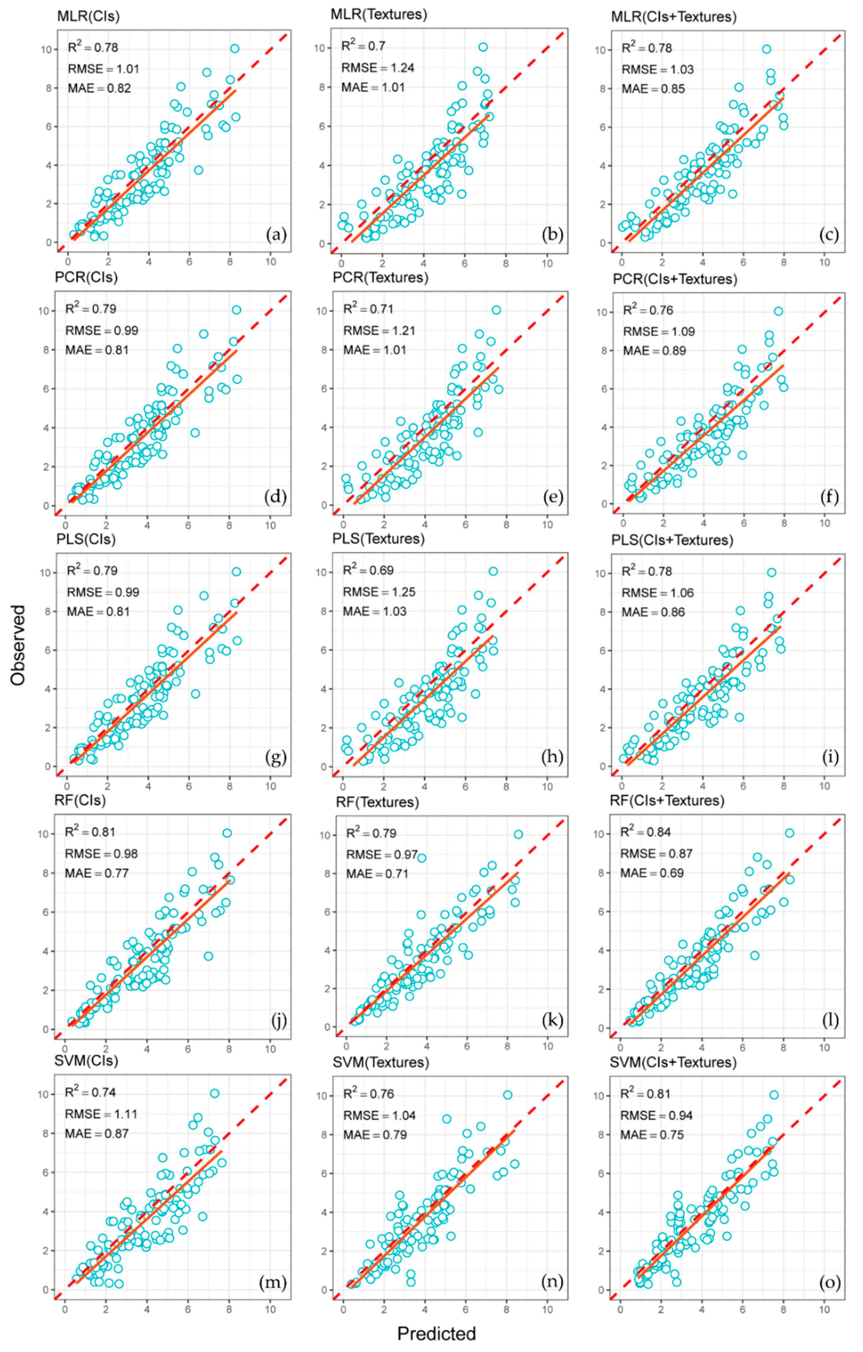
The scatter diagrams in Figure 11 reveal the accuracy assessment results of the multivariate regression models for cross-stage LAI estimation based on the independent test dataset. Overall, the predicted LAIs by all five multivariate methods showed moderately high accuracies when compared to the observed LAIs, with RMSE varying from 0.87 to 1.25 and MAE ranging from 0.69 to 1.03. As shown in Figure 11a–i, for the three linear regression methods (MLR, PCR, and PLS), the texture or CIs + Textures based models did not show better results than the ones only using CIs as inputs. Conversely, the RF and SVM models based on Cis + Textures performed better than the ones using CIs or textures only (Figure 11j–o).
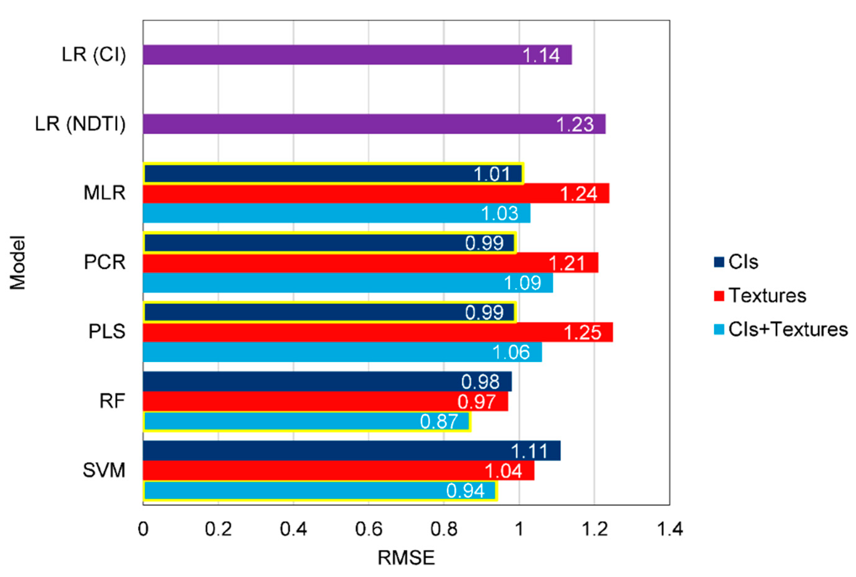
The RMSE values of the single LR and multivariate regression models were further evaluated and compared in Figure 12. The multivariate linear regression models with more inputs demonstrated better capability for practical LAI estimation than the single variable based LR models. In particular, the RF models had the lowest RMSEs or highest accuracies in all treatments of input variables (CIs-based RF: R2 = 0.81, RMSE = 0.98, and MAE = 0.77; textures-based RF: R2 = 0.79, RMSE = 0.97, and MAE = 0.71; CIs + Textures based RF: R2 = 0.84, RMSE = 0.87 and, MAE = 0.69). Therefore, the RF based on both color indices and textures was proven to be the optimal predictive method for rice LAI estimation using UAV-based digital imagery in this study.

4. Discussion

4.1. Combination of Color and Texture Information for Crop LAI Estimation

To test the applicability of using UAV imagery for LAI monitoring, 12 commonly used CIs were selected to build LR models. The results showed that visible atmospherically resistant index (VARI) had the best performance compared to other CIs in both training (R2 = 0.74) and test datasets (RMSE = 1.14, MAE = 0.94). Calculated from DN values of all three color channels (R, G, and B), the VARI has demonstrated excellent feasibility for crop biomass estimation [47] and yield prediction [48] in previous studies. VARI-based LR model has a simple and explicable structure, which is convenient for technical implementation and practical application.
Texture as a key spatial feature can be derived from UAV-based images and contains the canopy surface information for crop phenotypic research [24,49]. The normalized difference texture index (NDTI) proposed by Zheng et al. [23] follows the same structure of NDVI, but using two randomly selected GLCM-based textures instead. Their study demonstrated that the NDTI based on the mean textures of images in 800 and 550 nm wavebands from UAV-based multispectral imagery was superior to other VIs and NDTIs for estimating winter wheat aboveground biomass. NDTIs in this study were calculated with randomly selected GLCM-based textures from UAV-based RGB images. NDTI (Rmea, Gmea), NDTI (Rmea, Bmea), and NDTI (Rcor, Bcor) were the top-three NDTIs which showed great capability to estimate rice LAI with LR models. Textures represent spatial arrangements of image colors or intensities—rather than image pixel values. However, plant LAI is more directly associated with color information rather than the spatial arrangements of colors, even though texture features may add extra information for LAI estimation. In addition, the VARI makes use of color indices from three visible bands, whereas the NDTI only uses two textures. Therefore, this may leads to the better performance of the VARI compared to the NDTI.
Various multivariate regression modeling methods are promising for UAV-based applications in precision agriculture. Improved estimation of wheat biomass based on UAV sensing and RF modeling has been previously reported [20]. MLR has also been used to combine VIs and textures from UAV-based multispectral images for rice biomass monitoring in order to provide better prediction [23]. In this study, the RF model coupled with CIs and textures showed better estimation performance than traditional CI-based models.

4.2. Comparison of Different Multivariate Regression Methods

Compared to traditional MLR model, PCR and PLS represent two modified multiple linear regression methods that implement supervised and unsupervised process to reduce dimensions of input variables, respectively [38]. The superiority of dimension reduction was partly shown by the improved training performance of PCR and PLS (larger R2 values and smaller RMSEs than MLR) in Table 5. Through the pre-processing of PCA, PCR converts the input variables into several unrelated variable components, which cover the variability present throughout the predictor space. Unlike PCR, PLS reduces the dimension while maintaining the relationship between LAI and variable components. By reducing the complexity of the predictor space and model structure, PCR and PLS led to a relatively better cross-validated training result than traditional MLR.
However, MLR, PLS, and PCR showed some performance deterioration in Figure 11 when comparing the accuracy assessment results with the cross-validated training outcomes (Table 5). This performance deterioration could be attributed to the fact that the predictor components might not have a causal relationship with rice LAI, and despite the dimension reduction processes of PCR and PLS, multicollinearity might still exist in the CIs and textures (Figure 7)—leading to overfitting and poor predictive ability of these models. Therefore, pre-selection of input variables based on pre-analysis of the correlations among input predictors and utilization of indicators such as variance inflation factor (VIF) have been suggested to resolve the aforementioned issue in future studies [50,51]. However, the existence of nonlinear relationships between LAI and the input predictors (CI or texture) cannot be overlooked, which is difficult to estimate by linear regression-based models. This indicates the potential applicability of some other predictive modeling methods with nonlinear structures.
RF and SVM are two powerful predictive modeling techniques that can theoretically solve the issue of multicollinearity of the predictor variables. However, in this study, the CI-based SVM model did not exhibit better predictive performance than other modeling methods including RF (Figure 12). This may be caused by the defective parameter setting of Cost and σ. Considering the 12 CIs used for SVM modeling, the large number of Cost (8) may lead to a complex model structure and the potential risk of overfitting and poor predictive ability [44]. This issue needs to be further analyzed by considering factors such as detailed model structure, kernel function selection, and superior approaches for parameter setting.
With the smallest RMSE values, RF models achieved the best predictive results in all input treatments (Figure 12). In fact, contrary to the accuracy assessment results, the RF model did not show superior performance in the training process as compared to PLS and PCR models. Breiman [42] showed that RF can improve error rates by selecting many powerful, independent, and complex learners who exhibit low bias in the process of variance reduction. Since each learner is independent from all other learners, RF can be more robust to noises contained in the response variables and may overcome overfitting—resulting in exceptional predictive performance.

4.3. Potential of Consumer-Grade UAV-Based Digital Imagery for Crop Monitoring

Previous research has revealed significant differences in the results of UAV RS-based crop growth monitoring due to the use of different sensors [14]. With the exception of a few studies using Lidar [52] and non-imaging active or passive canopy sensors [7,53], most of the UAV-based studies have used imaging spectrometers or multispectral [16,48] and hyperspectral cameras [19]. However, professional imaging sensors, UAV systems, and their supporting software may lead to a high total cost for ordinary consumers and cause challenges for technical promotion.
On the contrary, consumer-grade UAVs and their built-in digital cameras offer obvious advantages of low cost (totally US $1200 for hardware cost in this study) and multiple uses. Besides, the large consumer-grade UAV market has not only attracted plentiful agricultural studies, but also accelerated the integration of more cutting-edge artificial intelligence (AI) and the internet of things (IoT) technologies into applications [54]. The rapid development of hardware and software for consumer-level UAVs has partly reshaped the industry of UAV-based precision agriculture, lowering application barriers and promoting technical expansion. For example, more mobile applications, such as Skippy Scout (DroneAg, Alnwick, UK), can provide integrated and automated solutions of UAV flight planning, operating, imagery capturing, and data analysis for crop scouting [55]. Therefore, A consumer-grade UAV with a digital camera can serve as a cheap and easy-to-use UAV RS solution for crop growth monitoring and precision agriculture [20,56].
Considering remotely sensed variables, traditional spectral indices such as VIs or CIs have been widely used in UAV RS-based crop biomass estimation [57], flower count [58], vegetation detection [59], yield prediction [19,48], and other applications of precision agriculture [60]. On the other hand, other studies have also used spatial information derived from UAV-based imagery, such as digital crop surface models (CSMs) [36], degree of canopy cover [61], plant height [36], and textures [49] for crop growth monitoring. It has been noted that the digital images collected by consumer-grade UAVs can take advantages of both sides to provide spectral and spatial information such as CIs [20], CSMs [62] and textures [49]. Moreover, proper multivariate regression methods can also improve the utilization of various UAV image-derived variables, as demonstrated by this and previous studies [20,63].
Apart from aforementioned advantages of consumer-grade UAV sensing, some further considerations regarding the practical use of this system are necessary. The first issue is the impact caused by the ground or spatial resolution of the UAV imagery. The canopy information contained in a single pixel could vary significantly at different ground resolution settings. In this study, an ultra-high ground resolution of 1.66 cm was used for image capture and texture calculations. This resolution setting comes from the consideration that high spatial-resolution images contain more pure pixels of crop leaves, crop shadows and background than low-resolution images [64]. Yue et al. [49] evaluated the impact of UAV image’s ground resolution (1-, 2-, 5-, 10-, 15-, 20-, 25-, 30-cm) on GLCM-based textures and their capabilities for wheat biomass estimation. They found that textures derived from 1 cm ground resolution images were highly related to biomass, because the high-frequency information in most pure pixels of ultra-high-resolution images represents the scale of flourishing crops. Image ground resolution determines the contents in mixed pixels, which are further influenced by the canopy size and background information such as row spacing. Therefore, future studies are still needed to analyze the performance of textures at various ground resolutions, different stages with varying crop canopy sizes, and different background conditions controlled by farming operations.
In addition, the modeling methods and the extracted features still need to be improved. Although outstanding performance was achieved by combining CIs with textures in the RF model, the importance of each input variable for LAI estimation is still unclear. More promising modeling methods such as Bayesian linear regression [18], mixed-effect model [65,66], or deep learning [67] need to be tested with the most critical predictor features. Besides, the crop growth process is usually affected by various environmental factors such as temperature or sunshine duration. Accordingly, the spectral and texture features of the crop may vary nonlinearly with the growth process and growing environment. Therefore, it is important not only to summarize ideal indices consisting of sensitive spectral and texture features based on their underlying mechanism, but also to incorporate environmental variables from multiple times during the crop phenological cycle in the predictive models, in order to provide powerful and suitable models for practical uses.

5. Conclusions

This study showed the feasibility of using color indices and textures derived from images collected by a consumer-grade UAV to estimate rice LAI based on field measurements and comprehensive predictive modeling approaches. VARI and NDTI (Rmea, Gmea) showed the best performance in CI-based and NDTI-based LR models, respectively. Multivariate regression modeling methods (MLR, PLS, PCR, RF, and SVM) were further evaluated and compared using different input variable sets. RF showed the best ability to combine CIs and textures for rice LAI estimation (R2 = 0.84, RMSE = 0.87, and MAE = 0.69). Future investigations are necessary to consider the effects of UAV image resolution, feature extraction methods, and the underlying mechanisms of textures. Additionally, automated workflow for image acquisition, feature extraction, and better LAI estimation strategy is yet to be developed for practical uses of this sensing mode in the future.

Author Contributions

Q.C., Y.T., Y.Z. and W.C. conceived and designed the experiments; S.L. and Q.C. performed the experiments; S.L. and Q.C. analyzed the data and wrote the original manuscript; F.Y., S.T.A.-U.-K., H.Z., T.C., X.L., Y.T., Y.Z., and W.C. reviewed and revised the manuscript. All authors read and approved the final manuscript.

Funding

This research was funded by the National Key Research and Development Program (2016YFD0300608), the Fundamental Research Funds for the Central University (KYZ201502, KJQN201725), the National Natural Science Foundation of China (31601222, 31725020), the Natural Science Foundation of Jiangsu Province (BK20150663), the earmarked fund for Jiangsu Agricultural Industry Technology System (JATS [2018]290), the Priority Academic Program Development of Jiangsu Higher Education Institutions (PAPD) and the 111 project (B16026).

Acknowledgments

We would like to thank Ke Zhang, Zeyu Zhang, Jun He, Zhonghua Li, Qianliang Kuang, Xinzhong Ding and Jiameng Ni from the College of Agriculture, Nanjing Agricultural University (NAU), for their fieldwork and contributions in data collection. We would also like to thank Russell Yost from the Department of Tropical Plant and Soil Science in University of Hawai’i at Manoa for their contributions in reviewing and revising the manuscript.

Conflicts of Interest

The authors declare no conflict of interest.

References

  1. Watson, D.J. Comparative Physiological Studies on the Growth of Field Crops: II. The Effect of Varying Nutrient Supply on Net Assimilation Rate and Leaf Area. Ann. Bot. 1947, 11, 375–407. [Google Scholar] [CrossRef]
  2. Wells, R. Soybean Growth Response to Plant Density: Relationships among Canopy Photosynthesis, Leaf Area, and Light Interception. Crop Sci. 1991, 31, 755–761. [Google Scholar] [CrossRef]
  3. Loomis, R.S.; Williams, W.A. Maximum Crop Productivity: An Extimate 1. Crop Sci. 1963, 3, 67–72. [Google Scholar] [CrossRef]
  4. Richards, R.A.; Townley-Smith, T.F. Variation in leaf area development and its effect on water use, yield and harvest index of droughted wheat. Aust. J. Agric. Res. 1987, 38, 983–992. [Google Scholar] [CrossRef]
  5. Duchemin, B.; Maisongrande, P.; Boulet, G.; Benhadj, I. A simple algorithm for yield estimates: Evaluation for semi-arid irrigated winter wheat monitored with green leaf area index. Environ. Model. Softw. 2008, 23, 876–892. [Google Scholar] [CrossRef] [Green Version]
  6. Jefferies, R.A.; Mackerron, D.K.L. Responses of potato genotypes to drought. II. Leaf area index, growth and yield. Ann. Appl. Biol. 2010, 122, 105–112. [Google Scholar] [CrossRef]
  7. Li, S.; Ding, X.; Kuang, Q.; Ata-Ul-Karim, S.T.; Cheng, T.; Liu, X.; Tan, Y.; Zhu, Y.; Cao, W.; Cao, Q. Potential of UAV-Based Active Sensing for Monitoring Rice Leaf Nitrogen Status. Front. Plant Sci. 2018, 9, 1834. [Google Scholar] [CrossRef] [PubMed] [Green Version]
  8. Yao, Y.; Liu, Q.; Liu, Q.; Li, X. LAI retrieval and uncertainty evaluations for typical row-planted crops at different growth stages. Remote Sens. Environ. 2008, 112, 94–106. [Google Scholar] [CrossRef]
  9. Li, X.; Zhang, Y.; Luo, J.; Jin, X.; Xu, Y.; Yang, W. Quantification winter wheat LAI with HJ-1CCD image features over multiple growing seasons. Int. J. Appl. Earth Obs. Geoinf. 2016, 44, 104–112. [Google Scholar] [CrossRef]
  10. Dong, T.; Liu, J.; Shang, J.; Qian, B.; Ma, B.; Kovacs, J.M.; Walters, D.; Jiao, X.; Geng, X.; Shi, Y. Assessment of red-edge vegetation indices for crop leaf area index estimation. Remote Sens. Environ. 2019, 222, 133–143. [Google Scholar] [CrossRef]
  11. Liang, L.; Di, L.; Zhang, L.; Deng, M.; Qin, Z.; Zhao, S.; Lin, H. Estimation of crop LAI using hyperspectral vegetation indices and a hybrid inversion method. Remote Sens. Environ. 2015, 165, 123–134. [Google Scholar] [CrossRef]
  12. Zhang, J.; Liu, X.; Liang, Y.; Cao, Q.; Tian, Y.; Zhu, Y.; Cao, W.; Liu, X. Using a Portable Active Sensor to Monitor Growth Parameters and Predict Grain Yield of Winter Wheat. Sensors 2019, 19, 1108. [Google Scholar] [CrossRef] [PubMed]
  13. Zhang, K.; Ge, X.; Shen, P.; Li, W.; Liu, X.; Cao, Q.; Zhu, Y.; Cao, W.; Tian, Y. Predicting Rice Grain Yield Based on Dynamic Changes in Vegetation Indexes during Early to Mid-Growth Stages. Remote Sens. 2019, 11, 387. [Google Scholar] [CrossRef]
  14. Yang, G.; Liu, J.; Zhao, C.; Li, Z.; Huang, Y.; Yu, H.; Xu, B.; Yang, X.; Zhu, D.; Zhang, X.; et al. Unmanned Aerial Vehicle Remote Sensing for Field-Based Crop Phenotyping: Current Status and Perspectives. Front. Plant Sci. 2017, 8, 1111. [Google Scholar] [CrossRef] [PubMed]
  15. Colomina, I.; Molina, P. Unmanned aerial systems for photogrammetry and remote sensing: A review. ISPRS J. Photogramm. Remote Sens. 2014, 92, 79–97. [Google Scholar] [CrossRef] [Green Version]
  16. Yao, X.; Wang, N.; Liu, Y.; Cheng, T.; Tian, Y.; Chen, Q.; Zhu, Y. Estimation of Wheat LAI at Middle to High Levels Using Unmanned Aerial Vehicle Narrowband Multispectral Imagery. Remote Sens. 2017, 9, 1304. [Google Scholar] [CrossRef]
  17. Yue, J.; Feng, H.; Jin, X.; Yuan, H.; Li, Z.; Zhou, C.; Yang, G.; Tian, Q.; Yue, J.; Feng, H.; et al. A Comparison of Crop Parameters Estimation Using Images from UAV-Mounted Snapshot Hyperspectral Sensor and High-Definition Digital Camera. Remote Sens. 2018, 10, 1138. [Google Scholar] [CrossRef]
  18. Xu, X.Q.; Lu, J.S.; Zhang, N.; Yang, T.C.; He, J.Y.; Yao, X.; Cheng, T.; Zhu, Y.; Cao, W.X.; Tian, Y.C. Inversion of rice canopy chlorophyll content and leaf area index based on coupling of radiative transfer and Bayesian network models. ISPRS J. Photogramm. Remote Sens. 2019, 150, 185–196. [Google Scholar] [CrossRef]
  19. Kanning, M.; Kühling, I.; Trautz, D.; Jarmer, T. High-Resolution UAV-Based Hyperspectral Imagery for LAI and Chlorophyll Estimations from Wheat for Yield Prediction. Remote Sens. 2018, 10, 2000. [Google Scholar] [CrossRef]
  20. Lu, N.; Zhou, J.; Han, Z.; Li, D.; Cao, Q.; Yao, X.; Tian, Y.; Zhu, Y.; Cao, W.; Cheng, T. Improved estimation of aboveground biomass in wheat from RGB imagery and point cloud data acquired with a low-cost unmanned aerial vehicle system. Plant Methods 2019, 15, 17. [Google Scholar] [CrossRef] [Green Version]
  21. Li, W.; Niu, Z.; Chen, H.; Li, D.; Wu, M.; Zhao, W. Remote estimation of canopy height and aboveground biomass of maize using high-resolution stereo images from a low-cost unmanned aerial vehicle system. Ecol. Indic. 2016, 67, 637–648. [Google Scholar] [CrossRef]
  22. Li, S.; Liu, X.; Tian, Y.; Zhu, Y.; Cao, Q. Comparison RGB Digital Camera with Active Canopy Sensor Based on UAV for Rice Nitrogen Status Monitoring. In Proceedings of the 2018 7th International Conference on Agro-Geoinformatics (Agro-Geoinformatics), Hangzhou, China, 6–9 August 2018. [Google Scholar]
  23. Zheng, H.; Cheng, T.; Zhou, M.; Li, D.; Yao, X.; Tian, Y.; Cao, W.; Zhu, Y. Improved estimation of rice aboveground biomass combining textural and spectral analysis of UAV imagery. Precis. Agric. 2019, 20, 611–629. [Google Scholar] [CrossRef]
  24. Haralick, R.M.; Shanmugam, K.; Dinstein, I. Textural Features for Image Classification. IEEE Trans. Syst. Man Cybern. 1973, SMC-3, 610–621. [Google Scholar] [CrossRef] [Green Version]
  25. Sarker, L.R.; Nichol, J.E. Improved forest biomass estimates using ALOS AVNIR-2 texture indices. Remote Sens. Environ. 2011, 115, 968–977. [Google Scholar] [CrossRef]
  26. Hong, G.; Luo, M.R.; Rhodes, P.A. A study of digital camera colorimetric characterization based on polynomial modeling. Color Res. Appl. 2001, 26, 76–84. [Google Scholar] [CrossRef]
  27. Richardson, M.D.; Karcher, D.E.; Purcell, L.C. Quantifying turfgrass cover using digital image analysis. Crop Sci. 2001, 41, 1884–1888. [Google Scholar] [CrossRef]
  28. Gitelson, A.A.; Kaufman, Y.J.; Stark, R.; Rundquist, D. Novel algorithms for remote estimation of vegetation fraction. Remote Sens. Environ. 2002, 80, 76–87. [Google Scholar] [CrossRef] [Green Version]
  29. Woebbecke, D.M.; Meyer, G.E.; Von Bargen, K.; Mortensen, D.A. Color Indices for Weed Identification Under Various Soil, Residue, and Lighting Conditions. Trans. ASAE 1995, 38, 259–269. [Google Scholar] [CrossRef]
  30. Meyer, G.E.; Neto, J.C. Verification of color vegetation indices for automated crop imaging applications. Comput. Electron. Agric. 2008, 63, 282–293. [Google Scholar] [CrossRef]
  31. Mao, W.; Wang, Y.; Wang, Y. Real-time detection of between-row weeds using machine vision. In Proceedings of the 2003 ASAE Annual Meeting; American Society of Agricultural and Biological Engineers, Las Vegas, NV, USA, 27–30 July 2003. [Google Scholar]
  32. Neto, J.C. A combined statistical-soft computing approach for classification and mapping weed species in minimum -tillage systems. Ph.D. Thesis, University of Nebraska – Lincoln, Lincoln, NE, USA, August 2004. [Google Scholar]
  33. Tucker, C.J. Red and photographic infrared linear combinations for monitoring vegetation. Remote Sens. Environ. 1979, 8, 127–150. [Google Scholar] [CrossRef] [Green Version]
  34. Kawashima, S.; Nakatani, M. An algorithm for estimating chlorophyll content in leaves using a video camera. Ann. Bot. 1998, 81, 49–54. [Google Scholar] [CrossRef]
  35. Louhaichi, M.; Borman, M.M.; Johnson, D.E. Spatially located platform and aerial photography for documentation of grazing impacts on wheat. Geocarto Int. 2001, 16, 65–70. [Google Scholar] [CrossRef]
  36. Bendig, J.; Yu, K.; Aasen, H.; Bolten, A.; Bennertz, S.; Broscheit, J.; Gnyp, M.L.; Bareth, G. Combining UAV-based plant height from crop surface models, visible, and near infrared vegetation indices for biomass monitoring in barley. Int. J. Appl. Earth Obs. Geoinf. 2015, 39, 79–87. [Google Scholar] [CrossRef]
  37. Hague, T.; Tillett, N.D.; Wheeler, H. Automated crop and weed monitoring in widely spaced cereals. Precis. Agric. 2006, 7, 21–32. [Google Scholar] [CrossRef]
  38. Kuhn, M.; Johnson, K. Applied Predictive Modeling; Springer: New York, NY, USA, 2013; Volume 26. [Google Scholar]
  39. Massy, W.F. Principal components regression in exploratory statistical research. J. Am. Stat. Assoc. 1965, 60, 234–256. [Google Scholar] [CrossRef]
  40. Williams, P.; Norris, K. Near-Infrared Technology in the Agricultural and Food Industries; American Association of Cereal Chemists, Inc.: St. Paul, MN, USA, 1987. [Google Scholar]
  41. Wold, S.; Sjöström, M.; Eriksson, L. PLS-regression: A basic tool of chemometrics. Chemom. Intell. Lab. Syst. 2001, 58, 109–130. [Google Scholar] [CrossRef]
  42. Breiman, L. Random Forests. Mach. Learn. 2001, 45, 5–32. [Google Scholar] [CrossRef] [Green Version]
  43. Ho, T.K. The random subspace method for constructing decision forests. IEEE Trans. Pattern Anal. Mach. Intell. 1998, 20, 832–844. [Google Scholar] [CrossRef]
  44. Cortes, C.; Vapnik, V. Support-vector networks. Mach. Learn. 1995, 20, 273–297. [Google Scholar] [CrossRef]
  45. Caputo, B.; Sim, K.; Furesjo, F.; Smola, A. Appearance-based object recognition using SVMs: Which kernel should I use? In Proceedings of the NIPS Workshop on Statistical Methods for Computational Experiments in Visual Processing and Computer Vision, Whistler, BC, Canada, 13 December 2002. [Google Scholar]
  46. Karatzoglou, A.; Smola, A.; Hornik, K.; Zeileis, A. kernlab-an S4 package for kernel methods in R. J. Stat. Softw. 2004, 11, 1–20. [Google Scholar] [CrossRef]
  47. Kaivosoja, J.; Näsi, R.; Hakala, T.; Viljanen, N.; Honkavaara, E. Applying Different Remote Sensing Data to Determine Relative Biomass Estimations of Cereals for Precision Fertilization Task Generation. In Proceedings of the 8th International Conference on Information and Communication Technologies in Agriculture, Food and Environment (HAICTA 2017), Chania, Greece, 21–24 September 2017. [Google Scholar]
  48. Zhou, X.; Zheng, H.B.; Xu, X.Q.; He, J.Y.; Ge, X.K.; Yao, X.; Cheng, T.; Zhu, Y.; Cao, W.X.; Tian, Y.C. Predicting grain yield in rice using multi-temporal vegetation indices from UAV-based multispectral and digital imagery. ISPRS J. Photogramm. Remote Sens. 2017, 130, 246–255. [Google Scholar] [CrossRef]
  49. Yue, J.; Yang, G.; Tian, Q.; Feng, H.; Xu, K.; Zhou, C. Estimate of winter-wheat above-ground biomass based on UAV ultrahigh-ground-resolution image textures and vegetation indices. ISPRS J. Photogramm. Remote Sens. 2019, 150, 226–244. [Google Scholar] [CrossRef]
  50. Yue, J.; Feng, H.; Yang, G.; Li, Z. A Comparison of Regression Techniques for Estimation of Above-Ground Winter Wheat Biomass Using Near-Surface Spectroscopy. Remote Sens. 2018, 10, 66. [Google Scholar] [CrossRef]
  51. Myers, R.H. Classical and Modern Regression with Applications; Duxbury Press: Belmont, CA, USA, 1990. [Google Scholar]
  52. Li, W.; Niu, Z.; Wang, C.; Huang, W.; Chen, H.; Gao, S.; Li, D.; Muhammad, S. Combined use of airborne LiDAR and satellite GF-1 data to estimate leaf area index, height, and aboveground biomass of maize during peak growing season. IEEE J. Sel. Top. Appl. Earth Obs. Remote Sens. 2015, 8, 4489–4501. [Google Scholar] [CrossRef]
  53. Ni, J.; Yao, L.; Zhang, J.; Cao, W.; Zhu, Y.; Tai, X. Development of an Unmanned Aerial Vehicle-Borne Crop-Growth Monitoring System. Sensors 2017, 17, 502. [Google Scholar] [CrossRef] [PubMed]
  54. Snow, C. Seven Trends That Will Shape the Commercial Drone Industry in 2019. Available online: https://www.forbes.com/sites/colinsnow/2019/01/07/seven-trends-that-will-shape-the-commercial-drone-industry-in-2019/ (accessed on 31 May 2019).
  55. DroneAG Developing Skippy Scout App to Automate Drone Crop Scouting | Farm and Plant Blog. Available online: https://www.farmandplant.ie/blog/ag-equipment-news/2019/04/droneag-developing-skippy-scout-app-to-automate-drone-crop-scouting (accessed on 19 July 2019).
  56. Sanches, G.M.; Duft, D.G.; Kölln, O.T.; Luciano, A.C.D.S.; De Castro, S.G.Q.; Okuno, F.M.; Franco, H.C.J. The potential for RGB images obtained using unmanned aerial vehicle to assess and predict yield in sugarcane fields. Int. J. Remote Sens. 2018, 39, 5402–5414. [Google Scholar] [CrossRef]
  57. Han, L.; Yang, G.; Dai, H.; Xu, B.; Yang, H.; Feng, H.; Li, Z.; Yang, X. Modeling maize above-ground biomass based on machine learning approaches using UAV remote-sensing data. Plant Methods 2019, 15, 10. [Google Scholar] [CrossRef] [PubMed]
  58. Wan, L.; Li, Y.; Cen, H.; Zhu, J.; Yin, W.; Wu, W.; Zhu, H.; Sun, D.; Zhou, W.; He, Y. Combining UAV-Based Vegetation Indices and Image Classification to Estimate Flower Number in Oilseed Rape. Remote Sens. 2018, 10, 1484. [Google Scholar] [CrossRef]
  59. Torres-Sánchez, J.; López-Granados, F.; Peña, J.M. An automatic object-based method for optimal thresholding in UAV images: Application for vegetation detection in herbaceous crops. Comput. Electron. Agric. 2015, 114, 43–52. [Google Scholar] [CrossRef]
  60. Rasmussen, J.; Ntakos, G.; Nielsen, J.; Svensgaard, J.; Poulsen, R.N.; Christensen, S. Are vegetation indices derived from consumer-grade cameras mounted on UAVs sufficiently reliable for assessing experimental plots? Eur. J. Agron. 2016, 74, 75–92. [Google Scholar] [CrossRef]
  61. Duan, T.; Zheng, B.; Guo, W.; Ninomiya, S.; Guo, Y.; Chapman, S.C. Comparison of ground cover estimates from experiment plots in cotton, sorghum and sugarcane based on images and ortho-mosaics captured by UAV. Funct. Plant Biol. 2017, 44, 169–183. [Google Scholar] [CrossRef]
  62. Bendig, J.; Bolten, A.; Bennertz, S.; Broscheit, J.; Eichfuss, S.; Bareth, G. Estimating Biomass of Barley Using Crop Surface Models (CSMs) Derived from UAV-Based RGB Imaging. Remote Sens. 2014, 6, 10395–10412. [Google Scholar] [CrossRef] [Green Version]
  63. Yuan, H.; Yang, G.; Li, C.; Wang, Y.; Liu, J.; Yu, H.; Feng, H.; Xu, B.; Zhao, X.; Yang, X. Retrieving Soybean Leaf Area Index from Unmanned Aerial Vehicle Hyperspectral Remote Sensing: Analysis of RF, ANN, and SVM Regression Models. Remote Sens. 2017, 9, 309. [Google Scholar] [CrossRef]
  64. Wu, J.; Lee, D.; Jiao, L.; Shi, G. Laplacian pyramid-based downsampling combined with directionlet interpolation for low-bit rate compression. In Proceedings of the MIPPR 2009: Remote Sensing and GIS Data Processing and Other Applications; International Society for Optics and Photonics, Yichang, China, 30 October–1 November 2009. [Google Scholar]
  65. Wang, Y.; Zhang, K.; Tang, C.; Cao, Q.; Tian, Y.; Zhu, Y.; Cao, W.; Liu, X. Estimation of Rice Growth Parameters Based on Linear Mixed-Effect Model Using Multispectral Images from Fixed-Wing Unmanned Aerial Vehicles. Remote Sens. 2019, 11, 1371. [Google Scholar] [CrossRef]
  66. Zuur, A.F.; Ieno, E.N.; Walker, N.J.; Saveliev, A.A.; Smith, G.M. Mixed Effects Models and Extensions in Ecology with R; Springer: New York, NY, USA, 2009. [Google Scholar]
  67. Kuwata, K.; Shibasaki, R. Estimating crop yields with deep learning and remotely sensed data. In Proceedings of the 2015 IEEE International Geoscience and Remote Sensing Symposium (IGARSS), Milan, Italy, 26–31 July 2015. [Google Scholar]
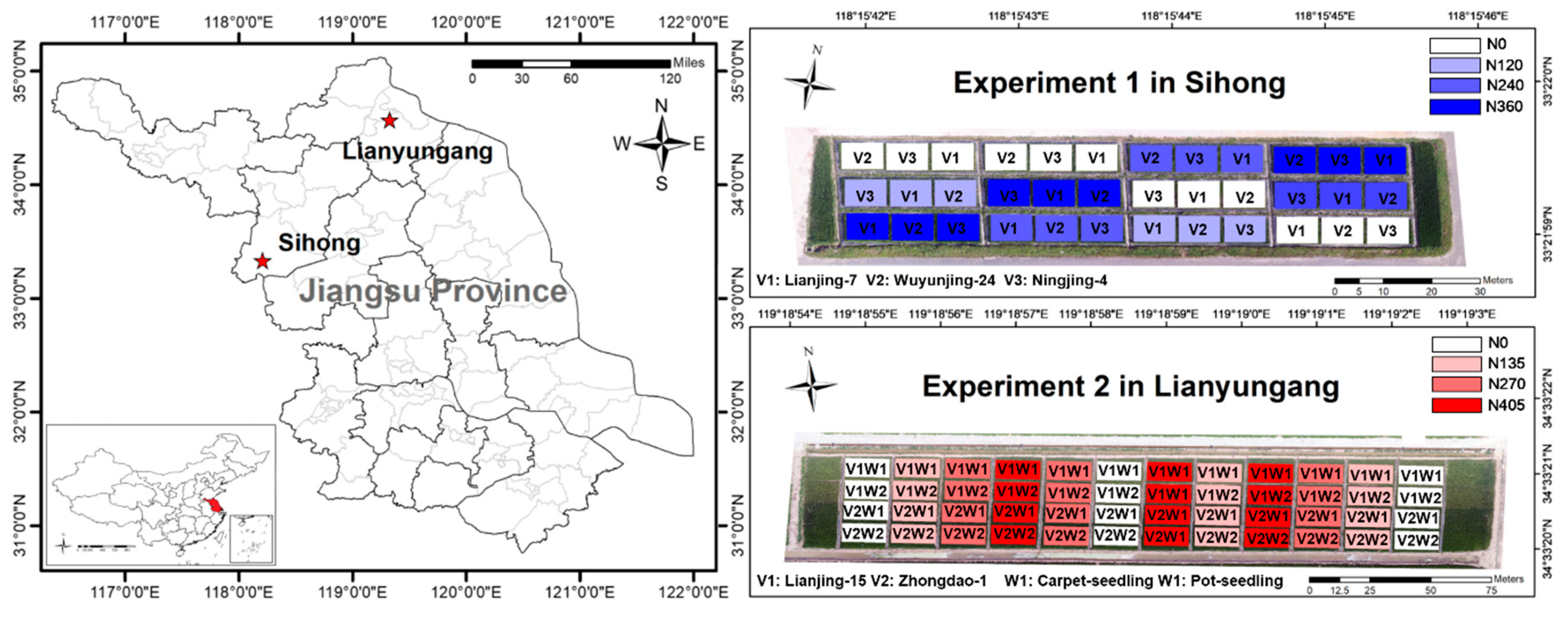
Figure 1. Locations and treatments of the experiments in this study.
Remotesensing 11 01763 g001
Figure 2. The unmanned aerial vehicle (a) and its built-in digital camera (b) used in this study.
Remotesensing 11 01763 g002
Figure 3. Experiment methodology and procedure of statistical analysis in this study.
Remotesensing 11 01763 g003
Figure 4. Cross-validated R2 (a) and RMSE (b) of the CI-based simple linear regression models for rice LAI estimation at and across the growth stages of tillering (TI), stem elongation (SE), panicle initiation (PI), and booting (BT), respectively.
Remotesensing 11 01763 g004
Figure 5. Cross-validated R2 (a,c,e) and RMSE (b,d,f) of the single texture-based simple linear regression models for rice LAI estimation at and across the growth stages of tillering (TI), stem elongation (SE), panicle initiation (PI), and booting (BT), respectively.
Remotesensing 11 01763 g005
Figure 6. Cross-validated R2 of the NDTI-based simple linear regression models for rice LAI estimation at the tillering (a), stem elongation (b), panicle initiation (c), booting (d), and across all four stages (e). The x-axis and y-axis represent the texture selections of T1 and T2 for NDTI calculation, respectively.
Remotesensing 11 01763 g006
Figure 7. Pearson’s correlation coefficient (r) between UAV RGB image-derived color indices and textures.
Remotesensing 11 01763 g007
Figure 8. Cross-validated RMSE values over the number of components for PCR and PLS using inputs of CIs (a), textures (b), and combined CIs and textures (c), respectively.
Remotesensing 11 01763 g008
Figure 9. Cross-validated RMSE values over different mtry values using inputs of CIs (a), textures (b), and combined CIs and textures (c), respectively (number of trees was set as 1000).
Remotesensing 11 01763 g009
Figure 10. Cross-validated RMSE values over the parameter Cost using inputs of CIs (a, σ = 0.4511), textures (b, σ = 0.2146), and combined CIs and textures (c, σ = 0.7941), respectively.
Remotesensing 11 01763 g010
Figure 11. Accuracy assessment results of the MLR (ac), PCR (df), PLS (gi), RF (jl), and SVM (mo) models for LAI estimation based on test datasets with inputs of CIs, textures, and CIs + Textures, respectively.
Remotesensing 11 01763 g011
Figure 12. Comparison of the predictive accuracies of the best CI-based LR, best NDTI-based LR, and multivariate regression models (MLR, PCR, PLS, RF, and SVM) in test datasets with inputs of CIs, Textures and combined CIs + Textures, respectively. The optimal input treatment (minimum RMSE) of each multivariate regression model is highlighted by yellow frame.
Remotesensing 11 01763 g012
Table 1. Description of samplings in this study.
ExperimentYearLocationSamplesTransplanting DateSensing and Sampling Date
Experiment 12016Sihong14425 June27 July (TI),
3 August (SE),
11 August (PI),
18 August (BT)
Experiment 22017Lianyungang19219 June27 July (TI),
3 August (SE),
10 August (PI),
20 August (BT)
TI: tillering; SE: stem elongation; PI: panicle initiation; and BT: booting.
Table 2. Summary of the spectral color indices (CIs) used in this study for LAI estimation.
CINameFormulaReference
VARIVisible Atmospherically Resistant Index(g − r)/(g + r − b)Gitelson et al. [28]
ExGExcess Green Vegetation Index2g − r − bWoebbecke et al. [29]
ExRExcess Red Vegetation Index1.4r − gMeyer et al. [30]
ExBExcess Blue Vegetation Index1.4b − gMao et al. [31]
ExGRExcess Green minus Excess Red Vegetation IndexE × G − E × RNeto et al. [32]
NGRDINormalized Green-Red Difference Index(g − r)/(g + r)Tucker [33]
MGRVIModified Green Red Vegetation Index(g2 − r2)/(g2 + r2)Tucker [33]
WIWoebbecke Index(g − b)/(r − g)Woebbecke et al. [29]
IKAWKawashima Index(r − b)/(r + b)Kawashima et al. [34]
GLAGreen Leaf Algorithm(2g − r − b)/(2g + r + b)Louhaichi et al. [35]
RGBVIRed Green Blue Vegetation Index(g2 − b * r)/(g2 + b * r)Bendig et al. [36]
VEGVegetativeng/(rab(1−a)), a = 0.667Hague et al. [37]
Table 3. Descriptive statistics of leaf area (LAI) in different growth stages for each dataset.
StagesSamplesLAI
MinMaxMeanSDCV
Training dataset
TI560.254.361.930.9951.26%
SE560.416.853.361.5746.76%
PI560.828.674.052.0049.27%
BT560.9310.345.082.2945.08%
All stages2240.2510.343.602.1158.48%
Test dataset
TI280.293.981.940.9750.28%
SE280.405.173.061.5048.90%
PI280.818.073.922.0351.82%
BT281.1510.054.992.2845.58%
All stages1120.2910.053.482.0759.69%
TI: tillering; SE: stem elongation; PI: panicle initiation; and BT: booting.
Table 4. Performance of the top-three CI and the top-three NDTI-based simple linear regression models across all four growth stages based on cross-validation with the training datasets.
IndexVariableModel EquationR2RMSE
CIVARILAI = 14.836 * VARI − 0.68890.741.13
IKAWLAI = −32.687 * IKAW + 4.24770.711.16
NGRDILAI = 23.922 * NGRDI − 0.57040.681.24
NDTINDTI (Rmea, Gmea)LAI = −23.123 * NDTI(Rmea, Gmea) − 0.57190.721.15
NDTI (Rmea, Bmea)LAI = −29.595 * NDTI(Rmea, Bmea) + 4.37180.711.17
NDTI (Rcor, Bcor)LAI = −22.009 * NDTI(Rcor, Bcor) + 4.5480.581.38
Table 5. Performance of the multivariate modeling methods across all four growth stages based on cross-validation with the training datasets.
MethodCITexturesCis + Textures
R2RMSER2RMSER2RMSE
MLR0.820.920.810.990.850.86
PLS0.830.910.820.960.860.84
PCR0.830.910.820.960.860.84
RF0.800.970.790.930.840.90
SVM0.761.060.830.920.850.89
Table 6. Predictive accuracy assessment of the top-three CI-based and the top-three NDTI-based simple linear regression models based on test dataset.
IndexVariableR2RMSEMAE
CIVARI0.701.140.94
IKAW0.651.311.06
NGRDI0.661.220.98
NDTINDTI (Rmea, Gmea)0.651.230.98
NDTI (Rmea, Bmea)0.651.301.02
NDTI (Rcor, Bcor)0.411.721.33