Improvement of Remote Sensing-Based Assessment of Defoliation of Pinus spp. Caused by Thaumetopoea pityocampa Denis and Schiffermüller and Related Environmental Drivers in Southeastern Spain

Abstract

This study used Landsat temporal series to describe defoliation levels due to the Pine Processionary Moth (PPM) in Pinus forests of southeastern Andalusia (Spain), utilizing Google Earth Engine. A combination of remotely sensed data and field survey data was used to detect the defoliation levels of different Pinus spp. and the main environmental drivers of the defoliation due to the PPM. Four vegetation indexes were also calculated for remote sensing defoliation assessment, both inside the stand and in a 60-m buffer area. In the area of study, all Pinus species are affected by defoliation due to the PPM, with a cyclic behavior that has been increasing in frequency in recent years. Defoliation levels were practically equal for all species, with a high increase in defoliation levels 2 and 3 since 2014. The Moisture Stress Index (MSI) and Normalized Difference Infrared Index (NDII) exhibited similar overall (p < 0.001) accuracy in the assessment of defoliation due to the PPM. The synchronization of NDII-defoliation data had a similar pattern for all together and individual Pinus species, showing the ability of this index to adjust the model parameters based on the characteristics of specific defoliation levels. Using Landsat-based NDII-defoliation maps and interpolated environmental data, we have shown that the PPM defoliation in southeastern Spain is driven by the minimum temperature in February and the precipitation in June, March, September, and October. Therefore, the NDII-defoliation assessment seems to be a general index that can be applied to forests in other areas. The trends of NDII-defoliation related to environmental variables showed the importance of summer drought stress in the expansion of the PPM on Mediterranean Pinus species. Our results confirm the potential of Landsat time-series data in the assessment of PPM defoliation and the spatiotemporal patterns of the PPM; hence, these data are a powerful tool that can be used to develop a fully operational system for the monitoring of insect damage.

1. Introduction

In Spain, 3.8 million hectares were reforested during the period 1945–1986, and 90% of the reforested area was planted with pines [1]. In Mediterranean areas, the main objective of these plantations was watersheds protection. Those forest stands have maintained constant interaction with biotic factors [2], disturbing growth and affecting the forest production and conservation over large areas. This relationship has been altered by direct and indirect factors, and various pest outbreaks have affected large forest areas [3,4]. These pests are responsible for 34% of the total damage suffered by forests in southeastern Europe [5]. Defoliating insects damage trees by eating leaves or needles, thus removing the photosynthetic tissue and lowering the photosynthetic capacity, critical for growth [6], and defoliated trees have a decreased likelihood of survival [7]. Multiple authors have studied the relationship between the natural cycles and episodic defoliation phenomena [8,9], which do not kill the trees directly but weaken them, increasing their sensitivity to drought or future defoliations [10,11,12]. Moreover, climate change is dramatically increasing the frequency of extreme events in forests, including insect outbreaks, as well as modifying tree physiology and defense mechanisms [13].

The most important defoliating pest of Mediterranean Pinus spp. is the Pine Processionary Moth (hereafter PPM) (Thaumetopoea pityocampa Denis and Schiffermüller, 1775), due to the long-term nature of its occurrence and the large areas affected [4,14,15]. The PPM is a Lepidopteran that, during the larval phase in fall and winter, feeds mainly on the needles of different Pinus species [16]. Its distribution at the small scale depends to a great extent on the dispersion capacity of adult females, which is highly conditioned by the climate, because the temperature affects larval development and imagos emergence [17]. The Andalusia Forest Service leads a Pine Processionary Moth Survey (hereafter PPMS) to detect forest defoliation across Andalusia, as part of the Forest Health Assessment Network (SEDA Network, Consejería de Medio Ambiente y Ordenación del Territorio, 2003). One of its main tasks is to locate, monitor, and map forest health issues using different technological tools, ranging from fieldwork to remote sensing techniques. The PPMS is a collection of geospatial data depicting the extent of the distinct types of forest disturbance attributed to the PPM. To date, the data in the PPMS collection have come largely from the well-established field hand-sketch method for the mapping of forest insect damage [18]. Although improvements such as the use of aerial photography support and digital image collection systems have increased the consistency and quality of the PPMS data, they have not significantly reduced the subjectivity, labor cost, or time involved [19]. In this context, it is important to develop new methodologies to detect PPM outbreaks over large areas, thereby minimizing field sampling and reducing the temporal and economic costs. In this scenario, remote sensing techniques may offer effective alternatives to assess pest damage at large spatial and temporal scales [12,20]. Remote sensing data have been used to map the outbreaks of defoliating insects over large areas, to monitor forest health, and to ensure good forest management practices [21,22]. The ability to detect damage using satellite images depends on the type and degree of foliar damage and the size and spatial distribution of the damage [23]. The red, near-infrared (NIR), and short-wave infrared (SWIR) wavelengths, and arithmetic combinations of these bands, have been widely used in the assessment of defoliation processes [23,24]. Among the different types of satellite images, those of medium spatial resolution, like Landsat, have been demonstrated to be useful for identifying tree-level defoliation and for mapping and monitoring insect damage [25,26] with high levels of overall accuracy (>75%).

In the case of the PPM, some work has been carried out based on sensors of low spatial resolution or in areas that are potentially suitable, in biological terms, for the insect [7,9,27]. Additionally, foresters demand the integration of ground collection and satellite remote sensing data, to improve the quality of the PPMS data in order to detect and track rapid onsets of forest change events (e.g., defoliation, regrowth driven changes, or insect induced mortality). Because of the current spatial coarseness of PPM field data, the PPMS program is not able to yield spatially refined results to produce spatially explicit maps for the PPMS database. The use of satellite images of medium spatial resolution can be fine-tuned for specific forest disturbance events, to increase the annually produced PPMS data with a novel source of forest disturbance map products. These products are expected to be used to detect trends related to climate change in the PPM, which is expanding into areas of higher latitude and generating more severe damage in the western Mediterranean Basin [28], thus making forests more vulnerable [7,29,30].

The usefulness of Landsat images for insect damage mapping is increased by the fact that the historical record provides a multi-temporal analysis that increases classification accuracies (>80%) [31]. Based on data policy changes in 2008, new and archived Landsat images have been made freely available over the internet to any user [32].

The impact of this decision has provoked a rapid increase in scientific investigations and applications using Landsat images, like those focused on change detection or temporal dynamics processes. In addition, rapid processing of remote sensing images is important in large-scale real-time monitoring. Traditional processing methods for remote sensing data are not cost-effective, but cloud computing services are more adequate [33]. Cloud computing supports high computing power, being suitable for complex processes, and is an effective way to monitor very widespread and severe damage or to provide early indications of attacks over large areas. Currently, different platforms provide these services, like Google Earth Engine (GEE) [34,35,36]. Google offers a cloud-based platform for planetary-scale geospatial analysis that brings Google’s massive computational capabilities to bear on a variety of high-impact issues, including deforestation, drought, and climate change [37]. Currently, it is possible to use client libraries, using JavaScript or Python languages, which provide images, image collections, and geometries.

Already, GEE has been used to develop monitoring methodologies that yield insect outbreak and damage maps based on spatially explicit reference data [38,39]. This has changed the way of working with satellite images in the short term, due to its speed of operation. Furthermore, the analysis performed using long-term remote sensing imagery provides a consistent view of the landscape and a balance with manually sketched maps in the assessment of both forest changes associated with insect defoliation and long-term decline in forest vigor associated with insects.

To our knowledge, no detailed investigation has been conducted to assess PPM damage caused in the core potential habitat sites of the species, many of which are forest plantations, using Landsat temporal series. The main aim of this research was to monitor the defoliation of large areas of Andalusian Pinus forest produced by the PPM, based on long-term field and Landsat data (1994–2017) and using GEE and multi-temporal vegetation indexes for five pine species (Pinus halepensis, P. pinea, P. nigra, P. pinaster, and P. sylvestris). The objectives of this study were: (i) to use different vegetation indexes to assess defoliation related to PPM outbreaks, (ii) to assess the temporal changes in areas affected by the PPM in Pinus forests using a temporal sequence of Landsat images based on change thresholds for the period 1992–2016, (iii) to explore the potential of using this temporal sequence of Landsat data to determine the key environmental variables related to the defoliation process. This study provides an improved basis for the assessment of the effects of PPM outbreaks and environmental patterns, which should improve forest management.

2. Materials and Methods

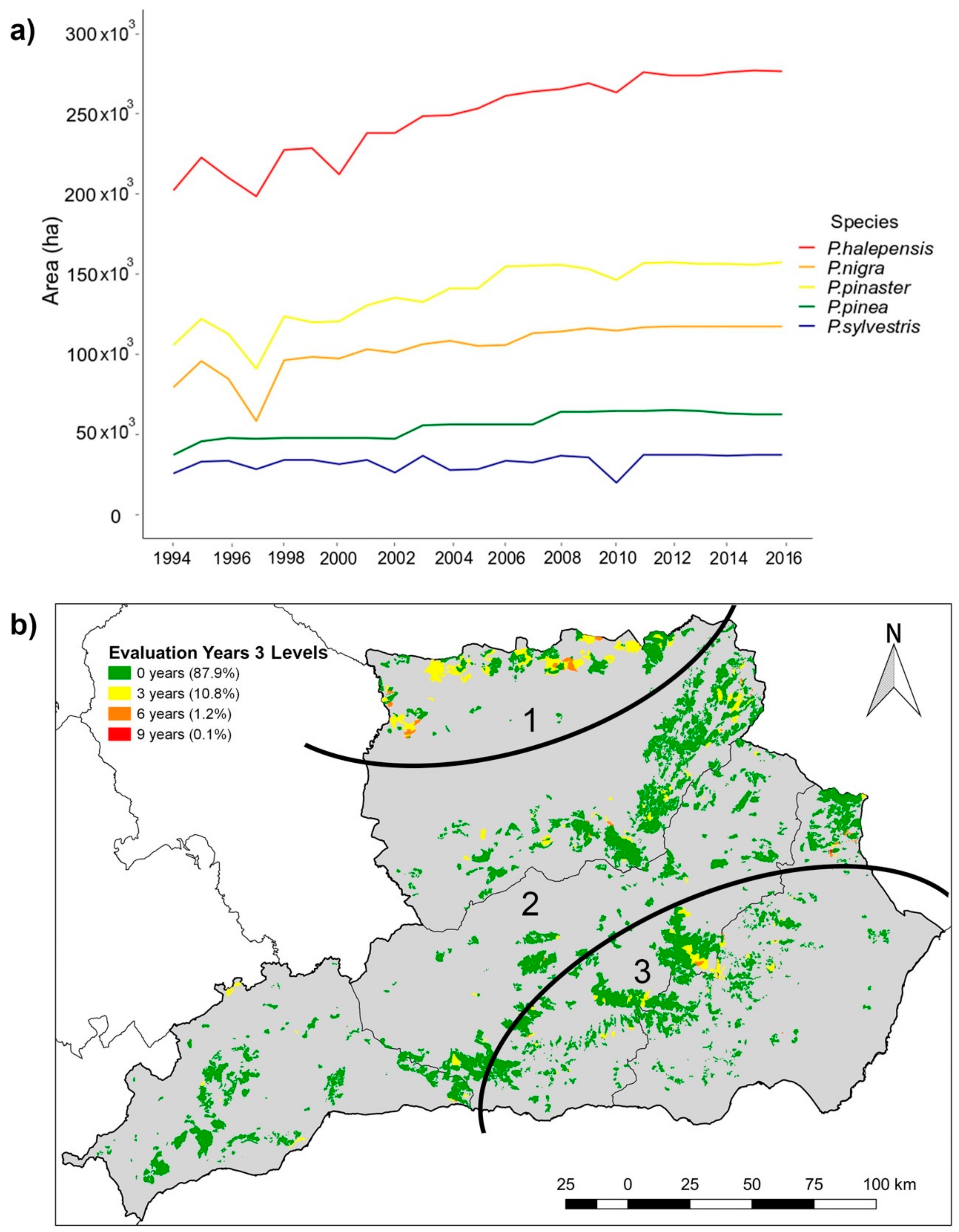
2.1. Insect Outbreak Area

The study area is located in the southeastern of Spain (37°26′08.4″ N 2°51′32.5″ W, WGS-84), more specifically in eastern Andalusia, covering the provinces of Almería, Granada, Jaén, and Málaga. This area is made up of 3147 stands, in which five Pinus species (P. halepensis, P. pinea, P. pinaster, P. nigra, and P. sylvestris) were selected and multi-year forest defoliation was monitored across different ecological settings (Figure S1, Table S1, Supplementary Material). Arranged from the lower elevation areas of P. halepensis to the higher elevation areas of P. sylvestris, pure or mixed stands are found, many of them being forest plantations established in the 1970s, with the inclusion of some natural stands. The area covers a wide variety of environmental conditions, but a dry Mediterranean climate dominates most of the forests. This climate is characterized by hot summers and warm winters, unlike the humid Mediterranean climate, which has mild summers and winters, due to the influence of the sea. The annual rainfall ranges from 200 to 600 mm and the mean annual temperature is 12.1 °C, according to the location and elevation. The topography is characterized by steep mountains to the southeast, and the elevation range is between 0 and 1900 masl.

2.2. Defoliation Data Selection and Quality Control

In annual monitoring campaigns, maps of the PPM at the forest stand scale from 1994 to 2016 were produced using established ground survey sketch mapping techniques by the Junta de Andalusia Forest Service, as part of the Integrated Control Plan of the PPM. These PPM data are used to estimate the spatial extents of areas disturbed by the PPM, and as additional information to identify if those pine stands have had silvicultural treatments (e.g., thinning). Forest defoliation is estimated every year using the approach established by Montoya and Hernández (1991). Each individual stand is observed by eye, or with binoculars when necessary, and the defoliation level is assessed during February-March. This period is preferred because sighting and identification of host trees are easier. The stands are then classified into six visual levels of defoliation [16], which have been grouped in this study into three defoliation levels because damages showed similarities. Moreover, the sample size of high levels of damage increased to facilitate the statistical process (Table S2, Supplementary Material). Once the information had been compiled, it was necessary to refine the raw data and organize the selected data into a reliable database. In order to conduct statistically reliable analyses of the defoliation data, the only stands considered were those from plots that had been continuously sampled for at least 22 years and that had not received silvicultural treatments. These data were originally given as vector polygons outlining the forest stands, having data on the tree species fraction and development stage (age class). The forest stand map was resampled to a raster with a 30-m resolution for use with Landsat data. The degree of defoliation varied within the area from no to almost complete defoliation.

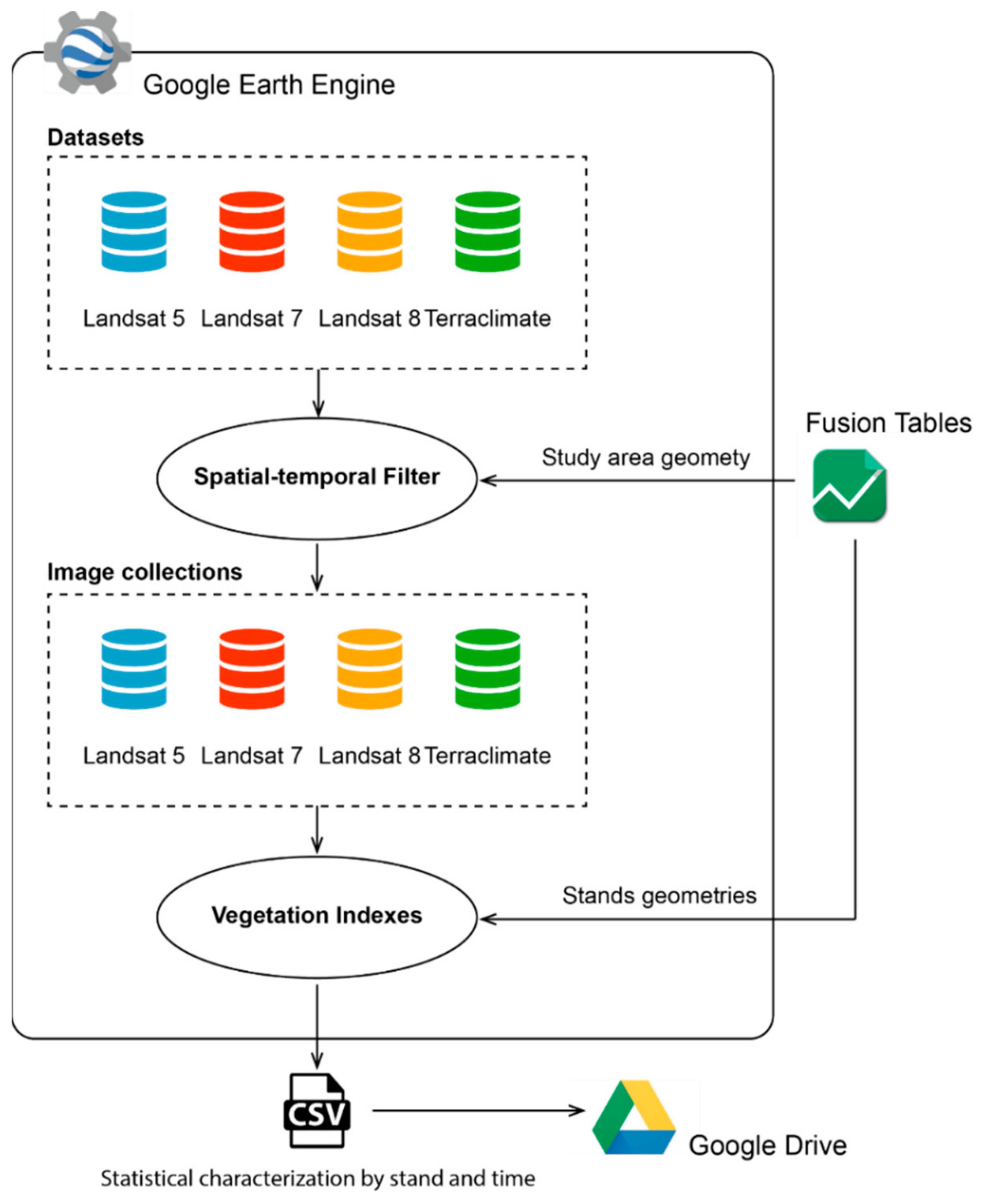
2.3. Datasets and Image Processing

Data preparation and processing were performed with Google Earth Engine (GEE). Earth Engine Python API was used as the client library to interact with Earth Engine Servers, using the Python programming language. Figure 1 summarizes the remote sensing processing.

Full spatial-temporal coverage of Landsat scenes for the period 1994–2016, between February and March, was used for this study. A total of 1148 Landsat images with bottom of atmosphere (BOA) reflectance, at 30-m spatial resolution, were used; of these, 532 images were registered by Landsat Thematic Mapper (TM, 1994–2011), 517 were from Enhanced Enhanced Thematic Mapper (ETM+, 1999–present), and 99 from Operational Land Imager (OLI, 2013–present). The TM and ETM+ images are distributed after atmospheric correction using the Landsat Ecosystem Disturbance Adaptive Processing System (LEDAPS) [40] and included a cloud, shadow, water, and snow mask produced using the C Function of Mask (CFMASK) [41,42], as well as a per-pixel saturation mask. The OLI images were distributed after atmospheric correction using Landsat 8 Surface Reflectance Code (LASRC). Moreover, a spatial filter was applied to exclude those images with a footprint that failed to intersect a geometry delimiting the area of interest. This geometry was uploaded from a KML file to Fusion Tables.

Four vegetation indexes (VIs) were calculated for each singular image: the Normalized Difference Vegetation Index (NDVI), Moisture Stress Index (MSI), Normalized Difference Infrared Index (NDII), and Ratio Vegetation Index (RVI) (Table S3, Supplementary Material). These four VIs have proven effective according to the remote sensing defoliation assessment literature [22]. The NDVI index was used since it has been related successfully to leaf pigments and defoliation, but it was insensitive to biomass changes. To avoid this problem, we also tested other sensitive VIs. The MSI is related to the water in cellular structures and to plant vigor by using the SWIR and NIR bands [43]. High values of MSI mean low vigor and high water stress [43]. Based on the same spectral bands, the NDII index calculated the normalized difference between the NIR and SWIR bands [44] and has been used to detect vegetation water stress during drought periods [45]. Finally, we used RVI, which is widely used for green biomass estimations, specifically, at high-density vegetation coverage, since it is very sensitive to vegetation structure and has a good correlation with plant biomass [46].

The VIs were calculated considering two different polygonal geometries, one inside the stand area and the other defining a 60-m buffer around the perimeter of the stand (Figure S2, Supplementary Material), and each singular stand area was characterized by the average value of the VIs.

2.4. Environmental Variables

Climatic variables from the Terraclimate database were collected. This database comprises monthly climate and climatic water balance data for global terrestrial surfaces. It uses climatically aided interpolation, combining high-spatial-resolution climatological normal data from the WorldClim dataset and the Japanese 55-year Reanalysis (JRA55) [47]. The variables obtained from this database were the maximum and minimum monthly temperatures, monthly precipitation, and monthly radiation for the period 1994–2016.

Together with the TerraClimate data, environmental data layers were also downloaded from the Andalusia Environmental Information Network (REDIAM) http://www.juntadeandalucia.es/medioambiente/site/rediam/portada/. The dataset (47 variables) contains four categories of variables: 11 climatic variables, 17 edaphic variables, 15 topographic variables, and four tree cover variables (Table S4, Supplementary Material).

2.5. Statistical Analysis

Prior to statistical analysis, the normality and homoscedasticity were analyzed using the Kolmogorov-Smirnov test and Levene test of variance (p > 0.05), respectively. The VIs were analyzed with a one-way ANOVA test, considering the overall and 60-m buffer stand values. When a global difference among damage levels was detected, means were separated by Scheffe’s multiple range test for unequal sample sizes (p = 0.05), for normal and homoscedastic variables [48].

Once the best index was selected, we assumed that the annual time-series of defoliation levels, expressed through the VI selected, could be spatially synchronized., as if they were tree growth rings, using the computer program COFECHA [49] and according to the methodology already used in other defoliation analyses to obtain significant temporal correlation patterns [50]. We obtained a master chronology of sample defoliation level. eliminating autoregression by using moving average techniques in two stages. An initial synchronization analysis considering all species showed whether there was a significant common signal of spatial correlation between the PPM damage time series. The set of interspecific stands that gave a positive response to the first synchronization (S1) underwent a second synchronization analysis to detect a significant intraspecific spatial response among the five Pinus species studied (S2). The stands associated with a synchronized response provided an overall territorial response to a common signal.

The relationship between the master standardized indexes synchronized stands (S2) and the environmental variables of each stand was studied using the k-Nearest Neighbor (kNN) machine-learning algorithm [51,52]. Explanatory variables were selected firstly by using variance inflation factor (VIF) analysis to check multicollinearity, and secondly by choosing the variable or combination of variables which minimized the generalized root mean square distance when variables were added or deleted one at a time [53]. Thus, once the best predictor variables had been selected, we used random forest (RF) to establish the relationships with the NDII values of the synchronized stands (S2). We estimated the accuracy of the kNN predictions by external validations, using, at random, 60% of the data for training and 40% for evaluation, and by calculating the bias and Root Mean Square Error (RMSE) values of the model.

We performed all analyses using R software, version 3.4.0. (R Development Core Team, 2012). The yaImpute R package was used for variable selection and regression with kNN [54], the lm and glm function of MASS library were used for ANOVAs [55], the usdm package was used to perform collinearity analysis and VSURF package was used to implement the Random Forest variable selection [56].

3. Results

3.1. Defoliation of Individual Species

Southeastern Spain has been impacted for the last 22 years by the prolonged defoliation of pine trees provoked by the PPM. The five species studied here (P. halepensis, P. nigra, P. pinaster, P. pinea, and P. sylvestris) had different areas affected by defoliation in each year (Figure 2a; Table S5, Supplementary Material): P. halepensis was the species most affected, followed by P. pinaster, P. nigra, P. pinea, and P. sylvestris, respectively. When all stands were considered, there was a trend of increasing defoliation over the period 1994–2016, with the maximum value occurring in 2016 (Figure 2a). Defoliation of P. halepensis, P. nigra, and P. pinaster was lower in the period 1996–2000 but increased gently from 2001 to 2016 (Figure 2a). The temporal analysis suggests that the defoliation of these species by the PPM experimented a slight increase, with a number of stands never recovering their original condition, and the average percentage defoliation remained higher until 2016 (Figure 2a). The defoliation pattern exhibited by P. sylvestris and P. pinea was similar, although mildly less marked, particularly regarding the maximum and minimum values reached. In both species, the percentage defoliation values of stands increased at a very low rate over the 22-year monitoring period. Figure 2b shows the spatial distribution and temporal evolution of the affected area at level 3. In general, most of the stands have less than 3 years at level 3 however, northern and southern areas are stands with more than 6 years at level 3.

The annual area affected by each level of defoliation (Table S5, Supplementary Material) shows that the dominant defoliation level for all species was level 1, followed by level 2 and low presences in some years of level 3. In addition, level 3 was more frequent in some species, such as P. halepensis. There are also indications of cyclic behavior of the PPM in the time series, with areas affected by levels 2 and 3 increasing in 1998, 2004, 2009, and 2016. In 2016, a dramatic increment in level 3 was observed for most species, this being the year with the greatest area showing this level of defoliation in the whole series.

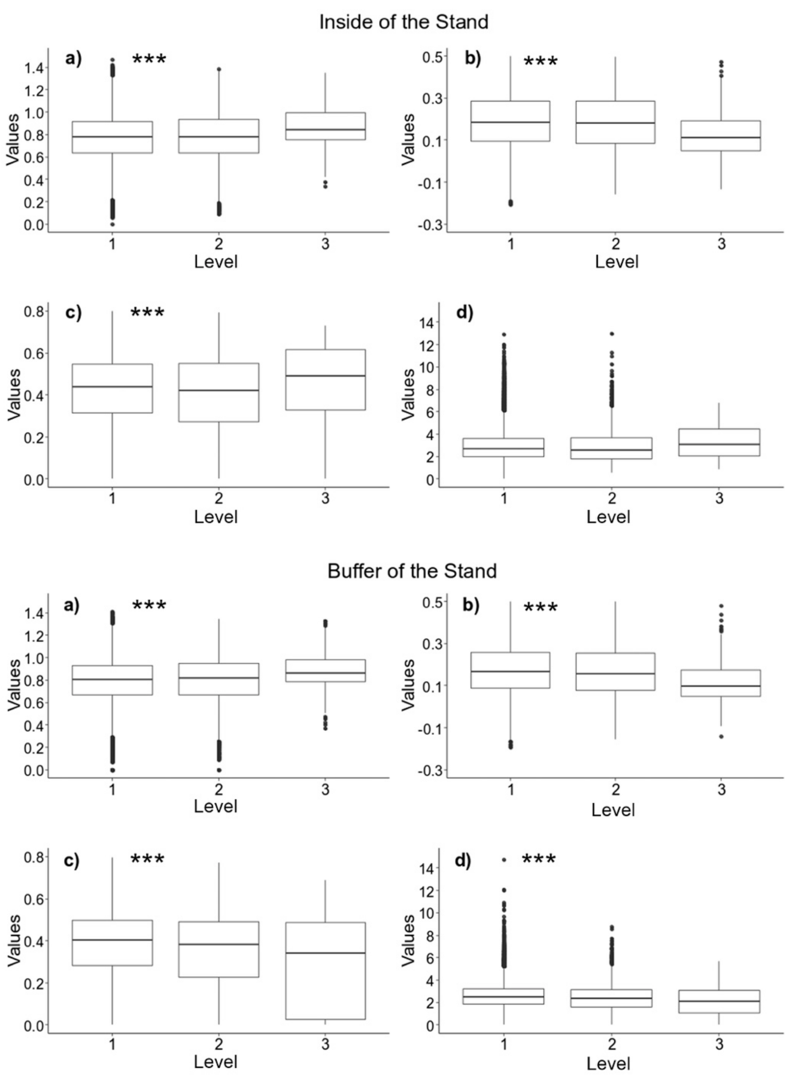
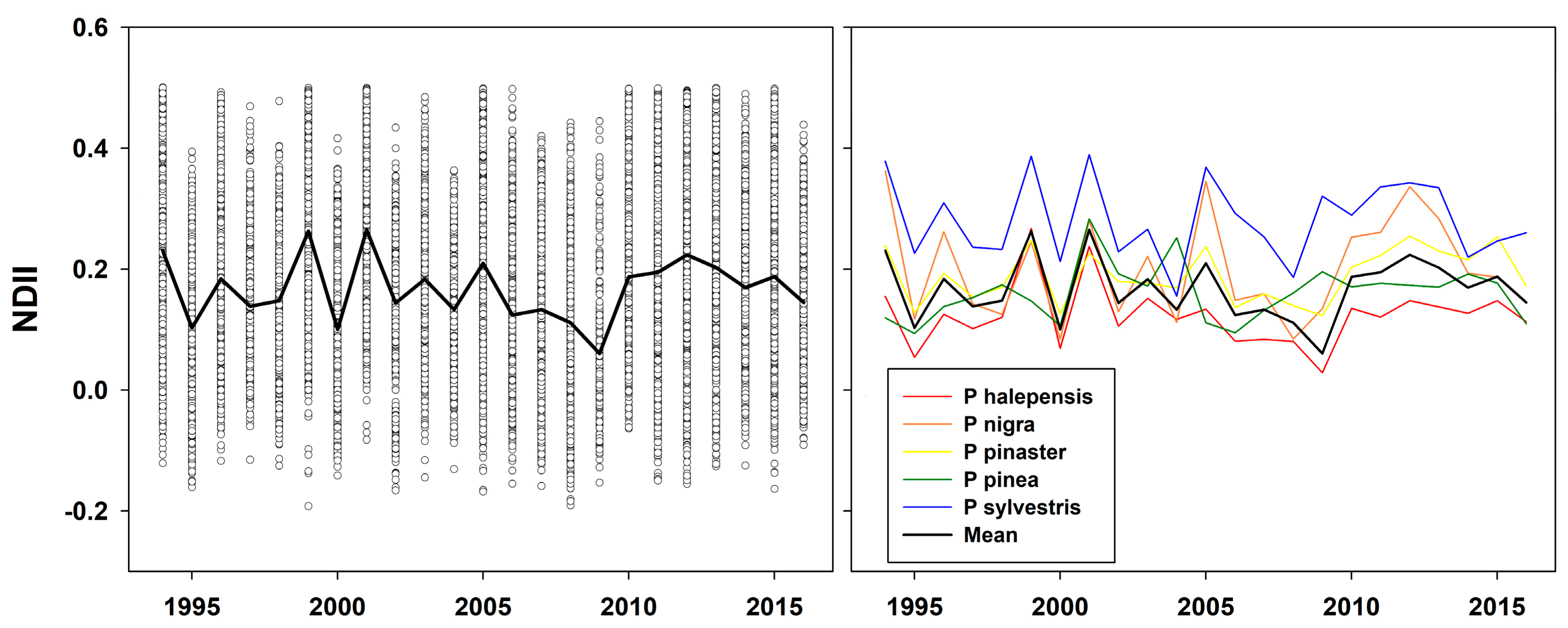
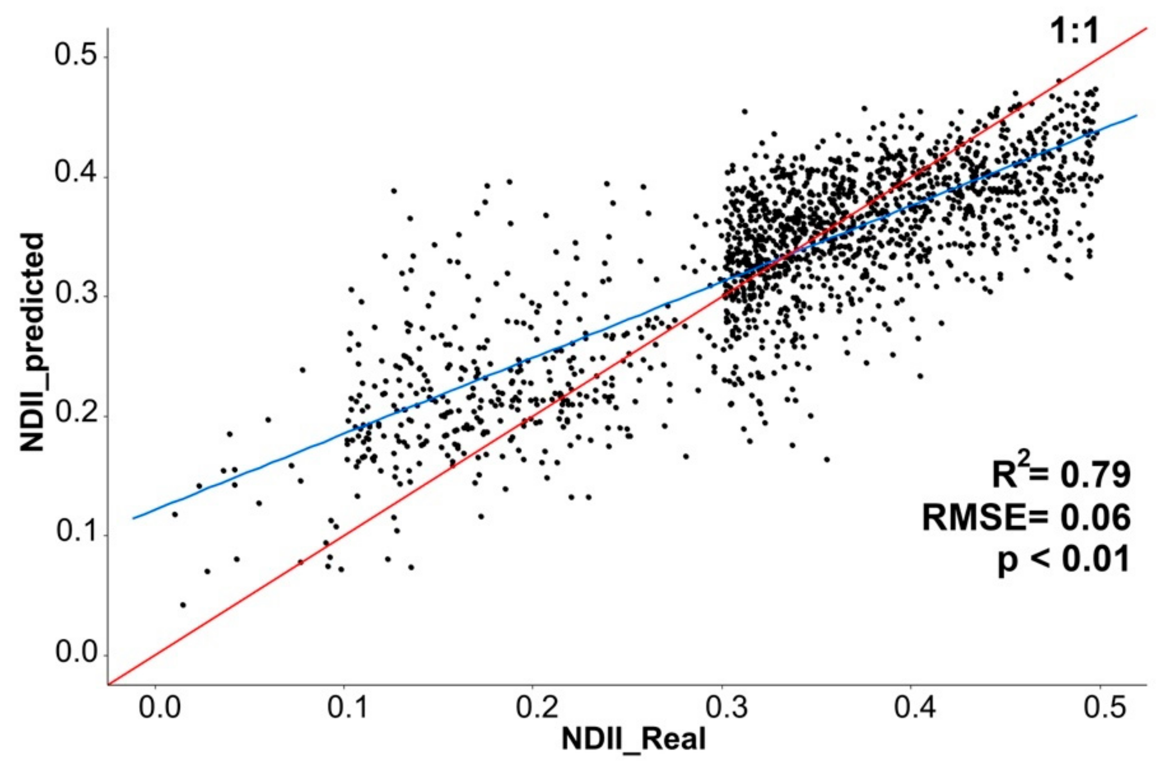
3.2. Vegetation Indexes

The results of the univariate ANOVA for all VIs are summarized in Figure 3. The average values of the indexes for the entire time series, according to the levels of defoliation, were practically equal when considering the area inside the stand and in the 60-m buffer (Table S6, Supplementary Material). The MSI value was greater (significantly so) for the highest defoliation level (p < 0.001), for both areas, while NDII showed an inverse response (p < 0.001). The NDVI and RVI indexes increased significantly with the defoliation level, although the differences were not significant for the 60-m buffer stands in the case of RVI (p = 0.124; Table S6, Supplementary Material). Therefore, the best VIs with regard to the estimation of PPM defoliation were MSI and NDII, for both the overall and 60-m buffer stands. Finally, the buffer values of NDII were selected to assess PPM defoliation because they showed the greatest differences between the average values of the degrees of defoliation (Figure 3; Table S6, Supplementary Material).

3.3. Synchronization and Defoliation Patterns

Based on the defoliation calculated using NDII (hereafter defoliation-NDII), the defoliation synchronization analysis was performed in the 3147 PPM stands. It included the five species and the continuous defoliation time series available for a period of 22 years (Figure 4;

Table 1. Number of stands per species with defoliation related to a processionary moth for the time series 1994–2016 and related statistics based on the autoregressive model used in the analysis of the synchrony of the NDII-defoliation process.

Species	N	R12	MS
P. halepensis	977	0.556	0.467
P. nigra	419	0.804	0.533
P. pinaster	480	0.467	0.268
P. pinea	227	0.532	0.234
P. sylvestris	200	0.612	0.268
Pinus sp.	3147	0.515	0.384

N: number of stands with defoliation timeseries 1994–2016 years; R₁²: intraspecific correlation; MS: model mean sensitivity.

). The result obtained for all the species considered together showed a positive spatiotemporal correlation (S1). A second analysis was conducted (in S1 stands with a correlation of defoliation series ≥ 0.5, N = 2303) to examine spatial synchronization among the stands of each Pinus species. The defoliation pattern exhibited by the individual species synchronization (S2) was similar to the S1 response, although mildly more marked, particularly regarding the maximum and minimum values reached (Figure 4; Table 1)

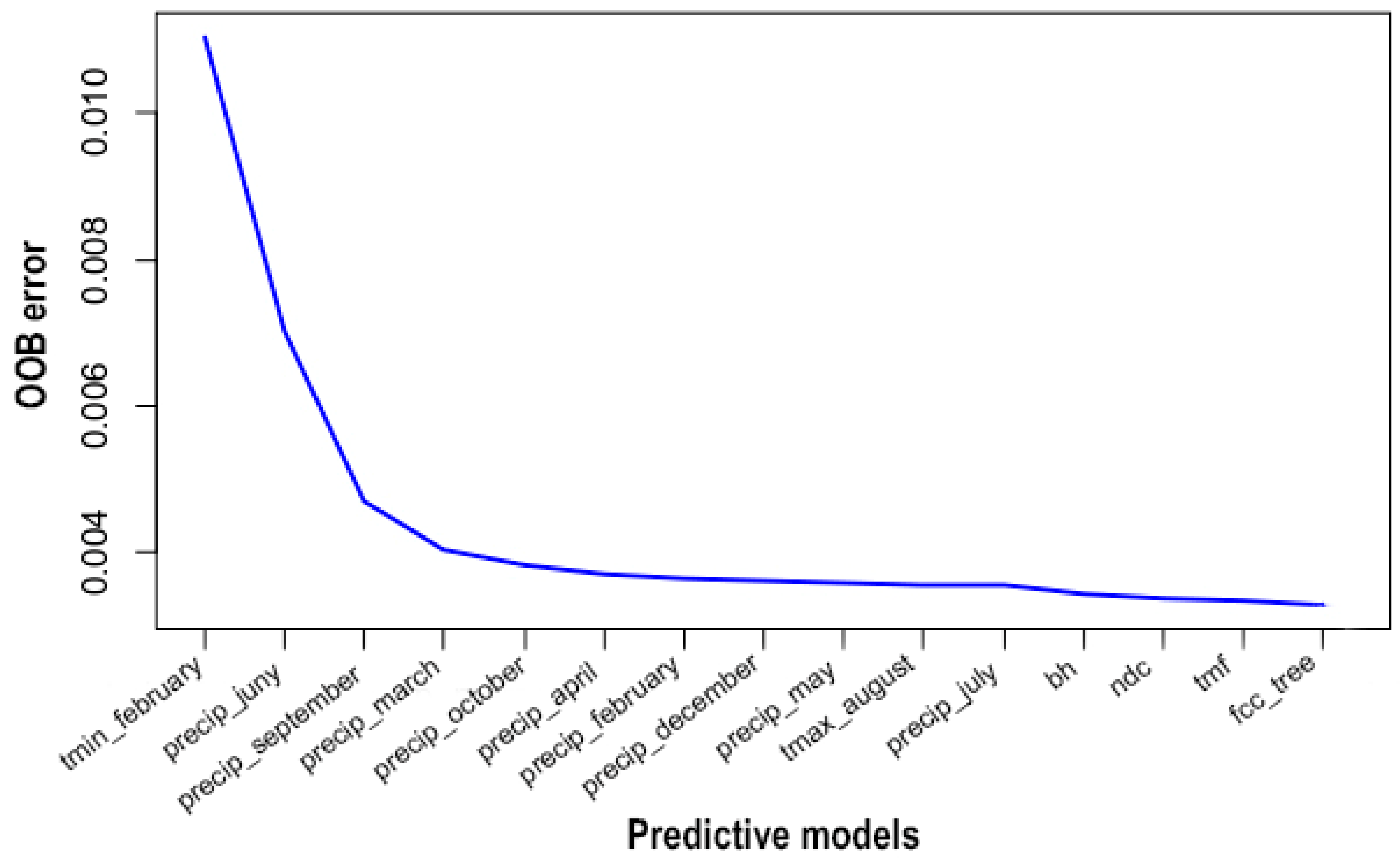
3.4. Environmental Predictors

Investigation of how the specific NDII-defoliation responded as a function of the environmental conditions may help to predict the potential impacts of the PPM. Up to 47 environmental variables were used to perform RF regression and, following a sparsity test of the predictor matrix, NDII-defoliation was related to 30 environmental variables (Figure 5; Table S4, Supplementary Material), given their importance in driving PPM defoliation. According to the RF model generated, variables related to the thermal and precipitation regime, such as the minimum temperature of February and the seasonal precipitation (June, September, March, and October), showed the highest values of importance. The predictor variables related to soil and silvicultural characteristics had moderate importance with regard to NDII-defoliation levels (Figure 5).

We computed the scatter plots for correlations contrasting the observed and estimated values for all NDII-defoliation predictions (Figure 6). The correlations obtained were highly significant (R² = 0.79, RMSE = 0.06%; Table S7, Supplementary Material).

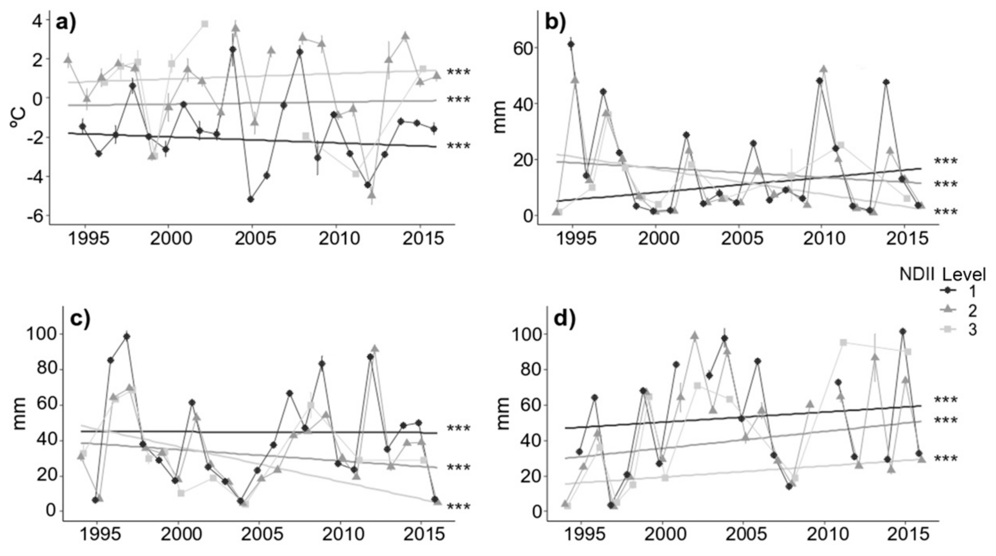
3.5. Temporal Trends

Finally, we evaluated the temporal trends of the RF variables according to the PPM defoliation. Levels 2 and 3 increased with the rise in winter temperature (Figure 7a) and the decrease in average summer precipitation (June and September; Figure 7b,c). An increase in mean spring precipitation (March) produced a slightly significant deviation in the defoliation patterns (Figure 7d). The regression models relating environmental drivers and PPM defoliation levels indicated that warm winters and dry summers were the most important predictors of this defoliation.

4. Discussion

In this study, we confirmed the potential of using spatial medium-resolution Landsat time-series data to assess the spatiotemporal patterns of pine defoliation caused by the PPM in Andalusia (southeastern Spain). The method applied here allowed us to integrate field and Landsat data for the analysis and interpretation of the ecological drivers of PPM damage, and to develop a fully operational system for monitoring insect damage through a combination of field and remote sensing data from different sources.

4.1. Defoliation of Individual Species

We found a substantial increase in the area defoliated by the PPM, based on the field survey in the area mapped as defoliated along the years 1994 to 2016. During this time, the study area underwent a significant increase in PPM defoliation for all species, in particular for P. halepensis, P. pinaster, and P. nigra forests. These species also had the greatest extension cover, P. halepensis being the most representative species of pine in Andalusia [57]. The distribution of the distinct defoliation levels was practically equal for all species, although levels 2 and 3 showed a cyclical character. This may be related to the phenology of the PPM, which tends to have stronger outbreaks every 4–5 years [9,58]. However, this increase in PPM defoliation might also be a result of other factors—such as the climate, which has both a direct influence, on tree physiology, and an indirect effect, on the defoliating species [4,59]. It is also possible that the field-overview survey detected a resurgence of other defoliation processes that could not be captured by visual observation; including multiple disturbances within field time series. Another relevant result was the high increase in levels 2 and 3 since 2014, in all species, 2016 being the year with the highest recorded values. This implies that defoliation due to the PPM will increase in the coming years, causing more concern for forest managers. In addition, we can assume that all pine species in this area are currently endangered by defoliation. This should be highlighted, since in previous works a preferable choice of certain pine species was mentioned, where PPM in the Mediterranean has changed host because it has expanded its altitudinal range of distribution, primarily due to climate change [4,14].

4.2. Vegetation Indexes

We assessed the occurrence of PPM defoliation using four Landsat-derived vegetation indexes—MSI, NDII, NDVI, and RVI—which greatly facilitate the estimation of defoliation at the regional scale. The four indexes analyzed showed different responses to defoliation, MSI and NDII having the most significant relationships. Consequently, a method for estimating the degree of PPM defoliation based on these relationships was reached. The indexes had opposing relationships with defoliation: MSI was the most affected, having greater values as water stress increased, and the values of NDII decreased as the level of damage rose since the most affected areas perform less photosynthesis. For easier comparison with other work, and because the behavior of MSI in forests has not yet been adequately investigated, we suggest the use of NDII to assess PPM defoliation. Several studies have demonstrated the importance of information from SWIR bands for forest disturbance and insect damage detection [25,60,61]. Therefore, NDII was selected as the best index because it is a green assessment index and showed a greater range of separability between defoliation levels. In addition, it exhibited significant differences in the two statistical tests performed, for both the interior and perimeter zones. However, several gridding artefacts—such as forest structure (e.g., differences in understory vegetation, clear-cuts, and thinning) or image quality (e.g., the influences of the clouds, atmosphere, sun, and view angles on the Landsat data)—could introduce errors in the spatial accuracy of the VIs values, which may lead to overestimation of the mapped damage areas [62]. However, some of these effects were smoothed by checking and removing the thinning areas that were present in the PPMS maps, to reduce the effects of structural changes [63].

A further problem is the separation of the area inside the stand from that of the 60-m buffer, because of the medium spatial scale of the Landsat data. This differentiation between internal and buffer areas has been widely used in previous studies [7,22], as the perimetral area is damaged more by the PPM [16]. Our results revealed that the differences between the VIs values in the internal areas and those of the 60-m buffer areas were significant for levels 1 and 2. However, the level 3 values were practically identical, which can be explained because in these stands all the surface area was completely affected. As a consequence, considering only the area inside the stand might lead to underestimation of the real damage, because the perimeter zone is more affected than the internal one. This can be explained because the field survey polygons might have contained multiple small areas with uninfected or mildly defoliated patches which were considered broad areas with similar defoliation levels rather than fine-scale defoliation impacts. It makes sense to select the 60-m buffer area of the stand to avoid overestimates of the total area defoliated—as have been observed in previous research, especially when mapping areas with low levels of defoliation [7].

4.3. Environmental Variables Associated with the PPM

This research used the temporal series of defoliation-NDII data along 22 consecutive years, as presented in previous dendrochronological work, to study the synchrony of the PPM [50]. The synchronization of the NDII-defoliation data gave a similar pattern for the Pinus species when considered together and individually, showing the ability of this index to adjust model parameters based on the characteristics of specific defoliation levels. Based on these series, we explored the synergies and relationships between environmental factors that lead to defoliation by the PPM.

Landsat-derived temporal patterns of PPM levels in Andalusia varied significantly with climatic and environmental patterns. In this study, according to the RF model, defoliation trends were associated with the temperatures in February and June and the precipitation in September. The minimum temperature in February influenced the PPM by lengthening or shortening the larval phase of the species, making annual defoliation longer or shorter, respectively, and leading to different levels of defoliation severity ([15]; Figure S3, Supplementary Material). When there is an increase in the minimum temperature, a greater grouping of individuals allows them to withstand these extreme temperatures. In general, our results confirm the relevant effect of moisture stress as an important trigger of the PPM population, based on seasonal variations in the temperature, precipitation, and drought patterns [64]. In addition, summer precipitation may be related to the plant stress hypothesis [65], which states that moderate drought stress enhances the foliar concentrations of sugars and nutrients favoring the survival, growth, and reproduction of larvae [66]. Here, the period of lower than average summer and early autumn precipitation might have caused such drought stress in the primary hosts of the PPM—Pinus spp.—which are sensitive to autumn precipitation deficits. In addition, the September precipitation influences several phases of the PPM. It prolongs or shortens the adult phase, affecting the number of offspring for the next generation, as well as influencing the number and size of eggs. As the temperature decreases, the eggs become smaller and more abundant in the clutches [59], making the next generation more numerous and therefore producing more defoliation. However, the environmental influences on the occurrence of PPM outbreaks—as the factors determining the synchrony between Mediterranean Pinus species and larval phenology—are highly complex and depend on many other factors not considered here, such as the chemical defense induced by each species against defoliants. or the biotic enemies of the PPM [64], which should be included in future studies.

4.4. Temporal Trends

Regarding the trends in the defoliation level related to environmental variables, as the February temperature increased, the occurrence of PPM defoliation levels 2 and 3 sharply increased, although the trends of all levels showed low r-square values, due to the great dispersion of the defoliation values. The significantly lower than average summer precipitation during the temporal series might also be associated with drought stress in Mediterranean Pinus species [67]—thus benefiting larval development, as discussed earlier. This has been found in several previous studies reporting the coincidence of PPM outbreaks with dry periods [64]. In a dendrochronological study, [7] described the cycled response of PPM to rain periods following by drought which promote PPM population growth. During favorable years, foliage quantity and quality prevent stands collapse due to starvation even when PPM levels are high. On the other hand, despite the fact that moderate drought stress can stimulate PPM population growth initially, severe drought (e.g., those observed during the last years in southern Spain, [68]) might have led to the observed PPM outbreak and its subsequent collapse (i.e., the increment damages after 2010; Figure 7) following the accumulative dry summers after 2003.

4.5. Limitations and Uncertainties

Although our interpretations of the spatiotemporal patterns of the PPM are very encouraging, the methods developed exhibit some constraints. This study used a temporal series of multiple outbreaks of the PPM in Andalusia related to field-survey data, which can correspond to local relationships between the climate and PPM outbreak patterns. In fact, the observed relationships confirm previous results based on dendrochronological studies [7], pointing out the strong influence of the climate on PPM outbreak dynamics. Another limitation is that our work is focused especially on one important factor (climate) although other factors like land use or predatory-prey systems [2] or should be taken into account in future research projects. Finally, the defoliation due to the PPM was identified using Landsat analysis when the PPM populations had already become large enough to produce a level of defoliation visible in Landsat images. Future work should involve datasets spanning several scales (namely, field data and remotely sensed data) to deepen our comprehension of the complicated ecological processes determining PPM outbreaks [69], providing useful insights into the dynamics of PPM damage and fresh evidence to support earlier suggestions and predictions from work focused on remote sensing, field surveys, and simulation modeling.

5. Conclusions

This study used Landsat temporal series to describe the levels of defoliation due to the PPM in Pinus forests of southeastern Andalusia. The utilization of GEE as a platform to calculate VIs from image collections, from which pixel values were extracted for each of the forest stand polygons, was efficient and effective. Our results confirm the potential for using Landsat time-series data for the assessment of PPM defoliation, although key uncertainties remain. We have used a system based on a combination of remotely sensed data and field survey data to detect and classify the defoliation levels of different Pinus spp. All the Pinus species tested are affected by PPM defoliation, with a cyclic behavior that has increased in recent years. The defoliation levels were practically equal for all species, with a high increase in defoliation levels 2 and 3 since 2014, 2016 being the year with the highest recorded values. The MSI and NDII vegetation indexes exhibited overall accuracies similar to those of other studies that used these indexes to assess defoliation due to the PPM. The synchronization of the NDII-defoliation data had a similar pattern for all and individual Pinus species, showing the ability of this index to adjust model parameters based on the characteristics of specific defoliation levels. Using Landsat-based NDII-defoliation maps and interpolated environmental data, we have shown that the PPM defoliation in Southern Spain is driven by the minimum temperature in February and the precipitation in June, March, September, and October, through their influence on the biological development of the PPM. Therefore, the NDII-defoliation assessment seems to be a general index that can be applied to forests in other areas. The trends in the defoliation level in relation to environmental variables showed the importance of summer drought stress in the expansion of the PPM on Mediterranean Pinus species. The use of Landsat time-series data of medium spatial resolution to assess the spatiotemporal patterns of defoliation caused by the PPM is a powerful tool to assess and analyze the ecological drivers of PPM outbreaks and to develop a fully operational system for the monitoring of insect damage, using a combination of field and remote sensing data from different sources.

References

1. Pemán García, J.; Iriarte Goñi, I.; Lario Leza, F.J. La Restauración Forestal de España: 75 Años de una Ilusión; Ministerio de Agricultura y Pesca, Alimentación y Medio Ambiente: Madrid, Spain, 2017; ISBN 978-84-491-1495-3.
2. Raffa, K.F.; Aukema, B.; Bentz, B.J.; Carroll, A.; Erbilgin, N.; Herms, D.A.; Hicke, J.A.; Hofstetter, R.W.; Katovich, S.; Lindgren, B.S.; et al. A Literal Use of “Forest Health” Safeguards against Misuse and Misapplication. J. For. 2009, 107, 276–277. [Google Scholar]
3. Gandhi, K.J.K.; Herms, D.A. Direct and indirect effects of alien insect herbivores on ecological processes and interactions in forests of eastern North America. Biol. Invasions 2010, 12, 389–405. [Google Scholar] [CrossRef]
4. Netherer, S.; Schopf, A. Potential effects of climate change on insect herbivores in European forests—General aspects and the pine processionary moth as specific example. For. Ecol. Manag. 2010, 259, 831–838. [Google Scholar] [CrossRef]
5. Lakatos, F.; Mirtchev, S.; Mehmeti, A.; Shabanaj, H. Handbook of the Major Forest Pests in South East Europe; Food and Agriculture Organization of the Unitednations: Pristina, Serbia, 2014; p. 117. [Google Scholar]
6. Senf, C.; Seidl, R.; Hostert, P. Remote sensing of forest insect disturbances: Current state and future directions. Int. J. Appl. Earth Obs. Geoinf. 2017, 60, 49–60. [Google Scholar] [CrossRef] [PubMed] [Green Version]
7. Sangüesa-Barreda, G.; Camarero, J.J.; García-Martín, A.; Hernández, R.; de la Riva, J. Remote-sensing and tree-ring based characterization of forest defoliation and growth loss due to the Mediterranean pine processionary moth. For. Ecol. Manag. 2014, 320, 171–181. [Google Scholar] [CrossRef] [Green Version]
8. Kapeller, S.; Schroeder, H.; Schueler, S. Modelling the spatial population dynamics of the green oak leaf roller (Tortrix viridana) using density dependent competitive interactions: Effects of herbivore mortality and varying host-plant quality. Ecol. Model. 2011, 222, 1293–1302. [Google Scholar] [CrossRef]
9. Li, S.; Daudin, J.J.; Piou, D.; Robinet, C.; Jactel, H. Periodicity and synchrony of pine processionary moth outbreaks in France. For. Ecol. Manag. 2015, 354, 309–317. [Google Scholar] [CrossRef]
10. Dudley, T.L.; Bean, D.W. Tamarisk biocontrol, endangered species risk and resolution of conflict through riparian restoration. BioControl 2012, 57, 331–347. [Google Scholar] [CrossRef]
11. Kautz, M.; Meddens, A.J.H.; Hall, R.J.; Arneth, A. Biotic disturbances in Northern Hemisphere forests—A synthesis of recent data, uncertainties and implications for forest monitoring and modelling. Glob. Ecol. Biogeogr. 2017, 26, 533–552. [Google Scholar] [CrossRef]
12. Meng, R.; Dennison, P.E.; Zhao, F.; Shendryk, I.; Rickert, A.; Hanavan, R.P.; Cook, B.D.; Serbin, S.P. Mapping canopy defoliation by herbivorous insects at the individual tree level using bi-temporal airborne imaging spectroscopy and LiDAR measurements. Remote Sens. Environ. 2018, 215, 170–183. [Google Scholar] [CrossRef]
13. Kirilenko, A.P.; Sedjo, R.A. Climate change impacts on forestry. Proc. Natl. Acad. Sci. USA 2007, 104, 19697–19702. [Google Scholar] [CrossRef] [PubMed] [Green Version]
14. Hódar, J.A.; Zamora, R.; Cayuela, L. Climate change and the incidence of a forest pest in Mediterranean ecosystems: Can the North Atlantic Oscillation be used as a predictor? Clim. Chang. 2012, 113, 699–711. [Google Scholar] [CrossRef]
15. Roques, A.; Rousselet, J.; Avcı, M.; Avtzis, D.N.; Basso, A.; Battisti, A.; Jamaa, M.L.B.; Bensidi, A.; Berardi, L.; Berretima, W.; et al. Climate Warming and Past and Present Distribution of the Processionary Moths Thaumetopoea spp. in Europe, Asia Minor and North Africa. In Processionary Moths and Climate Change: An Update; Springer: Dordrecht, The Netherland, 2015; pp. 81–161. ISBN 978-94-017-9339-1. [Google Scholar]
16. Montoya; del Pino, H.P. Informaciones Técnicas Departamento de Medio Ambiente del Gobierno de Aragón. 1998. Available online: http://www.caib.es/sites/sanitatforestal/f/23622 (accessed on 29 April 2019).
17. Démolin, G. Bioecologia de la procesionaria del pino Thaumetopoea pityocampa Schiff. Incidencia de los factores climáticos. Bol. Serv. Plagas For. 1969, 23, 9–24. [Google Scholar]
18. Consejeria de Medio Ambiente y Ordenación del Territorio Plan de Lucha Integrada Contra la Procesionaria del Pino. 2003, p. 43. Available online: http://www.juntadeandalucia.es/medioambiente/site/portalweb/menuitem.7e1cf46ddf59bb227a9ebe205510e1ca/?vgnextoid=1815e6f1563d6510VgnVCM1000001325e50aRCRD&vgnextchannel=d9cfe6f1563d6510VgnVCM1000001325e50aRCRD (accessed on 29 April 2019).
19. De Beurs, K.M.; Townsend, P.A. Estimating the effect of gypsy moth defoliation using MODIS. Remote Sens. Environ. 2008, 112, 3983–3990. [Google Scholar]
20. Pause, M.; Schweitzer, C.; Rosenthal, M.; Keuck, V.; Bumberger, J.; Dietrich, P.; Heurich, M.; Jung, A.; Lausch, A. In Situ/Remote Sensing Integration to Assess Forest Health—A Review. Remote Sens. 2016, 8, 471. [Google Scholar] [CrossRef]
21. Rullan-Silva, C.D.; Olthoff, A.E.; de la Mata, J.A.D.; Pajares-Alonso, J.A. Remote Monitoring of Forest Insect Defoliation—A Review. For. Syst. 2013, 22, 377–391. [Google Scholar] [CrossRef]
22. Zhu, C.; Zhang, X.; Zhang, N.; Hassan, M.A.; Zhao, L. Assessing the Defoliation of Pine Forests in a Long Time-Series and Spatiotemporal Prediction of the Defoliation Using Landsat Data. Remote Sens. 2018, 10, 360. [Google Scholar] [CrossRef]
23. Belgiu, M.; Drăguţ, L. Random forest in remote sensing: A review of applications and future directions. ISPRS J. Photogramm. Remote Sens. 2016, 114, 24–31. [Google Scholar] [CrossRef]
24. Wulder, M.A.; Dymond, C.C.; White, J.C.; Leckie, D.G.; Carroll, A.L. Surveying mountain pine beetle damage of forests: A review of remote sensing opportunities. For. Ecol. Manag. 2006, 221, 27–41. [Google Scholar] [CrossRef]
25. Goodwin, N.R.; Coops, N.C.; Wulder, M.A.; Gillanders, S.; Schroeder, T.A.; Nelson, T. Estimation of insect infestation dynamics using a temporal sequence of Landsat data. Remote Sens. Environ. 2008, 112, 3680–3689. [Google Scholar] [CrossRef]
26. Wang, C.; Lu, Z.; Haithcoat, T.L. Using Landsat images to detect oak decline in the Mark Twain National Forest, Ozark Highlands. For. Ecol. Manag. 2007, 240, 70–78. [Google Scholar] [CrossRef]
27. Navarro, R.M.; Blanco, P.; Fernández, P. Aplicación de las imágenes IRS-WiFS al análisis y evaluación de daños producidos por la procesionaria del pino (Thaumatopoea pytocampa Den. & Schiff.) en los pinares de Andalucía oriental. Mapping 2000, 66, 26–36. [Google Scholar]
28. Robinet, C.; Baier, P.; Pennerstorfer, J.; Schopf, A.; Roques, A. Modelling the effects of climate change on the potential feeding activity of Thaumetopoea pityocampa (Den. & Schiff.) (Lep., Notodontidae) in France. Glob. Ecol. Biogeogr. 2007, 16, 460–471. [Google Scholar]
29. Hódar, J.A.; Castro, J.; Zamora, R. Pine processionary caterpillar Thaumetopoea pityocampa as a new threat for relict Mediterranean Scots pine forests under climatic warming. Biol. Conserv. 2003, 110, 123–129. [Google Scholar] [CrossRef]
30. Toïgo, M.; Barraquand, F.; Barnagaud, J.Y.; Piou, D.; Jactel, H. Geographical variation in climatic drivers of the pine processionary moth population dynamics. For. Ecol. Manag. 2017, 404, 141–155. [Google Scholar] [CrossRef]
31. Wulder, M.A.; White, J.C.; Coops, N.C.; Butson, C.R. Multi-temporal analysis of high spatial resolution imagery for disturbance monitoring. Remote Sens. Environ. 2008, 112, 2729–2740. [Google Scholar] [CrossRef]
32. Woodcock, C.E.; Allen, R.; Anderson, M.; Belward, A.; Bindschadler, R.; Cohen, W.; Gao, F.; Goward, S.N.; Helder, D.; Helmer, E.; et al. Free access to Landsat imagery. Science 2008, 320, 1011. [Google Scholar] [CrossRef]
33. Wang, P.; Wang, J.; Chen, Y.; Ni, G. Rapid processing of remote sensing images based on cloud computing. Future Gener. Comput. Syst. 2013, 29, 1963–1968. [Google Scholar] [CrossRef]
34. Parks, S.; Holsinger, L.; Voss, M.; Loehman, R.; Robinson, N.; Parks, S.A.; Holsinger, L.M.; Voss, M.A.; Loehman, R.A.; Robinson, N.P. Mean Composite Fire Severity Metrics Computed with Google Earth Engine Offer Improved Accuracy and Expanded Mapping Potential. Remote Sens. 2018, 10, 879. [Google Scholar] [CrossRef]
35. Lee, J.; Cardille, J.; Coe, M.; Lee, J.; Cardille, J.A.; Coe, M.T. BULC-U: Sharpening Resolution and Improving Accuracy of Land-Use/Land-Cover Classifications in Google Earth Engine. Remote Sens. 2018, 10, 1455. [Google Scholar] [CrossRef]
36. Liu, C.C.; Shieh, M.C.; Ke, M.S.; Wang, K.H.; Liu, C.C.; Shieh, M.C.; Ke, M.S.; Wang, K.H. Flood Prevention and Emergency Response System Powered by Google Earth Engine. Remote Sens. 2018, 10, 1283. [Google Scholar] [CrossRef]
37. Gorelick, N.; Hancher, M.; Dixon, M.; Ilyushchenko, S.; Thau, D.; Moore, R. Google Earth Engine: Planetary-scale geospatial analysis for everyone. Remote Sens. Environ. 2017, 202, 18–27. [Google Scholar] [CrossRef]
38. Woodward, B.D.; Evangelista, P.H.; Vorster, A.G. Mapping Progression and Severity of a Southern Colorado Spruce Beetle Outbreak Using Calibrated Image Composites. Forests 2018, 9, 336. [Google Scholar] [CrossRef]
39. Pastick, N.J.; Jorgenson, M.T.; Goetz, S.J.; Jones, B.M.; Wylie, B.K.; Minsley, B.J.; Genet, H.; Knight, J.F.; Swanson, D.K.; Jorgenson, J.C. Spatiotemporal remote sensing of ecosystem change and causation across Alaska. Glob. Chang. Biol. 2019, 25, 1171–1189. [Google Scholar] [CrossRef] [PubMed]
40. USGS. Landsat 4–7 Surface Reflectance (LEDAPS) Product Guide; USGS: Sioux Falls, SD, USA, 2018.
41. Zhu, Z.; Woodcock, C.E. Object-based cloud and cloud shadow detection in Landsat imagery. Remote Sens. Environ. 2012, 118, 83–94. [Google Scholar] [CrossRef]
42. Zhu, Z.; Wang, S.; Woodcock, C.E. Improvement and expansion of the Fmask algorithm: Cloud, cloud shadow, and snow detection for Landsats 4–7, 8, and Sentinel 2 images. Remote Sens. Environ. 2015, 159, 269–277. [Google Scholar] [CrossRef]
43. Rock, B.N.; Vogelmann, J.E.; Williams, D.L.; Vogelmann, A.F.; Hoshizaki, T. Remote Detection of Forest Damage. BioScience 1986, 36, 439–445. [Google Scholar] [CrossRef]
44. Hunt, E.R.; Rock, B.N. Detection of changes in leaf water content using Near- and Middle-Infrared reflectances. Remote Sens. Environ. 1989, 30, 43–54. [Google Scholar]
45. Sriwongsitanon, N.; Gao, H.; Savenije, H.; Maekan, E.; Saengsawang, S.; Thianpopirug, S. The Normalized Difference Infrared Index (NDII) as a proxy for soil moisture storage in hydrological modelling. Hydrol. Earth Syst. Sci. Discuss. 2015, 12, 8419–8457. [Google Scholar] [CrossRef]
46. Xue, J.; Su, B. Significant Remote Sensing Vegetation Indices: A Review of Developments and Applications. Available online: https://www.hindawi.com/journals/js/2017/1353691/ (accessed on 15 September 2018).
47. Abatzoglou, J.T.; Dobrowski, S.Z.; Parks, S.A.; Hegewisch, K.C. TerraClimate, a high-resolution global dataset of monthly climate and climatic water balance from 1958–2015. Sci. Data 2018, 5, 170191. [Google Scholar] [CrossRef]
48. Sokal, R.R.; Rohlf, J.F. Biometry: The Principles and Practice of Statistics in Biological Research. Available online: https://openlibrary.org/books/OL1087142M/Biometry (accessed on 29 April 2019).
49. Holmes, R.L. Computer-Assisted Quality Control in Tree-Ring Dating and Measurement. Univ. Ariz. 1983, 43, 69–678. [Google Scholar]
50. De la Cruz, A.C.; Gil, P.M.; Fernández-Cancio, Á.; Minaya, M.; Navarro-Cerrillo, R.M.; Sánchez-Salguero, R.; Grau, J.M. Defoliation triggered by climate induced effects in Spanish ICP Forests monitoring plots. For. Ecol. Manag. 2014, 331, 245–255. [Google Scholar] [CrossRef]
51. Cristianini, N.; Shawe-Taylor, J. An Introduction to Support Vector Machines and Other Kernel-Based Learning Methods; Cambridge University Press: Cambridge, UK, 2000. [Google Scholar] [CrossRef]
52. Chirici, G.; Mura, M.; McInerney, D.; Py, N.; Tomppo, E.O.; Waser, L.T.; Travaglini, D.; McRoberts, R.E. A meta-analysis and review of the literature on the k-Nearest Neighbors technique for forestry applications that use remotely sensed data. Remote Sens. Environ. 2016, 176, 282–294. [Google Scholar] [CrossRef]
53. Crookston, N.L.; Rehfeldt, G.E.; Ferguson, D.E.; Warwell, M. FVS and global Warming: A prospectus for future development. In Proceedings of the Third Forest Vegetation Simulator Conference, Fort Colline, CO, USA, 13–15 February 2017; pp. 7–16. [Google Scholar]
54. Crookston, N.L.; Finley, A.O. yaImpute: An R Package for KNN Imputation. J. Stat. Softw. 2008, 23, 1–16. [Google Scholar] [CrossRef]
55. Venables, W.N.; Ripley, B.D. Modern Applied Statistics with S; Springer: New York, NY, USA, 2002; ISBN 0-387-95457-0. [Google Scholar]
56. Genuer, R.; Poggi, J.M.; Tuleau-Malot, C. Package “VSURF” Variable Selection Using Random Forests. R J. R Found. Stat. Comput. 2015, 7, 19–33. [Google Scholar] [CrossRef]
57. Blanco, E.; Casado, M.A.; Costa, M.; Escribano, R.; García, M.; Gévora, M.; Gómez, A.; Gómez, F.; Moreno, J.C.; Morla, C.; et al. Los Bosques Ibéricos. Planeta: Barcelona, Spain, 1997. [Google Scholar]
58. Kendall, B.E.; Ellner, S.P.; McCauley, E.; Wood, S.N.; Briggs, C.J.; Murdoch, W.W.; Turchin, P. Population Cycles in the Pine Looper Moth: Dynamical Tests of Mechanistic Hypotheses. Ecol. Monogr. 2005, 75, 259–276. [Google Scholar] [CrossRef]
59. Battisti, A.; Stastny, M.; Netherer, S.; Robinet, C.; Schopf, A.; Roques, A.; Larsson, S. Expansion of Geographic Range in the Pine Processionary Moth Caused by Increased Winter Temperatures. Ecol. Appl. 2005, 15, 2084–2096. [Google Scholar] [CrossRef]
60. Jin, S.; Sader, S.A. Comparison of time series tasseled cap wetness and the normalized difference moisture index in detecting forest disturbances. Remote Sens. Environ. 2005, 94, 364–372. [Google Scholar] [CrossRef]
61. White, J.C.; Coops, N.C.; Hilker, T.; Wulder, M.A.; Carroll, A.L. Detecting mountain pine beetle red attack damage with EO-1 Hyperion moisture indices. Int. J. Remote Sens. 2007, 28, 2111–2121. [Google Scholar] [CrossRef]
62. Schultz, M.; Clevers, J.G.P.W.; Carter, S.; Verbesselt, J.; Avitabile, V.; Quang, H.V.; Herold, M. Performance of vegetation indices from Landsat time series in deforestation monitoring. Int. J. Appl. Earth Obs. Geoinf. 2016, 52, 318–327. [Google Scholar] [CrossRef]
63. Zhu, Z.; Woodcock, C.E.; Olofsson, P. Continuous monitoring of forest disturbance using all available Landsat imagery. Remote Sens. Environ. 2012, 122, 75–91. [Google Scholar] [CrossRef]
64. Jactel, H.; Barbaro, L.; Battisti, A.; Bosc, A.; Branco, M.; Brockerhoff, E.; Castagneyrol, B.; Dulaurent, A.M.; Hódar, J.A.; Jacquet, J.S.; et al. Insect—Tree Interactions in Thaumetopoea pityocampa. In Processionary Moths and Climate Change: An Update; Roques, A., Ed.; Springer: Dordrecht, The Netherlands, 2015; pp. 265–310. ISBN 978-94-017-9340-7. [Google Scholar]
65. White, T.C.R. The abundance of invertebrate herbivores in relation to the availability of nitrogen in stressed food plants. Oecologia 1984, 63, 90–105. [Google Scholar] [CrossRef] [PubMed]
66. Rocha, S.; Caldeira, M.C.; Burban, C.; Kerdelhué, C.; Branco, M. Shifted phenology in the pine processionary moth affects the outcome of tree-insect interaction. Bull. Entomol. Res. 2019, 13, 1–9. [Google Scholar] [CrossRef] [PubMed]
67. Shestakova, T.A.; Camarero, J.J.; Ferrio, J.P.; Knorre, A.A.; Gutiérrez, E.; Voltas, J. Increasing drought effects on five European pines modulate Δ13C-growth coupling along a Mediterranean altitudinal gradient. Funct. Ecol. 2017, 31, 1359–1370. [Google Scholar] [CrossRef]
68. Vicente-Serrano, S.M.; Tomas-Burguera, M.; Beguería, S.; Reig, F.; Latorre, B.; Peña-Gallardo, M.; Luna, M.Y.; Morata, A.; González-Hidalgo, J.C. A High Resolution Dataset of Drought Indices for Spain. Data 2017, 2, 22. [Google Scholar] [CrossRef]
69. Otsu, K.; Pla, M.; Vayreda, J.; Brotons, L. Calibrating the Severity of Forest Defoliation by Pine Processionary Moth with Landsat and UAV Imagery. Sensors 2018, 18, 3278. [Google Scholar] [CrossRef]
Figure 1. Flowchart describing the methodological steps of Landsat image collection processing to describe Pine Processionary Moth defoliation levels for the southeastern Andalusia Pinus forests utilizing Google Earth Engine.
Remotesensing 11 01736 g001
Figure 2. (a) Total area of Pinus forests affected by a processionary moth (Thaumetopoea pityocampa Denis and Schiffermüller) in Eastern Andalusia (Spain), (b) Map of frequency form moderate to severe PPM defoliation within the Southern Andalusia study area between 1994 and 2016. The key indicates the number of years in which defoliation was recorded on a scale from green (no defoliation) to red (severe defoliation). Three zones of high frequency (northern: 1, central: 2, southern: 3) are separated by two corridors of less frequent defoliation.
Remotesensing 11 01736 g002
Figure 3. Mean values of (a) Moisture Stress Index (MSI), (b) Normalized Difference Infrared Index (NDII), (c) Normalized Difference Vegetation Index (NDVI) and (d) Ratio Vegetation Index (RVI) according to defoliation grades of a processionary moth for the stand buffer area (upper) and inside stand area (lower). (*** p-value < 0.001).
Remotesensing 11 01736 g003
Figure 4. Mean values of NDII-defoliation index synchronization for all Pinus species studied (left) and for five Pinus species (right) affected by processionary moth for the southeaster Andalusia Pinus forests.
Remotesensing 11 01736 g004
Figure 5. Importance of environmental predictors in predicting the presence or absence of defoliation of processionary moth in southeastern Andalusia (Spain). Importance is measured by Random Forest (variable descriptions: Table S4: Climate variables from REDIAM and GEE, Supplementary Material).
Remotesensing 11 01736 g005
Figure 6. Comparison between real and predicted Landsat derived NDII index values based on a Random Forest model with the most significant environmental variables (minimum temperature of February, and precipitation of June, September and March) to describe Pine Processionary Moth defoliation levels for the southeastern Andalusia Pinus forests. Red line: represents 1:1; Blue line: random forest model.
Remotesensing 11 01736 g006
Figure 7. Trend of selected environmental variables according to NDII-defoliation values of Pinus forests affecting Pine Processionary Moth in Eastern Andalusia (Spain), (a) February minimum temperature (b) June precipitation, (c) September precipitation, and (d) March precipitation. *** p < 0.001.
Remotesensing 11 01736 g007