Comparison of Cloud Properties from Himawari-8 and FengYun-4A Geostationary Satellite Radiometers with MODIS Cloud Retrievals

 , ,
, ,  ,
, 
Abstract
1. Introduction
2. Data and Methods
3. Products Comparison
4. Factors Contributing to the Cloud Property Differences
4.1. Differences in the Results Over Land and Ocean
4.2. Impact of the Observation Geometry
4.3. Impact of Cloud Inhomogeneity
4.4. Impact of the Retrieval Systems
5. Conclusions
Author Contributions
Funding
Conflicts of Interest
References
- Baker, M.B.; Peter, T. Small-scale cloud processes and climate. Nature 2008, 451, 299–300. [Google Scholar] [CrossRef] [PubMed]
- Liou, K.N. Influence of cirrus clouds on weather and climate processes: A global perspective. Mon. Weather Rev. 1986, 114, 1167–1199. [Google Scholar] [CrossRef]
- Stephens, G.L.; Tsay, S.C.; Stackhouse, P.W.; Flatau, P.J. The relevance of the microphysical and radiative properties of cirrus clouds to climate and climate feedback. J. Atmos. Sci. 1990, 47, 1742–1753. [Google Scholar] [CrossRef]
- Kinne, S.; Liou, K.N. The effects of the nonsphericity and size distribution of ice crystals on the radiative properties of cirrus clouds. Atmos. Res. 1989, 24, 273–284. [Google Scholar] [CrossRef]
- Heymsfield, A.J. Properties of tropical and midlatitude ice cloud particle ensembles. Part I: Median mass diameters and terminal velocities. J. Atmos. Sci. 2003, 60, 2573–2591. [Google Scholar] [CrossRef]
- Zinner, T.; Mayer, B. Remote sensing of stratocumulus clouds: Uncertainties and biases due to inhomogeneity. J. Geophys. Res. 2006, 111. [Google Scholar] [CrossRef]
- Schnaiter, M.; Järvinen, E.; Vochezer, P.; Abdelmonem, A.; Wagner, R.; Jourdan, O.; Ulanowski, Z. Cloud chamber experiments on the origin of ice crystal complexity in cirrus clouds. Atmos. Chem. Phys. 2016, 16, 5091–5110. [Google Scholar] [CrossRef]
- Lawson, R.P.; Baker, B.; Pilson, B.; Mo, Q. In situ observations of the microphysical properties of wave, cirrus, and anvil clouds. Part II: Cirrus clouds. J. Atmos. Sci. 2006, 63, 3186–3203. [Google Scholar] [CrossRef]
- Vivekanandan, J.; Zrnic, D.S.; Ellis, S.M.; Oye, R.; Ryzhkov, A.V.; Straka, J. Cloud microphysics retrieval using S-band dual-polarization radar measurements. Bull. Am. Meteorol. Soc. 1999, 80, 381–388. [Google Scholar] [CrossRef]
- Stephens, G.L.; Vane, D.G.; Boain, R.J.; Mace, G.G.; Sassen, K.; Wang, Z.; Illingworth, A.J.; O’connor, E.J.; Rossow, W.B.; Durden, S.L.; et al. The CloudSat mission and the A-Train: A new dimension of space-based observations of clouds and precipitation. Bull. Am. Meteorol. Soc. 2002, 83, 1771–1790. [Google Scholar] [CrossRef]
- Kidd, C.; Levizzani, V.; Bauer, P. A review of satellite meteorology and climatology at the start of the twenty-first century. Prog. Phys. Geogr. 2009, 33, 474–489. [Google Scholar] [CrossRef]
- King, M.D.; Platnick, S.; Menzel, W.P.; Ackerman, S.A.; Hubanks, P.A. Spatial and temporal distribution of clouds observed by MODIS onboard the Terra and Aqua satellites. IEEE Trans. Geosci. Remote Sens. 2013, 51, 3826–3852. [Google Scholar] [CrossRef]
- King, M.D.; Menzel, W.P.; Kaufman, Y.J.; Tanré, D.; Gao, B.C.; Platnick, S.; Ackerman, S.A.; Remer, L.A.; Pincus, R.; Hubanks, P.A. Cloud and aerosol properties, precipitable water, and profiles of temperature and water vapor from MODIS. IEEE Trans. Geosci. Remote Sens. 2003, 41, 442–458. [Google Scholar] [CrossRef]
- Dong, C.; Yang, J.; Zhang, W.; Yang, Z.; Lu, N.; Shi, J.; Zhang, P.; Liu, Y.; Cai, B. An overview of a new Chinese weather satellite FY-3A. Bull. Am. Meteorol. Soc. 2009, 90, 1531–1544. [Google Scholar] [CrossRef]
- Zhang, P.; Yang, J.; Dong, C.; Lu, N.; Yang, Z.; Shi, J. General introduction on payloads, ground segment and data application of Fengyun 3A. Front. Earth Sci. China 2009, 3, 367–373. [Google Scholar] [CrossRef]
- Im, E.; Wu, C.; Durden, S.L. Cloud profiling radar for the CloudSat mission. In Proceedings of the IEEE International Radar Conference, Arlington, VA, USA, 9–12 May 2005. [Google Scholar]
- Winker, D.M.; Pelon, J.R.; McCormick, M.P. The CALIPSO mission: Spaceborne lidar for observation of aerosols and clouds. Proc. SPIE Int. Soc. Opt. Eng. 2003, 4893, 1–11. [Google Scholar]
- Schmit, T.J.; Gunshor, M.M.; Menzel, W.P.; Gurka, J.J.; Li, J.; Bachmeier, A.S. Introducing the next-generation Advanced Baseline Imager on GOES-R. Bull. Am. Meteorol. Soc. 2005, 86, 1079–1096. [Google Scholar] [CrossRef]
- Da, C. Preliminary assessment of the Advanced Himawari Imager (AHI) measurement onboard Himawari-8 geostationary satellite. Remote Sens. Lett. 2015, 6, 637–646. [Google Scholar] [CrossRef]
- Yang, J.; Zhang, Z.; Wei, C.; Lu, F.; Guo, Q. Introducing the new generation of Chinese geostationary weather satellites—FengYun 4 (FY-4). Bull. Am. Meteorol. Soc. 2017, 98, 1637–1658. [Google Scholar] [CrossRef]
- Bessho, K.; Date, K.; Hayashi, M.; Ikeda, A.; Imai, T.; Inoue, H.; Kumagai, Y.; Miyakawa, T.; Murata, H.; Ohno, T.; et al. An introduction to Himawari-8/9-Japan’s new-generation geostationary meteorological satellites. J. Meteorol. Soc. Jpn. 2016, 94, 151–183. [Google Scholar] [CrossRef]
- Letu, H.; Nagao, T.M.; Nakajima, T.Y.; Riedi, J.; Ishimoto, H.; Baran, A.J.; Shang, H.; Sekiguchi, M.; Kikuchi, M. Ice cloud properties from Himawari-8/AHI next-generation geostationary satellite: Capability of the AHI to monitor the DC cloud generation process. IEEE Trans. Geosci. Remote Sens. 2018, 56, 3229–3239. [Google Scholar] [CrossRef]
- Lu, F.; Shou, Y. Channel simulation for FY-4 AGRI. In Proceedings of the 2011 IEEE International Geoscience and Remote Sensing Symposium, Vancouver, CU, Canada, 24–29 July 2011; pp. 3265–3268. [Google Scholar]
- Chen, D.; Guo, J.; Wang, H.; Li, J.; Min, M.; Zhao, W.; Yao, D. The cloud top distribution and diurnal variation of clouds over East Asia: Preliminary results from Advanced Himawari Imager. J. Geophys. Res. 2018, 123, 3724–3739. [Google Scholar] [CrossRef]
- Shang, H.; Letu, H.; Nakajima, T.Y.; Wang, Z.; Ma, R.; Wang, T.; Lei, Y.; Ji, D.; Li, S.; Shi, J. Diurnal cycle and seasonal variation of cloud cover over the Tibetan Plateau as determined from Himawari-8 new-generation geostationary satellite data. Sci. Rep. 2018, 8, 1–8. [Google Scholar] [CrossRef] [PubMed]
- Hong, G.; Yang, P.; Gao, B.C.; Baum, B.A.; Hu, Y.X.; King, M.D.; Platnick, S. High cloud properties from three years of MODIS Terra and Aqua collection-4 Data over the tropics. J. Appl. Meteorol. Clim. 2007, 46, 1840–1856. [Google Scholar] [CrossRef]
- Yang, P.; Zhang, L.; Hong, G.; Nasiri, S.L.; Baum, B.A.; Huang, H.L.; King, M.D.; Platnick, S. Differences between collection 4 and 5 MODIS ice cloud optical/microphysical products and their impact on radiative forcing simulations. IEEE Trans. Geosci. Remote Sens. 2007, 45, 2886–2899. [Google Scholar] [CrossRef]
- Platnick, S.; Meyer, K.G.; King, M.D.; Wind, G.; Amarasinghe, N.; Marchant, B.; Arnold, G.T.; Zhang, Z.; Hubanks, P.A.; Holz, R.E.; et al. The MODIS cloud optical and microphysical products: Collection 6 updates and examples from Terra and Aqua. IEEE Trans. Geosci. Remote Sens. 2017, 55, 502–525. [Google Scholar] [CrossRef]
- Yi, B.; Rapp, A.D.; Yang, P.; Baum, B.A.; King, M.D. A comparison of Aqua MODIS ice and liquid water cloud physical and optical properties between collection 6 and collection 5.1: Pixel-to-pixel comparisons. J. Geophys. Res. 2017, 122, 4528–4549. [Google Scholar] [CrossRef]
- Yi, B.; Rapp, A.D.; Yang, P.; Baum, B.A.; King, M.D. A comparison of Aqua MODIS ice and liquid water cloud physical and optical properties between collection 6 and collection 5.1: Cloud radiative effects. J. Geophys. Res. 2017, 122, 4550–4564. [Google Scholar] [CrossRef]
- Yi, B.; Yang, P.; Baum, B.A.; L’Ecuyer, T.; Oreopoulos, L.; Mlawer, E.J.; Heymsfield, A.J.; Liou, K.-N. Influence of ice particle surface roughening on the global cloud radiative effect. J. Atmos. Sci. 2013, 70, 2794–2807. [Google Scholar] [CrossRef]
- Zhang, Z.; Yang, P.; Kattawar, G.; Riedi, J.; Labonnote, L.C.; Baum, B.A.; Platnick, S.; Huang, H.L. Influence of ice particle model on satellite ice cloud retrieval: Lessons learned from MODIS and POLDER cloud product comparison. Atmos. Chem. Phys. 2009, 9, 7115–7129. [Google Scholar] [CrossRef]
- Zhang, Z.; Yang, P.; Kattawar, G.W.; Tsay, S.-C.; Baum, B.A.; Hu, Y.; Heymsfield, A.J.; Reichardt, J. Geometrical-optics solution to light scattering by droxtal ice crystals. Appl. Opt. 2004, 43, 2490–2499. [Google Scholar] [CrossRef]
- Zeng, S.; Cornet, C.; Parol, F.; Riedi, J.; Thieuleux, F. A better understanding of cloud optical thickness derived from the passive sensors MODIS/AQUA and POLDER/PARASOL in the A-Train constellation. Atmos. Chem. Phys. 2012, 12, 11245–11259. [Google Scholar] [CrossRef]
- Kahn, B.H.; Schreier, M.M.; Yue, Q.; Fetzer, E.J.; Irion, F.W.; Platnick, S.; Wang, C.; Nasiri, S.L.; L’Ecuyer, T.S. Pixel-scale assessment and uncertainty analysis of AIRS and MODIS ice cloud optical thickness and effective radius. J. Geophys. Res. 2015, 120, 11669–11689. [Google Scholar] [CrossRef]
- Zhang, Z.; Platnick, S.; Yang, P.; Heidinger, A.K.; Comstock, J.M. Effects of ice particle size vertical inhomogeneity on the passive remote sensing of ice clouds. J. Geophys. Res. 2010, 115. [Google Scholar] [CrossRef]
- Wang, C.; Platnick, S.; Fauchez, T.; Meyer, K.; Zhang, Z.; Iwabuchi, H.; Kahn, B.H. An assessment of the impacts of cloud vertical heterogeneity on global ice cloud data records from passive satellite retrievals. J. Geophys. Res. 2019, 124, 1578–1595. [Google Scholar] [CrossRef]
- Min, M.; Wu, C.; Li, C.; Xu, N.; Wu, X.; Chen, L.; Wang, F.; Sun, F.; Qin, D.; Wang, X.; et al. Developing the science product algorithm testbed for Chinese next-generation geostationary meteorological satellites: Fengyun-4 series. J. Meteorol. Res. 2017, 31, 708–719. [Google Scholar] [CrossRef]
- King, M.D.; Kaufman, Y.J.; Menzel, W.P.; Tanre, D. Remote sensing of cloud, aerosol, and water vapor properties from the Moderate Resolution Imaging Spectrometer (MODIS). IEEE Trans. Geosci. Remote Sens. 1992, 30, 2–27. [Google Scholar] [CrossRef]
- Ham, S.H.; Sohn, B.J.; Yang, P.; Baum, B.A. Assessment of the quality of MODIS cloud products from radiance simulations. J. Appl. Meteorol. Clim. 2009, 48, 1591–1612. [Google Scholar] [CrossRef]
- Xiong, X.; Wenny, B.N.; Wu, A.; Barnes, W.L.; Salomonson, V.V. Aqua MODIS thermal emissive band on-orbit calibration, characterization, and performance. IEEE Trans. Geosci. Remote Sens. 2009, 47, 803–814. [Google Scholar] [CrossRef]
- Gao, B.C.; Yang, P.; Guo, G.; Park, S.K.; Wiscombe, W.J.; Chen, B. Measurements of water vapor and high clouds over the Tibetan Plateau with the Terra MODIS instrument. IEEE Trans. Geosci. Remote Sens. 2003, 41, 895–900. [Google Scholar]
- Meyer, K.; Yang, P.; Gao, B.C. Tropical ice cloud optical depth, ice water path, and frequency fields inferred from the MODIS level-3 data. Atmos. Res. 2007, 85, 171–182. [Google Scholar] [CrossRef]
- Oreopoulos, L.N.; Cho, N.; Lee, D.; Kato, S.; Huffman, G.J. An examination of the nature of global MODIS cloud regimes. J. Geophys. Res. 2014, 119, 8362–8383. [Google Scholar] [CrossRef]
- Ackerman, S.A.; Strabala, K.I.; Menzel, W.P.; Frey, R.A.; Moeller, C.C.; Gumley, L.E. Discriminating clear sky from clouds with MODIS. J. Geophys. Res. 1998, 103, 32141–32157. [Google Scholar] [CrossRef]
- Imai, T.; Yoshida, R. Algorithm theoretical basis for Himawari-8 cloud mask product. Meteorol. Satell. Cent. Tech. 2017, 61, 1–17. [Google Scholar]
- Wang, X.; Min, M.; Wang, F.; Guo, J.; Li, B.; Tang, S. Inter-comparisons of cloud mask product among Fengyun-4A, Himawari-8 and MODIS. IEEE Trans. Geosci. Remote Sens. 2019. [Google Scholar] [CrossRef]
- Marchant, B.; Platnick, S.; Meyer, K.; Arnold, G.T.; Riedi, J. MODIS collection 6 shortwave-derived cloud phase classification algorithm and comparisons with CALIOP. Atmos. Meas. Tech. 2016, 9, 1587–1599. [Google Scholar] [CrossRef]
- Mouri, K.; Izumi, T.; Suzue, H.; Yoshida, R. Algorithm Theoretical Basis Document of cloud type/phase product. Meteorol. Satell. Cent. Tech. 2016, 61, 19–31. [Google Scholar]
- Pavolonis, M.J.; Heidinger, A.K.; Uttal, T. Daytime global cloud typing from AVHRR and VIIRS: Algorithm description, validation, and comparisons. J. Appl. Meteorol. 2006, 44, 804–826. [Google Scholar] [CrossRef]
- Nakajima, T.; King, M.D. Determination of the optical thickness and effective particle radius of clouds from reflected solar radiation measurements. Part I: Theory. J. Atmos. Sci. 1990, 47, 1878–1893. [Google Scholar] [CrossRef]
- King, M.D.; Tsay, S.C.; Platnick, S.E.; Wang, M.; Liou, K.N. Cloud Retrieval Algorithms for MODIS: Optical Thickness, Effective Particle Radius, and Thermodynamic Phase; NASA Goddard Space Flight Center: Greenbelt, MD, USA, 1997.
- Nakajima, T.Y.; Nakajma, T. Wide-area determination of cloud microphysical properties from NOAA AVHRR measurements for FIRE and ASTEX regions. J. Atmos. Sci. 1995, 52, 4043–4059. [Google Scholar] [CrossRef]
- Kawamoto, K.; Nakajima, T.; Nakajima, T.Y. A global determination of cloud microphysics with AVHRR remote sensing. J. Clim. 2001, 14, 2054–2068. [Google Scholar] [CrossRef]
- Walther, A.; Straka, W.; Heidinger, A.K. ABI Algorithm Theoretical Basis Document for Daytime Cloud Optical and Microphysical Properties (DCOMP); NOAA/NESDIS Center Satellite Applications and Research: Camp Springs, MD, USA, 2011; Volume 61. Available online: https://www.goesr.gov/products/ATBDs/baseline/Cloud_DCOMP_v2.0_no_color.pdf (accessed on 1 July 2019).
- Yang, P.; Bi, L.; Baum, B.A.; Liou, K.N.; Kattawar, G.W.; Mishchenko, M.I.; Cole, B. Spectrally consistent scattering, absorption, and polarization properties of atmospheric ice crystals at wavelengths from 0.2 to 100 μm. J. Atmos. Sci. 2013, 70, 330–347. [Google Scholar] [CrossRef]
- Letu, H.; Ishimoto, H.; Nakajima, T.Y.; Baran, A.J.; C-Labonnote, L.; Nagao, T.M.; Sekiguchi, M. Investigation of ice particle habits to be used for ice cloud remote sensing for the GCOM-C satellite mission. Atmos. Chem. Phys. 2016, 16, 12287–12303. [Google Scholar] [CrossRef]
- Baum, B.A.; Yang, P.; Heymsfield, A.J.; Platnick, S.; King, M.D.; Bedka, S.T. Bulk scattering models for the remote sensing of ice clouds. Part 2: Narrowband models. J. Appl. Meteorol. 2005, 44, 1896–1911. [Google Scholar] [CrossRef]
- Li, J.; Menzel, W.P.; Sun, F.; Schmit, T.J.; Gurka, J. AIRS subpixel cloud characterization using MODIS cloud products. J. Appl. Meteorol. 2004, 43, 1083–1094. [Google Scholar] [CrossRef]
- Meteorological Satellite Center (MSC) of JMA. Available online: https://www.data.jma.go.jp/mscweb/data/monitoring/gsics/vis/monit_visvical.html (accessed on 1 July 2019).
- Sun, L.; Hu, X.; Guo, M.; Xu, N. Multisite calibration tracking for FY-3A MERSI solar bands. IEEE Trans. Geosci. Remote Sens. 2012, 50, 4929–4942. [Google Scholar] [CrossRef]
- Wu, D.L.; Baum, B.A.; Choi, Y.S.; Foster, M.J.; Karlsson, K.K.; Heidinger, A.; Poulsen, C.; Pavolonis, M.; Riedi, J.; Roebeling, R.; et al. Toward global harmonization of derived cloud products. Bull. Am. Meteorol. Soc. 2017, 9, ES49–ES52. [Google Scholar] [CrossRef]
- Minnis, P. Viewing zenith angle dependence of cloudiness determined from coincident GOES East and GOES West data. J. Geophys. Res. 1989, 94, 2303–2320. [Google Scholar] [CrossRef]
- Fauchez, T.; Platnick, S.; Sourdeval, O.; Wang, C.; Meyer, K.; Cornet, C.; Szczap, F. Cirrus horizontal heterogeneity and 3-D radiative effects on cloud optical property retrievals from MODIS near to thermal infrared channels as a function of spatial resolution. J. Geophys. Res. 2018, 123, 11141–11153. [Google Scholar] [CrossRef]
- Rodgers, C.D. Inverse Methods for Atmospheric Sounding: Theory and Practice; World Scientific: Singapore, 2000. [Google Scholar]
- Liu, C.; Yang, P.; Nasiri, S.L.; Platnick, S.; Meyer, K.G.; Wang, C.; Ding, S. A fast Visible Infrared Imaging Radiometer Suite simulator for cloudy atmospheres. J. Geophys. Res. 2015, 120, 240–255. [Google Scholar] [CrossRef]
- Wang, C.; Yang, P.; Baum, B.A.; Platnick, S.; Heidinger, A.K.; Hu, Y.; Holz, R.E. Retrieval of ice cloud optical thickness and effective particle size using a fast radiative transfer model. J. Appl. Meteorol. Clim. 2011, 50, 2283–2297. [Google Scholar] [CrossRef]
- Zhang, Z.; Yang, P.; Kattawar, G.; Huang, H.L.; Greenwald, T.; Li, J.; Baum, B.A.; Zhou, D.K.; Hu, Y.X. A fast infrared radiative transfer model based on the adding-doubling method for hyperspectral remote-sensing applications. J. Quant. Spectrosc. Radiat. Transf. 2007, 105, 243–263. [Google Scholar] [CrossRef]
- Kerdraon, G.; Gléau, H.L.; Raoul, M.-P. Combined use of 1.6 and 2.25 micrometer reflectances to improve the cloud phase retrieval in the NWCSAF/GEO cloud microphysics. In Proceedings of the 2015 EUMETSAT Meteorological Satellite Conference, Toulouse, France, 21–25 September 2015. [Google Scholar]
- Wang, J.; Liu, C.; Min, M.; Hu, X.; Lu, Q.; Husi, L. Effects and applications of satellite radiometer 2.25-μm channel on cloud property retrievals. IEEE Trans. Geosci. Remote Sens. 2018, 56, 5207–5216. [Google Scholar] [CrossRef]
- Wang, J.; Liu, C.; Yao, B.; Min, M.; Letu, H.; Yin, Y.; Yung, Y.L. A multilayer cloud detection algorithm for the Suomi-NPP Visible Infrared Imager Radiometer Suite (VIIRS). Remote Sens. Environ. 2019, 227, 1–11. [Google Scholar] [CrossRef]


| Cloud Mask and Phase (μm) | Microphysical and Optical Properties (μm) | |
|---|---|---|
| MODIS | 0.659, 0.865, 0.470, 0.555, 1.240, 1.640, 2.130, 0.415, 0.443, 0.905, 0.936, 3.750, 3.959, 1.375, 6.715, 7.325, 8.550, 11.030, 12.020, 13.335, 13.935 | 0.66, 0.86, 1.24, 1.6, 2.10, 3.7 |
| AHI | 0.64, 0.86, 1.6, 3.9, 7.3, 8.6, 10.4, 11.2, 12.4 | 0.64, 2.30 |
| AGRI | 0.65, 1.6, 3.8, 7.12, 8.6, 11.0, 12.09 | 0.65, 2.25 |
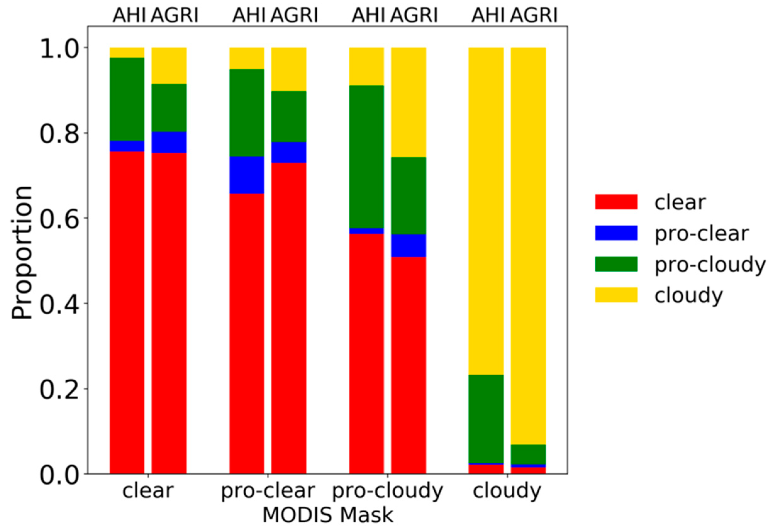
| Cloud Mask | Cloud Phase | ||||||
|---|---|---|---|---|---|---|---|
| clear | pro-clear | pro-cloudy | cloudy | Water | Mixed | Ice | |
| MODIS | 22% | 4% | 15% | 59% | 52% | 1% | 47% |
| AHI | 22% | 1% | 29% | 48% | 52% | 7% | 41% |
| AGRI | 23% | 2% | 14% | 61% | 53% | 4% | 43% |
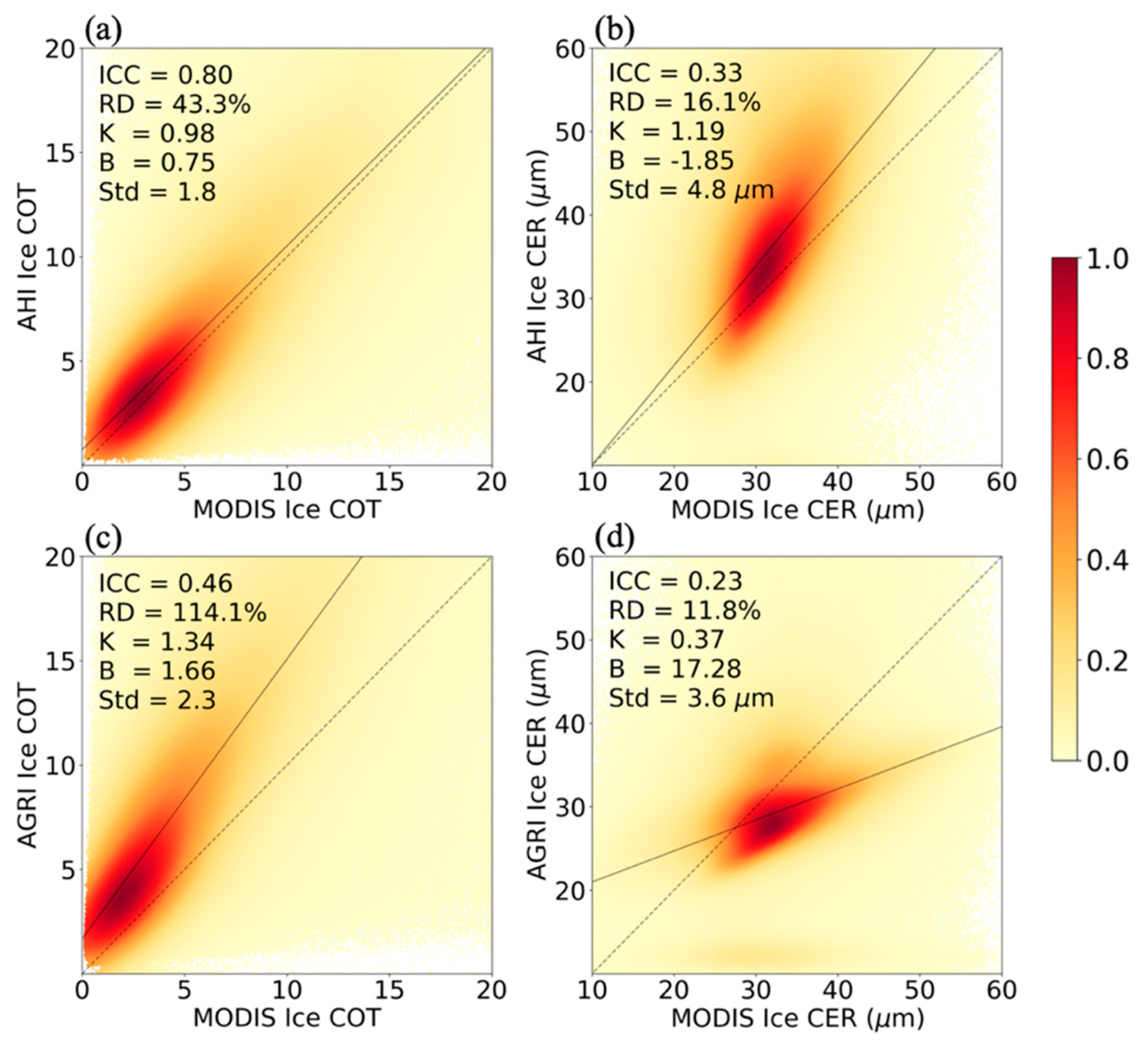
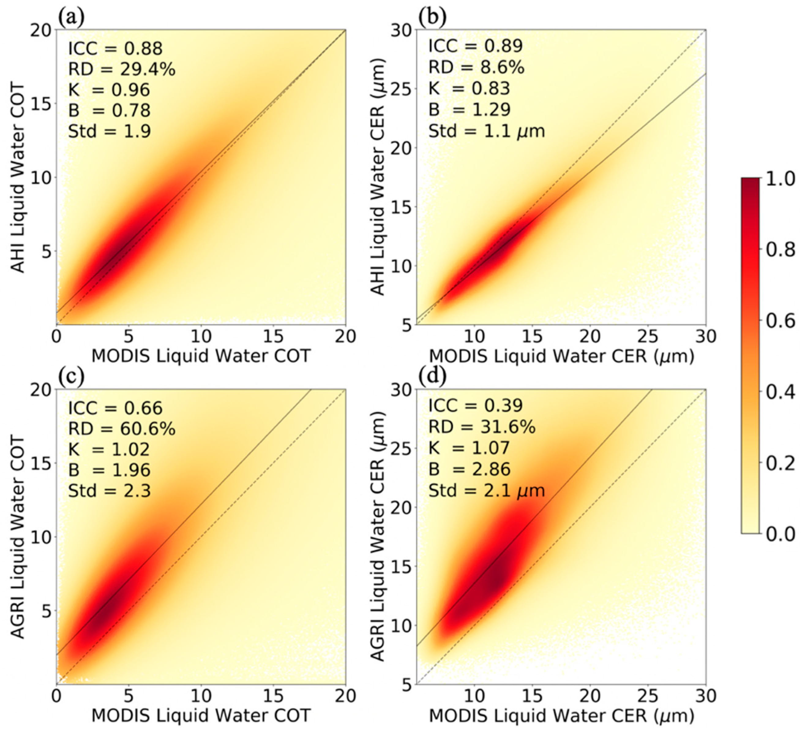
| AHI | AGRI | ||||||||||
|---|---|---|---|---|---|---|---|---|---|---|---|
| K | B | ICC | RD | Std | K | B | ICC | RD | Std | ||
| Ice | COT | 0.98 | 0.75 | 0.80 | 43.3% | 1.8 | 1.34 | 1.66 | 0.46 | 114.1% | 2.3 |
| CER | 1.19 | −1.85 | 0.33 | 16.1% | 4.8 | 0.37 | 17.28 | 0.23 | 11.8% | 3.6 | |
| Water | COT | 0.96 | 0.78 | 0.88 | 29.4% | 1.9 | 1.02 | 1.96 | 0.66 | 60.6% | 2.3 |
| CER | 0.83 | 1.29 | 0.89 | 8.6% | 1.1 | 1.07 | 2.86 | 0.39 | 31.6% | 2.1 | |
| VZA | 0–10° | 10–20° | 20–30° | 30–40° | 40–50° | 50–60° | 60–70° |
|---|---|---|---|---|---|---|---|
| τAHI | 7.9 | 9.4 | 9.1 | 13.6 | 11.0 | 11.2 | 12.1 |
| τAGRI | 8.5 | 10.8 | 8.8 | 9.2 | 12.9 | 20.6 | 28.3 |
| RD (AHI-MODIS) | 38% | 37% | 28% | 27% | 19% | 18% | 21% |
| RD (AGRI-MODIS) | 28% | 34% | 44% | 43% | 62% | 115% | 152% |
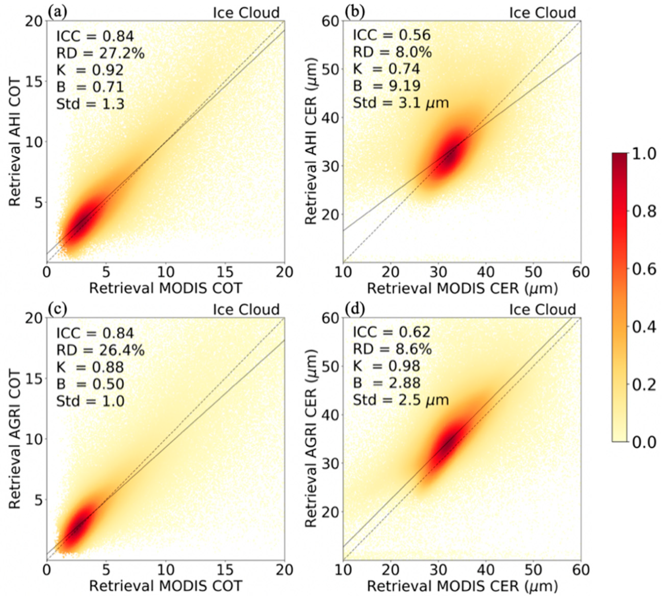
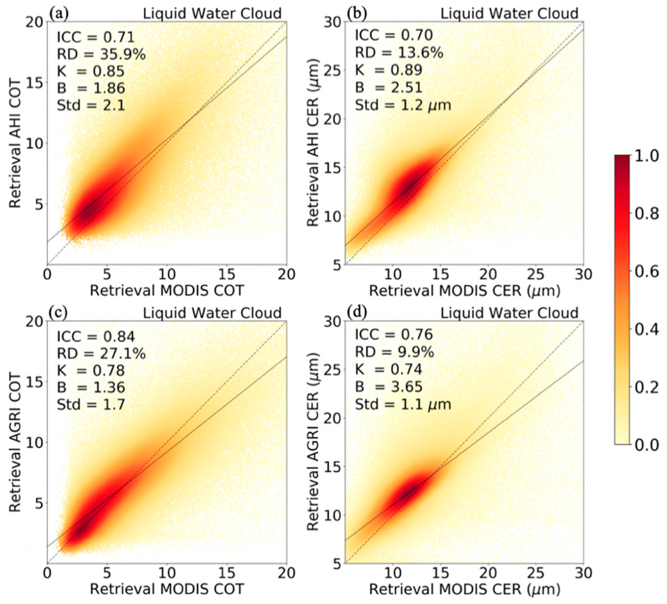
| AHI | AGRI | ||||||||||
|---|---|---|---|---|---|---|---|---|---|---|---|
| K | B | ICC | RD | Std | K | B | ICC | RD | Std | ||
| Ice | COT | 0.92 | 0.71 | 0.84 | 27.2% | 1.3 | 0.88 | 0.50 | 0.84 | 26.4% | 1.0 |
| CER | 0.74 | 9.19 | 0.56 | 8.0% | 3.1 | 0.98 | 2.88 | 0.62 | 8.6% | 2.5 | |
| Water | COT | 0.85 | 1.86 | 0.71 | 35.9% | 2.1 | 0.78 | 1.36 | 0.84 | 27.1% | 1.7 |
| CER | 0.89 | 2.51 | 0.70 | 13.6% | 1.2 | 0.74 | 3.65 | 0.76 | 9.9% | 1.1 | |
© 2019 by the authors. Licensee MDPI, Basel, Switzerland. This article is an open access article distributed under the terms and conditions of the Creative Commons Attribution (CC BY) license (http://creativecommons.org/licenses/by/4.0/).
Share and Cite
Lai, R.; Teng, S.; Yi, B.; Letu, H.; Min, M.; Tang, S.; Liu, C. Comparison of Cloud Properties from Himawari-8 and FengYun-4A Geostationary Satellite Radiometers with MODIS Cloud Retrievals. Remote Sens. 2019, 11, 1703. https://doi.org/10.3390/rs11141703
Lai R, Teng S, Yi B, Letu H, Min M, Tang S, Liu C. Comparison of Cloud Properties from Himawari-8 and FengYun-4A Geostationary Satellite Radiometers with MODIS Cloud Retrievals. Remote Sensing. 2019; 11(14):1703. https://doi.org/10.3390/rs11141703
Chicago/Turabian StyleLai, Ruize, Shiwen Teng, Bingqi Yi, Husi Letu, Min Min, Shihao Tang, and Chao Liu. 2019. "Comparison of Cloud Properties from Himawari-8 and FengYun-4A Geostationary Satellite Radiometers with MODIS Cloud Retrievals" Remote Sensing 11, no. 14: 1703. https://doi.org/10.3390/rs11141703
APA StyleLai, R., Teng, S., Yi, B., Letu, H., Min, M., Tang, S., & Liu, C. (2019). Comparison of Cloud Properties from Himawari-8 and FengYun-4A Geostationary Satellite Radiometers with MODIS Cloud Retrievals. Remote Sensing, 11(14), 1703. https://doi.org/10.3390/rs11141703