Abstract
The objective of this paper was to evaluate the use of in situ normalized difference vegetation index (NDVIis) and Moderate Resolution Imaging Spectroradiometer NDVI (NDVIMD) time series data as proxies for ecosystem gross primary productivity (GPP) to improve GPP upscaling. We used GPP flux data from 21 global FLUXNET sites across main global biomes (forest, grassland, and cropland) and derived MODIS NDVI at contrasting spatial resolutions (between 0.5 × 0.5 km and 3.5 × 3.5 km) centered at flux tower location. The goodness of the relationship between NDVIis and NDVIMD varied across biomes, sites, and MODIS spatial resolutions. We found a strong relationship with a low variability across sites and within year variability in deciduous broadleaf forests and a poor correlation in evergreen forests. Best performances were obtained for the highest spatial resolution at 0.5 × 0.5 km). Both NDVIis and NDVIMD elicited roughly three weeks later the starting of the growing season compared to GPP data. Our results confirm that to improve the accuracy of upscaling in situ data of site GPP seasonal responses, in situ radiation measurement biomes should use larger field of view to sense an area, or more sensors should be placed in the flux footprint area to allow optimal match with satellite sensor pixel size.
1. Introduction
The normalized difference vegetation index (NDVI [1]) is a well-recognized proxy of canopy greenness [2,3,4] that relates to ecosystem photosynthetic carbon uptake. NDVI is widely used in ecosystem modelling studies because interannual and intra-seasonal dynamics of gross primary productivity (GPP) are driven by changes in ecosystem phenology that directly affect total annual ecosystem carbon budgets [5,6,7,8]. Even though new vegetation remotely based indices have been proposed for the estimation of ecosystem productivity (i.e., enhanced vegetation index (EVI) [3], photochemical reflectance index (PRI) [9], and chlorophyll content index (CCI) [10]), NDVI is extensively employed in ecological models and landscape mapping due to its long record available from Advanced Very-High-Resolution Radiometer (AVHRR) sensors [11,12,13,14].
A number of studies have analyzed the impact of climate change on GPP and ecosystem greenness phenology. Changes in ecosystem greenness have generally been described at local and regional scales using in situ observations provided by eddy covariance flux data of carbon dioxide exchange, webcams, and satellite data [15,16,17,18,19,20,21]. Global scale land surface models are parameterized using earth observation data, where the NDVI is widely used as an indicator of ecosystem greenness [22,23] due to its linking of photosynthesis with carbon uptake in main terrestrial ecosystems [24,25,26,27,28]. A range of satellite products (MODIS/Terra or MODIS/Aqua, https://modis.gsfc.nasa.gov/; SPOT/VGT, http://www.spot-vegetation.com/; and NOAA/AVHRR, https://www.ncdc.noaa.gov/) have been studied to increase understanding of changes in ecosystem greenness at the global scale; however, impacts of landscape heterogeneity and spatial scale on the relationship between greenness and ecosystem productivity are unclear [29,30] because research tends to be based on local scale, single-site studies. Field-based measurements of the NDVI are time consuming, particularly in highly heterogeneous landscapes, and field sampling protocols tend to be based on the Validation of European Remote Sensing Instruments (VALERI [31], http://w3.avignon.inra.fr/valeri/) protocol for the estimation of NDVI, leaf area index (LAI), or vegetation cover. The VALERI method was developed for various spatial scales, from small study plots to the size of a pixel, of coarse-resolution satellite data. The VALERI database is available on request for a large number of sites worldwide at the http://w3.avignon.inra.fr/valeri/fic_htm/database/main.php webpage. Geostatistical techniques and pixel-based classification algorithms offer a valuable alternative for an accurate and precise classification of landscape [32,33]. GPP and NDVI field measurements are scaled up using in situ FLUXNET [34] radiation data [35,36], and subsequent regression analysis is often used to define transfer functions that allow the estimation of GPP from NDVI data. However, the uncertainties related to the scale mismatch between the in situ point measurements, flux footprint, and the pixel resolution remain a critical issue.
Thus, investigation of the relationship between seasonal NDVI dynamics and GPP requires quantitative estimation of landscape heterogeneity to improve the estimation of plant functional type (PFT) changes in GPP, and we consider landscape spatial heterogeneity versus homogeneity to be essential in inter-site comparisons of flux, particularly when remotely sensed data are derived from contrasting spatial resolutions. Here, our aim was to evaluate up-scaled in situ and time series data as proxies for ecosystem and landscape-scale GPP. The specific objectives were to:
- (i)
- Describe in situ NDVI (NDVIis) seasonal dynamics using Fourier time series modeling and analysis;
- (ii)
- Compare multi-temporal NDVIis time series dynamics derived from radiation measurements using Moderate Resolution Imaging Spectroradiometer (MODIS) NDVI data (NDVIMD) computed for contrasting spatial scales and biomes;
- (iii)
- Quantify landscape heterogeneity from flux tower footprints;
- (iv)
- Use these approaches to model GPP seasonal dynamics.
2. Materials and Methods
2.1. Derivation of NDVIis from In Situ Radiation Measurements
In situ radiometric data were selected from FLUXNET eddy covariance databases (www.fluxdata.org), where particular use was made of a subset of open and fair-use data in the La Thuile database. From these, we selected 21 flux sites that represented a global spatial distribution and had high quality and continuous data for the calculation of NDVIis (Table S1). We defined and computed NDVIisbased on half-hourly in situ measurements of incoming and outgoing photosynthetically active radiation ( and , respectively) and global incoming and outgoing shortwave radiation ( and , respectively), as proposed by Huemmrich et al. [37]. Reflectance (ρ) in the PAR region (ρPAR, spectral range 400–700 nm) and reflectance in the NIR region (ρNIR, spectral range 700–2800 nm) were calculated as:
where and are expressed in J·m−2·s−1, using a conversion factor of 4.55 μmol·J−1 from μmol·photons·m−2·s−1 [38]. and are expressed in J·m−2·s−1.
In situ ρPAR and ρNIR reflectances were then used to compute in situ NDVI [39], as defined by Equation (3):
Typically, at FLUXNET sites, and are measured by coupling two quantum sensors— is measured by an upward-faced quantum sensor while by a downward-facing sensor. and are measured by two pyranometers—one faces upward to measure and the other faces downward to measure [40]. Both instruments are affected by very low uncertainty that is around 2% of and spans from 2% to 3% for . Therefore, the uncertainty of radiation measurements is treasurable in NDVIis estimation. The quality of half-hourly radiometric measurements was checked by applying different physical tests (e.g., has to be less than the corresponding extraterrestrial radiation at the same point of time) and by the analysis of the statistical variability of the data (quantified by the standard deviation), as proposed in [35].
Daily NDVIistime series were computed from the average of five half-hourly radiation data points recorded over the period 11:00 to 13:00 local solar time that corresponded with the overpassing of the MODIS/TERRA satellite.
2.2. MODIS Data and Processing
We used the 8 day, 500 m surface reflectance product (MOD09G1, collection 5) from the MODIS/TERRA satellite provided by ORNL-DAAC (http://daac.ornl.gov/cgi-bin/MODIS/GR_col5_1/mod_viz.html) for the 21 sites to compute MODIS NDVI (NDVIMD), from which a time series was calculated, with spatial pixel aggregations comprising:
- (i)
- A single pixel with coordinates matching a flux site (MODIS0.5×0.5: 0.5 × 0.5 km);
- (ii)
- Nine pixels centered around a flux site (MODIS1.5×1.5: 1.5 × 1.5 km);
- (iii)
- Twenty-five pixels centered around a flux site (MODIS2.5×2.5: 2.5 × 2.5 km);
- (iv)
- Forty-nine pixels centered around a flux site (MODIS3.5×3.5: 3.5 × 3.5 km).
The MOD09G1 product includes optimal reflectance values for nine bands in the visible and NIR regions, and the 8-day compositing period uses highest quality pixels (clear sky conditions and no snow cover) selected with optimal viewing angles and minimal cloud or cloud shadow impacts that were retained for further processing. NDVIMD for the aggregation of pixels ≥0.5 km (MODIS1.5×1.5, MODIS2.5×2.5 and MODIS3.5×3.5) was calculated as:
where ρred and ρNIR are the reflectance values for MODIS band 1 (620–670 nm) and band 2 (841–871 nm), respectively.
NDVIMD = (ρNIR − ρred)/(ρNIR + ρred)
We used the MOD13Q1 NDVI dataset with 250 m pixel size and a 16 day compositing period to quantify landscape spatial variability in the area surrounding an eddy covariance tower because this product has an increased spatial resolution of 250 m compared to MOD09 (500 m). The best image at the beginning of the season, which was as close as possible to the starting day of greening, was selected for each site (Table S1). Pixels corresponding to an area of 7 × 7 km were extracted, then the extracted area was classified, and the spatial heterogeneity indicator (SHI) was computed (determination methodology for SHI is described in Section 2.4). MODIS data quality was assured by making use of the quality assurance and control (QA/QC) flags available in MOD09G1.
2.3. NDVI Time Series Analysis: Fourier Modeling and Fitting
To compare NDVIis with NDVIMD data at an 8-day time resolution, 8-day NDVIis time series were derived from daily in situ NDVIis time series, where days corresponding with the optimal MOD09G1 data were extracted and modeled using Fourier time series software in FORTRAN 77 (see Figure 1 for an example).
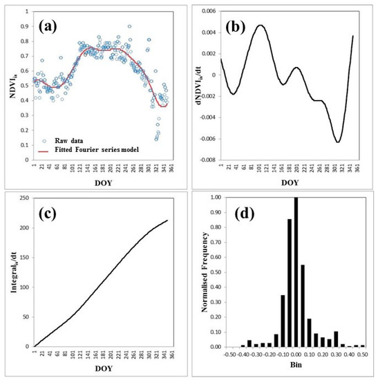
Figure 1.
Example of output from an in situ normalized difference vegetation index (NDVIis) Fourier time series (Equation (5)) for a deciduous forest site (Missouri Ozark site, USA). (a) NDVIis data (blue circles) and NDVIis fit (red line), (b) first derivative of the NDVIistime series, (c) integral over one year of the NDVIis time series, and (d) histogram of the normalized residuals of the NDVIis fit of NDVIis time series data points.
A Fourier series expansion equation was used as a data fitting model for the NDVIis and NDVIMD 1 year time series to allow formalization of seasonal dynamics, where optimal fit was obtained when the root mean square error (RMSE) for the number of harmonics used in the model was minimal. The Fourier series expansion was defined as:
with
and
The first derivative and integral over the NDVI time series, which were obtained using Equations (8) and (9), represent the analytical expression in Equation (5).
where a0, a1, a2 are the Fourier series coefficients; L is the number of Fourier series harmonics; t is time (Day Of Year, DOY); and n is the number of Fourier terms.
The use of five harmonics led to a Gaussian frequency distribution of residuals, where the standard deviation (SD) is at its minimum with extreme number of harmonics (L). In the optimization of fit, SDs were determined by fitting a normalized Gaussian model to the normalized frequency distribution of residuals (Figure 1d).
2.4. Development of a Spatial Heterogeneity Indicator (SHI) for Categorical Maps
Landscape spatial heterogeneity versus homogeneity is essential in the comparison of site differences in flux, particularly at contrasting spatial resolutions. Site homogeneity/heterogeneity is quantified by defining a quantitative spatial heterogeneity indicator (SHI). Here the SHI is based on categorical classified imagery and quantifies the degree of biome spatial heterogeneity. The determination of the SHI is inspired by a landscape ecology approach; therefore, spatial variability in vegetation surrounding a flux tower was determined by integrating information retrieved from a MOD13Q1 image classification using a decision tree classification (DTC) (described in Section 2.5). Imagery was selected for each of the 21 flux sites from MOD13Q1 NDVI data at a 250 m pixel size and a 16 day compositing period with QA/QC checks performed. We selected the best image at the beginning of the season, as close as possible to the start day of greening (for more details, see Table S1).
2.5. Decision Tree Classification
A DTC is a systematic land use classification approach to producing categorical maps, based on specific (mostly bio-geophysical) input data sets, where techniques, such as DTC classifiers, rule-based classifiers, neural networks, support vector machines, and naive Bayes classifiers, are used to solve an image or land use classification problem. Each technique starts with a learning algorithm to define a model that best fits the relationship between the attribute set and class labels of input data. Therefore, a key objective of the learning algorithm is to build a predictive model that accurately predicts the class labels of records belonging to a previously unknown class.
DTC classifier is a simple and widely used classification technique that consists of an iterative series of criteria and conditions in a decision tree, based on the bio-geophysical attributes of a pixel that ultimately leads to the classification of the pixel. In the DTC decision tree, the root and internal nodes contain the attribute test conditions that separate data records with contrasting characteristics. A class label, which accepts the values “Yes” or “No”, is assigned at the terminal node, resulting in a categorical pixel classification map. The description of the criteria used to classify NDVI pixels by using DTC classifier are reported in Table 1.

Table 1.
Description of the criteria to classify NDVI pixels by using decision tree classification (DTC) classifier.
The categorical pixel classification map originated from DTC classification method and for each flux site were used to calculate SHI for each site as described in Section 2.6.
2.6. Quantification of Biome Spatial Heterogeneity Based on a Categorical Map
Spatial heterogeneity is generally defined as the spatial complexity and variability of a landscape property (a biome), and despite its importance in many applications, including in landscape ecology, a formal and rigorous definition remains lacking [41]. Nonetheless, an operational definition is required to facilitate quantitative evaluations, so we defined an SHI based on the categorical classification, as described here below (Figure 2 and Table 2).
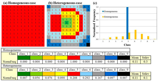
Figure 2.
Categorical arrays for a homogeneous (a) and heterogeneous (b) landscape. (c) Normalized frequency distributions for the homogeneous and heterogeneous arrays of pixels. The table shows the classes and corresponding normalized frequencies (NormFreq) for the nine classes in the pixel array of the homogeneous and heterogeneous landscapes (Stdev: Standard deviation).
Table 2.
Sum (SUM), sum squared (SSQ), kurtosis and spatial heterogeneity index (SHI) for the categorical arrays of the homogeneous and heterogeneous landscapes in Figure 2.
2.7. Comparison of NDVIis and NDVIMD
We analyzed effects of spatial scale on the relationships between NDVIis and NDVIMD with biome properties, using coefficient of determination (CORR), root mean square error (RMSE), and mean absolute percentage error (MAPE/75) statistics, by re-grouping selected flux sites according to the biome to which they belong.
2.8. Flux Data and GPP Estimation
For the selected sites reported in Table S1, we gathered half-hourly CO2 fluxes from the FLUXNET eddy covariance “La Thuile” database (www.fluxdata.org). These data were quality flagged for sensor malfunctions or not ideal turbulence conditions [42] and gap-filled following the marginal distribution sapling method [43].
GPP was estimated using flux partitioning, based on the extrapolation of nighttime flux observations corrected for temperature differences with temperature-dependency relationships [43]. Finally, we calculated GPP daily means from the half-hourly data over the period corresponding with the MODIS/TERRA satellite overpass and corresponding with the time interval used for radiation measurements to calculated in situ NDVIis (from 11:00 to 13:00 local solar time; for more details see Section 2.1).
To compare the start of the season (SOS) of GPP with SOS NDVIis and SOS NDVIMD, 8-day GPP time series were derived from daily in situ GPP time series and modeled using Fourier time series analysis as applied for NDVIis (Section 2.3).
3. Results
3.1. Relationship Between NDVIis and NDVIMD across and within Biomes
In general, the relationship between NDVIis and NDVIMD varied across the biomes and within biomes with spatial resolution (Table 3, Figure S1). Overall, the strongest correlation was obtained for deciduous broadleaf forests (DBF) (CORR = 0.70, RMSE = 0.10, p < 0.001) (Table 3). Strength of relationship was consistently high in open shrubland (OSH) sites as well (CORR = 0.68, RMSE = 0.10, p < 0.001), as elicited for DBF. In addition, the relationship between NDVIis and NDVIMD presented the same slope of 0.90, indicating that NDVIis was slightly lower than NDVIMD for both biomes. Moderately strong relationships were recorded in woody savannas (WSA: CORR = 0.54, RMSE = 0.04, p < 0.001) and croplands (CRO: CORR = 0.53, RMSE = 0.20, p < 0.001). However, these last two biomes showed a very different slope of the relationship between NDVIis and NDVIMD (CRO: Slope = 0.93; WSA: Slope = 0.40) showing a quite large disagreement between NDVIis and NDVIMD for WSA biome. Relationships were consistently low at all spatial resolutions in grasslands, evergreen needleleaf (ENF), and broadleaf (EBF) (Table 3). The best CORR values were found at the highest spatial resolution (0.5 × 0.5 km) for all biomes, except for OSH that was at lowest spatial resolution (3.5 × 3.5 km) and for EBF that was at 1.5 × 1.5 km. Nevertheless, the goodness of relationship slightly (±3%) varied within the same biome (Table 3). EBF exhibited the lowed variability (±3%) while ENF exhibited the highest (±7%).
Table 3.
Results of the regression analysis of the relationship between NDVIis and NDVIMD at different spatial resolutions (0.5 × 0.5 km; 1.5 × 1.5 km; 2.5 × 2.5 km; 3.5 × 3.5 km) among biomes. CRO: Cropland; DBF: Deciduous broadleaf forest; EBF: Evergreen broadleaf forest; ENF: Evergreen needle leaf forest; GRA: Grassland; OSH: Open shrubland; and WSA: Woody savanna. The table underneath the figure shows statistical metrics: CORR: Correlation of determination; * p < 0.001; number of available days; RMSE: Root mean square error; MAPE/75: Mean absolute percentage error/75; slope: Slope of the linear model; Y-int: y-intercept of the linear model.
The distribution of the CORR values across biomes on a site × year basis showed a much-reduced variability for all OSH (Figure S1). WSA and EBF sites also showed a reduced variability (Figure S1). DBF and GRA biomes showed a quite marked variability and CRO a very large variability that can be related to the specific year-to-year site management as crop rotation (Figure S1).
3.2. Site Level Variation in Relationship Between NDVIis and NDVIMD
Analysis of the distribution of CORR values for sites grouped by biomes showed a low variability within DBF, EBF, and WSA sites (Figure 3b,c,g). DBF sites had largest CORR values with a limited variability across sites and spatial resolutions and within sites-years, except for US-MOz site where a good relationship was found only at 0.5 × 0.5 km spatial resolution. WSA site showed comparable low variability within years and across spatial resolutions. CORR values of EBF site were very low with years and across the spatial resolutions. A very low variability was found at highest spatial resolution (Figure 3c). Strength of relationships were variable within years and across sites for CRO, ENF, and GRA. CRO and GRA sites tended to have a highest CORR at the highest spatial resolution. For CRO on average, the CORR values of DE-Geb were highest at the 0.5 × 0.5 km spatial resolution compared with other sites within the respective biome, while US-ARM site showed very poor correlation. There was greater within-years variability in relationships in the US-FPe and US_Goo grassland sites. Relationships were generally weak in the ENF sites, with the exception of CA-NS5. There were a large within-year variability in relationships for OSH sites.
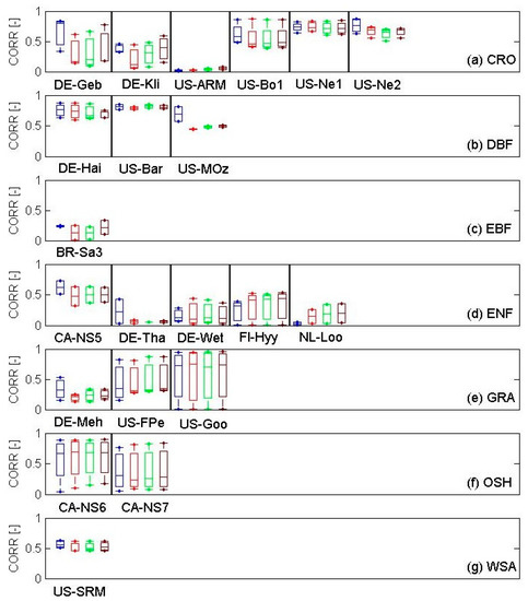
Figure 3.
Analysis of relationship (CORR: Coefficient of determination) between NDVIis and NDVIMD at different spatial resolutions (0.5 × 0.5 km: blue; 1.5 × 1.5 km: red; 2.5 × 2.5 km: green; and 3.5 × 3.5 km: brown) in different biomes (a) CRO: Cropland; (b) DBF: Deciduous broadleaf forest; (c) EBF: Evergreen broadleaf forest; (d) ENF: Evergreen needle leaf forest; (e) GRA: Grassland; (f) OSH: Open shrubland; and (g) WSA: Woody savanna).
3.3. Site Level Seasonal Variability
Fourier series modeling of NDVIisat eddy covariance tower sites in different biomes showed greatest seasonal amplitude for the first derivative in CRO, DBF, and OSH (Table 4) and large seasonality in the fitted NDVIis time series in DBF and CRO (Figure 4a,b, respectively). The seasonality of these biomes was well represented by NDVIMD too. Although there were large seasonal amplitudes for the first derivative in grasslands, there were high levels of between-site variation. Lowest levels of seasonal amplitude for the first derivative and fitted time series were recorded from ENF and woody savanna (Figure 4c,d).
Table 4.
Fourier modeling of NDVIis time series data on a site × year basis. PFT: Plant functional type; CRO: Cropland; DBF: Deciduous broadleaf forest; EBF: Evergreen broadleaf forest; ENF: Evergreen needle leaf forest; GRA: Grassland; OSH: Open shrubland; and WSA: Woody savanna. Average*1000: Average of first derivative of the NDVIis time series; Stdev: Standard deviation of first derivative of the NDVIis time series; Max: Maximum of the first derivative of the NDVIis; Min: Minimum of the first derivative of the NDVIis; Amplitude: Difference between Max and Min of the first derivative of the NDVIis.
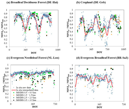
Figure 4.
Example output of in situ Fourier series model fitted to NDVI (NDVIis) time series data of: (a) a deciduous broadleaf forest (BDF); (b) a cropland (CRO); (c) an evergreen needle leaf forest (ENF); and (d) an evergreen broadleaf forest (EBF). Blue circles represent raw NDVIis data and red lines represent Fourier series fitted NDVIis data. Filled dots represent MODIS NDVI time series at different spatial resolutions (0.5 × 0.5 km: Green; 1.5 × 1.5 km: Orange; 2.5 × 2.5 km: Dark green; and 3.5 × 3.5 km: Black).
3.4. Site Heterogeneity Index Application
Overall, we found the SHI for all DBF and ENF sites and for WSA sites (US-SRM) and the two OSH sites were zero, indicating site homogeneity. SHI at the other sites was >0, indicating site heterogeneity (Table 5). SHI was particularly high at the US-Ne1 and US-Ne2 crop sites. This could be related to the fact that the SHI was developed over an area of 7 × 7 km, not considering the different crop parcels in this area.
Table 5.
Spatial heterogeneity index (SHI) for different flux sites. Letters in bold indicate SHI for heterogeneous sites.
3.5. GPP Seasonality
Overall, both NDVIis and NDVIMD tended to predict the start of the growing season about three weeks later than the start of season derived from GPP data (Figure 5, Table 6). However, the prediction of the start of season of GPP using NDVIis was more accurate than NDVIMD at 0.5 × 0.5 km (R2 = 0.53; R2 = 0.34, respectively), and NDVIis predicted the start of season of GPP roughly one week before (RMSE = 27.78 days) NDVIMD(RMSE = 32.90 days) (Table 6). The estimation of the start of the growing season of GPP was high variable across biomes for both NDVIisand NDVIMD, which showed limitations mainly for WSA and EBF sites (Figure 5).
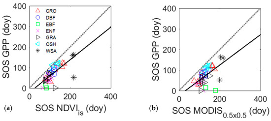
Figure 5.
Relationship between the start of season (SOS) derived from GPP eddy covariance data (in days) for different biomes and data derived from (a) NDVIis and (b) NDVIMD at a spatial resolution of 0.5 × 0.5 km. ENF: Evergreen needle leaf forest; EBF: Evergreen broadleaf forest; DBF: Deciduous broadleaf forest; GRA: Grassland; CRO: Cropland; WSA: Woody Savanna; and OSH: Open shrubland.
Table 6.
Relationship between the start of season (SOS) of GPP derived from eddy covariance data (days) and the start of greenness derived from NDVIis and NDVIMD at a spatial resolution of 0.5 × 0.5 km. Observations: Number of available days; R2: Root mean square error; RMSE: Root mean square error; NMB: Normalized mean bias; Slope: Slope of the linear model; Y-int: y-intercept of the linear model; R2cv: Cross-validated coefficient of determination.
4. Discussion
4.1. Trees Density and Spatial Distribution, and Management
An important finding from our analysis was the variation in relationship between NDVIis and NDVIMD across biomes and sites (Figure 3). The strong relationship, which was characterized by low variability, in DBF (Figure 3b) may be explained by the strong seasonal dynamics in the biome (Figure 4a) and high levels of site spatial homogeneity (Table 5). The good performance of the relationship in open shrubland (OSH) can be related to the species composition of this biome that is generally characterized by two different type of vegetation: Evergreen or deciduous shrubland and natural grass that can have a very different phenology. The density and the spatial distribution of shrubs could explain the high variability in the performances. Similar to OSH, the distribution and density of trees play a relevant role in the goodness of the relationships for the woody savannas (WSA) biome. The high variability in the NDVIis–NDVIMD relationship for grasslands and croplands may be related to site heterogeneity (Table 5) and site management (i.e., rotation with different crops, manures, irrigation, harvest) of crops and grasses in the area of 7 × 7 km considered for SHI calculations. Generally, crop fields are monoculture, but they can have a much-reduced extent, and the crop type and phenology can change from one field to the next (i.e., crop rotations). Grasslands can be natural or managed by harvesting or livestock in the same area. Therefore, the spatial distribution of grasslands and croplands vegetation components, such as crop density, litter, and species composition, and canopy structure characteristics, such as the presence of an understory with a contrasting NDVI phenology, are key factors in the determination of the start of the greening and carbon uptake seasons. We found that specific year-to-year site management tended not to be accounted for in data upscaling, particularly for sites with a single crop (US-Ne1) or under crop rotation (US-Ne2) and grazed and harvested grassland sites (DE-Meh). The poor performance in the relationships of evergreen forest (ENF and EBF) is possibly due to the low seasonal variability, as indicated by low NDVI seasonal amplitude (Figure 4), particularly in ENF that were classified by the SHI as spatially homogenous (Table 5).
4.2. NDVI Seasonal Variability and GPP Seasonality
These results support previous studies of deciduous forest biomes, which are typified by a strong dependence of photosynthetic activity on leaf area expansion, that showed MODIS and in situ NDVI data patterns correspond with dynamics of net ecosystem exchange [35] and GPP [19,44]. Furthermore, the production and the expansion of the new leaves in spring needed for activating the photosynthetic process provoke an evident spectral shift that has a clear effect on canopy greenness [16,19]. For that reason, the start of growing seasons of DBF can be estimated by remotely sensed indicators of the canopy greenness [17,45].
In contrast, we found a weak relationship between the two NDVIs in evergreen forests. However, our results agree with previous studies where the start of season of DBF is more successfully detected than for evergreen needleleaf and broadleaf biomes [44]. In fact, in evergreen biomes, the expansion of leaves is unrelated to the start of spring photosynthetic activity and GPP and uncoupled with changes in spring greenness [46]. In addition, in boreal evergreen biomes, the annual phenological cycles are related more to snow and snow melt than changes in needle canopy greening dynamics in boreal climates, as shown in the work of Jönsson et al. [47]. Given that the change in greenness of ENF at the start of the growing season may be decoupled from the start of seasonal carbon uptake, and hence may be independent of ecosystem physiological activity [48], and the view that NDVI may not be an effective proxy for the estimation of seasonal changes in GPP phenology [17], the chlorophyll content index (CCI; [10]) has been proposed as a more accurate remote sensing based proxy to estimate GPP phenology and seasonal dynamics in ENF [27].
4.3. Spatial Resolution and Sensors Characteristics
We generally found that the strength of the NDVIis–NDVIMD relationship tended to decrease with decreasing spatial resolution (from 0.5 × 0.5 to 3.5 × 3.5 km, Figure 3), this is due to a closer spatial correlation between the NDVIis and NDVIMD 0.5km product as a consequence of the limited spatial representation for the in situ NDVI. In situ radiation sensors are generally mounted a few meters above the canopy, limiting radiation measurements to a small area that is not representative of the biome or landscape. This is particularly true in heterogeneous sites [35], while the instant field of view (IFOV) of the radiometric measurements tends to be too small to effectively represent a landscape or plant functional type [36,40]. The potential use of in situ radiation measurement data in the upscaling of site responses may be improved by increasing the spatial representativeness of the canopy dynamics. For example, the radiometer should be placed at the convenient distance above the canopy to sense a larger area that is comparable at the satellite pixels. To reduce the mismatch between in situ and satellite measurements, it could be helpful to have more than one radiation sensor for at least downward radiation measurements in the flux footprint area (i.e., a mobile track or transect). This allows to better identify the in situ spatial variability of canopy reflectance. A precise estimation of the flux footprint could also help to improve the upscaling of in situ data. Flux footprint is assumed to vary between 10 to 100 times of the measurements height; however, this assumption tends to overestimate the flux source area [49]. The recent launch of the space borne high-resolution ESA Sentinel-2 mission (10 m × 10 m) opens a unique opportunity in phenological application and upscaling flux and in situ data.
5. Conclusions
We found limitations of MODIS and in situ NDVI in the capture of GPP seasonal dynamics for evergreen forests due to insufficient description of plant ecophysiology by the NDVIs, and landscape heterogeneity estimated using the SHI of PFT is essential in upscaling GPP data.
Our results confirm that to improve the accuracy of upscaling in situ data of site GPP seasonal responses, in situ radiation measurements should use larger field of view to sense an area or more sensors should be placed in the flux footprint area allow optimal match with satellite sensor pixel size.
Supplementary Materials
The following are available online at https://www.mdpi.com/2072-4292/11/14/1656/s1, Figure S1: Results of the statistical analysis between NDVIis and NDVIMD for different spatial resolutions, Table S1: Description of FLUXNET sites used in this study.
Author Contributions
Conceptualization, M.B.; methodology, M.B. and F.V.; formal analysis, M.B.; writing—original draft preparation, M.B.; writing—review and editing, all co-authors.
Funding
This project received funding from the European Union Horizon 2020 Research and Innovation program under the Marie Skłodowska-Curie grant (INDRO, grant no 702717).
Acknowledgments
This work used radiometric and eddy covariance measurements acquired by the FLUXNET community, in particular by AmeriFlux (US Department of Energy, Biological and Environmental Research, Terrestrial Carbon Program (DE-FG02-04ER63917 and DE-FG02-04ER63911)), AfriFlux, AsiaFlux, CarboAfrica, CarboEuropeIP, CarboItaly, CarboMont, ChinaFlux, FLUXNET—Canada (supported by CFCAS, NSERC, BIOCAP, Environment Canada, and NRCan), GreenGrass, KoFlux, LBA, NECC, OzFlux, TCOS—Siberia, and USCCC. We acknowledge the support to data harmonization provided by CarboEuropeIP, FAO-GTOS-TCO, iLEAPS (the Integrated Land Ecosystem-Atmosphere Processes Study, a core project of IGBP), Max Planck Institute for Biogeochemistry, National Science Foundation, University of Tuscia, Université de Laval, Environment Canada, US Department of Energy, and database development and technical support from Berkeley Water Center, Lawrence Berkeley National Laboratory, Microsoft Research eScience, Oak Ridge National Laboratory, University of California—Berkeley, and University of Virginia. The authors acknowledge support of the PIs of the eddy covariance sites and technicians, under- and post-graduate students and post-doctoral researchers for providing data and support to the FLUXNET network. The MODIS data used in this study are distributed by the Land Processes Distributed Active Archive Center (LP DAAC), located at the US Geological Survey (USGS) Earth Resources Observation and Science (EROS) Center (lpdaac.usgs.gov).
Conflicts of Interest
The authors declare no conflict of interest.
References
- Tucker, C.J. Red and photographic infrared linear combinations for monitoring vegetation. Remote Sens. Environ. 1979, 8, 127–150. [Google Scholar] [CrossRef]
- Reed, B.C.; Brown, J.F.; VanderZee, D.; Loveland, T.R.; Merchant, J.W.; Ohlen, D.O. Measuring phenological variability from satellite imagery. J. Veg. Sci. 1994, 5, 703–714. [Google Scholar] [CrossRef]
- Huete, A.; Didan, K.; Miura, T.; Rodriguez, E.P.; Gao, X.; Ferreira, L.G. Overview of the radiometric and biophysical performance of the modis vegetation indices. Remote Sens. Environ. 2002, 83, 195–213. [Google Scholar] [CrossRef]
- Piao, S.; Fang, J.; Zhou, L.; Ciais, P.; Zhu, B. Variations in satellite-derived phenology in China’s temperate vegetation. Glob. Chang. Biol. 2006, 12, 672–685. [Google Scholar] [CrossRef]
- Richardson, A.D.; Black, T.A.; Ciais, P.; Delbart, N.; Friedl, M.A.; Gobron, N.; Hollinger, D.Y.; Kutsch, W.L.; Longdoz, B.; Luyssaert, S.; et al. Influence of spring and autumn phenological transitions on forest ecosystem productivity. Philos. Trans. R. Soc. Lond. Ser. B Biol. Sci. 2010, 365, 3227–3246. [Google Scholar] [CrossRef] [PubMed]
- Churkina, G.; Schimel, D.; Braswell, B.H.; Xiao, X. Spatial analysis of growing season length control over net ecosystem exchange. Glob. Chang. Biol. 2005, 11, 1777–1787. [Google Scholar] [CrossRef]
- Running, S.W.; Nemani, R.R.; Heinsch, F.A.; Zhao, M.; Reeves, M.; Hashimoto, H. A continuous satellite-derived measure of global terrestrial primary production. Bioscience 2004, 54, 547–560. [Google Scholar] [CrossRef]
- Myneni, R.B.; Los, S.O.; Asrar, G. Potential gross primary productivity of terrestrial vegetation from 1982–1990. Geophys. Res. Lett. 1995, 22, 2617–2620. [Google Scholar] [CrossRef]
- Gamon, J.A.; Peñuelas, J.; Field, C.B. A narrow-waveband spectral index that tracks diurnal changes in photosynthetic efficiency. Remote Sens. Environ. 1992, 41, 35–44. [Google Scholar] [CrossRef]
- Gamon, J.A.; Huemmrich, K.F.; Wong, C.Y.S.; Ensminger, I.; Garrity, S.; Hollinger, D.Y.; Noormets, A.; Peñuelas, J. A remotely sensed pigment index reveals photosynthetic phenology in evergreen conifers. Proc. Natl. Acad. Sci. USA 2016, 113, 13087–13092. [Google Scholar] [CrossRef]
- Atzberger, C.; Klisch, A.; Mattiuzzi, M.; Vuolo, F. Phenological metrics derived over the european continent from ndvi3g data and modis time series. Remote Sens. 2014, 6, 257–284. [Google Scholar] [CrossRef]
- Ichii, K.; Kondo, M.; Okabe, Y.; Ueyama, M.; Kobayashi, H.; Lee, S.-J.; Saigusa, N.; Zhu, Z.; Myneni, R.B. Recent changes in terrestrial gross primary productivity in asia from 1982 to 2011. Remote Sens. 2013, 5, 6043–6062. [Google Scholar] [CrossRef]
- Piao, S.; Wang, X.; Ciais, P.; Zhu, B.; Wang, T.; Liu, J. Changes in satellite-derived vegetation growth trend in temperate and boreal eurasia from 1982 to 2006. Glob. Chang. Biol. 2011, 17, 3228–3239. [Google Scholar] [CrossRef]
- Myneni, R.B.; Keeling, C.D.; Tucker, C.J.; Asrar, G.; Nemani, R.R. Increased plant growth in the northern high latitudes from 1981 to 1991. Nature 1997, 386, 698–702. [Google Scholar] [CrossRef]
- Garrity, S.R.; Bohrer, G.; Maurer, K.D.; Mueller, K.L.; Vogel, C.S.; Curtis, P.S. A comparison of multiple phenology data sources for estimating seasonal transitions in deciduous forest carbon exchange. Agric. For. Meteorol. 2011, 151, 1741–1752. [Google Scholar] [CrossRef]
- Jenkins, J.P.; Richardson, A.D.; Braswell, B.H.; Ollinger, S.V.; Hollinger, D.Y.; Smith, M.L. Refining light-use efficiency calculations for a deciduous forest canopy using simultaneous tower-based carbon flux and radiometric measurements. Agric. For. Meteorol. 2007, 143, 64–79. [Google Scholar] [CrossRef]
- Richardson, A.D.; Hufkens, K.; Milliman, T.; Aubrecht, D.M.; Chen, M.; Gray, J.M.; Johnston, M.R.; Keenan, T.F.; Klosterman, S.T.; Kosmala, M.; et al. Tracking vegetation phenology across diverse north american biomes using phenocam imagery. Sci. Data 2018, 5, 180028. [Google Scholar] [CrossRef] [PubMed]
- Klosterman, S.T.; Hufkens, K.; Gray, J.M.; Melaas, E.; Sonnentag, O.; Lavine, I.; Mitchell, L.; Norman, R.; Friedl, M.A.; Richardson, A.D. Evaluating remote sensing of deciduous forest phenology at multiple spatial scales using phenocam imagery. Biogeosciences 2014, 11, 4305–4320. [Google Scholar] [CrossRef]
- Verma, M.; Friedl, M.A.; Richardson, A.D.; Kiely, G.; Cescatti, A.; Law, B.E.; Wohlfahrt, G.; Gielen, B.; Roupsard, O.; Moors, E.J.; et al. Remote sensing of annual terrestrial gross primary productivity from modis: An assessment using the fluxnet la thuile data set. Biogeosciences 2014, 11, 2185–2200. [Google Scholar] [CrossRef]
- Soudani, K.; Hmimina, G.; Delpierre, N.; Pontailler, J.Y.; Aubinet, M.; Bonal, D.; Caquet, B.; de Grandcourt, A.; Burban, B.; Flechard, C.; et al. Ground-based network of ndvi measurements for tracking temporal dynamics of canopy structure and vegetation phenology in different biomes. Remote Sens. Environ. 2012, 123, 234–245. [Google Scholar] [CrossRef]
- Hmimina, G.; Dufrêne, E.; Pontailler, J.Y.; Delpierre, N.; Aubinet, M.; Caquet, B.; de Grandcourt, A.; Burban, B.; Flechard, C.; Granier, A.; et al. Evaluation of the potential of modis satellite data to predict vegetation phenology in different biomes: An investigation using ground-based ndvi measurements. Remote Sens. Environ. 2013, 132, 145–158. [Google Scholar] [CrossRef]
- Myneni, R.B. Modeling radiative transfer and photosynthesis in three-dimensional vegetation canopies. Agric. For. Meteorol. 1991, 55, 323–344. [Google Scholar] [CrossRef]
- Piao, S.; Yin, G.; Tan, J.; Cheng, L.; Huang, M.; Li, Y.; Liu, R.; Mao, J.; Myneni, R.B.; Peng, S.; et al. Detection and attribution of vegetation greening trend in china over the last 30 years. Glob. Chang. Biol. 2015, 21, 1601–1609. [Google Scholar] [CrossRef] [PubMed]
- Olofsson, P.; Lagergren, F.; Lindroth, A.; Lindström, J.; Klemedtsson, L.; Kutsch, W.; Eklundh, L. Towards operational remote sensing of forest carbon balance across northern europe. Biogeosciences 2008, 5, 817–832. [Google Scholar] [CrossRef]
- Gamon, J.A.; Field, C.B.; Goulden, M.L.; Griffin, K.L.; Hartley, A.E.; Joel, G.; Penuelas, J.; Valentini, R. Relationships between ndvi, canopy structure, and photosynthesis in three californian vegetation types. Ecol. Appl. 1995, 5, 28–41. [Google Scholar] [CrossRef]
- Nestola, E.; Calfapietra, C.; Emmerton, A.C.; Wong, Y.C.; Thayer, R.D.; Gamon, A.J. Monitoring grassland seasonal carbon dynamics, by integrating modis ndvi, proximal optical sampling, and eddy covariance measurements. Remote Sens. 2016, 8, 260. [Google Scholar] [CrossRef]
- Ulsig, L.; Nichol, J.C.; Huemmrich, F.K.; Landis, R.D.; Middleton, M.E.; Lyapustin, I.A.; Mammarella, I.; Levula, J.; Porcar-Castell, A. Detecting inter-annual variations in the phenology of evergreen conifers using long-term modis vegetation index time series. Remote Sens. 2017, 9, 49. [Google Scholar] [CrossRef]
- Wang, Y.; Woodcock, C.E.; Buermann, W.; Stenberg, P.; Voipio, P.; Smolander, H.; Häme, T.; Tian, Y.; Hu, J.; Knyazikhin, Y.; et al. Evaluation of the modis lai algorithm at a coniferous forest site in finland. Remote Sens. Environ. 2004, 91, 114–127. [Google Scholar] [CrossRef]
- Glenn, E.; Huete, A.; Nagler, P.; Nelson, S. Relationship between remotely-sensed vegetation indices, canopy attributes and plant physiological processes: What vegetation indices can and cannot tell us about the landscape. Sensors 2008, 8, 2136–2160. [Google Scholar] [CrossRef]
- Justice, C.; Belward, A.; Morisette, J.; Lewis, P.; Privette, J.; Baret, F. Developments in the ‘validation’ of satellite sensor products for the study of the land surface. Int. J. Remote Sens. 2000, 21, 3383–3390. [Google Scholar] [CrossRef]
- Baret, F.; Weiss, M.; Allard, D.; Garrigue, S.; Leroy, M.; Jeanjean, H.; Fernandes, R.; Myneni, R.; Privette, J.; Bohbot, H.; et al. Valeri: A Network of Sites and Methodology for the Validation of Medium Spatial Resolution Land Products. Available online: http://w3.avignon.inra.fr/valeri/documents/VALERI-RSESubmitted.pdf (accessed on 14 March 2019).
- Xiong, J.; Thenkabail, P.S.; Gumma, M.K.; Teluguntla, P.; Poehnelt, J.; Congalton, R.G.; Yadav, K.; Thau, D. Automated cropland mapping of continental africa using google earth engine cloud computing. ISPRS J. Photogramm. Remote Sens. 2017, 126, 225–244. [Google Scholar] [CrossRef]
- Teluguntla, P.; Thenkabail, P.S.; Xiong, J.; Gumma, M.K.; Congalton, R.G.; Oliphant, A.; Poehnelt, J.; Yadav, K.; Rao, M.; Massey, R. Spectral matching techniques (smts) and automated cropland classification algorithms (accas) for mapping croplands of australia using modis 250-m time-series (2000–2015) data. Int. J. Digit. Earth 2017, 10, 944–977. [Google Scholar] [CrossRef]
- Baldocchi, D.; Falge, E.; Gu, L.H.; Olson, R.; Hollinger, D.; Running, S.; Anthoni, P.; Bernhofer, C.; Davis, K.; Evans, R.; et al. Fluxnet: A new tool to study the temporal and spatial variability of ecosystem-scale carbon dioxide, water vapor, and energy flux densities. Bull. Am. Meteorol. Soc. 2001, 82, 2415–2434. [Google Scholar] [CrossRef]
- Balzarolo, M.; Vicca, S.; Nguy-Robertson, A.L.; Bonal, D.; Elbers, J.A.; Fu, Y.H.; Grünwald, T.; Horemans, J.A.; Papale, D.; Peñuelas, J.; et al. Matching the phenology of net ecosystem exchange and vegetation indices estimated with modis and fluxnet in-situ observations. Remote Sens. Environ. 2016, 174, 290–300. [Google Scholar] [CrossRef]
- Cescatti, A.; Marcolla, B.; Santhana Vannan, S.K.; Pan, J.Y.; Román, M.O.; Yang, X.; Ciais, P.; Cook, R.B.; Law, B.E.; Matteucci, G.; et al. Intercomparison of modis albedo retrievals and in situ measurements across the global fluxnet network. Remote Sens. Environ. 2012, 121, 323–334. [Google Scholar] [CrossRef]
- Huemmrich, K.F.; Black, T.A.; Jarvis, P.G.; McCaughey, J.H.; Hall, F.G. High temporal resolution ndvi phenology from micrometeorological radiation sensors. J. Geophys. Res. Atmos. 1999, 104, 27935–27944. [Google Scholar] [CrossRef]
- Goudriaan, J.; Van Laar, H. Modelling Potential Crop Growth Processes: Textbook with Exercises; Springer Science & Business Media: Dordrecht, The Netherlands, 1994; Volume 2. [Google Scholar]
- Rouse, J.W., Jr.; Haas, R.; Schell, J.; Deering, D. Monitoring vegetation systems in the great plains with erts. NASA Spec. Publ. 1974, 351, 309–317. [Google Scholar]
- Balzarolo, M.; Anderson, K.; Nichol, C.; Rossini, M.; Vescovo, L.; Arriga, N.; Wohlfahrt, G.; Calvet, J.C.; Carrara, A.; Cerasoli, S.; et al. Ground-based optical measurements at european flux sites: A review of methods, instruments and current controversies. Sensors 2011, 11, 7954–7981. [Google Scholar] [CrossRef]
- Wu, J.; Hobbs, R.J. Key Topics in Landscape Ecology; Cambridge University Press: New York, NY, USA, 2007. [Google Scholar]
- Papale, D.; Reichstein, M.; Aubinet, M.; Canfora, E.; Bernhofer, C.; Kutsch, W.; Longdoz, B.; Rambal, S.; Valentini, R.; Vesala, T.; et al. Towards a standardized processing of net ecosystem exchange measured with eddy covariance technique: Algorithms and uncertainty estimation. Biogeosciences 2006, 3, 571–583. [Google Scholar] [CrossRef]
- Reichstein, M.; Falge, E.; Baldocchi, D.; Papale, D.; Aubinet, M.; Berbigier, P.; Bernhofer, C.; Buchmann, N.; Gilmanov, T.; Granier, A.; et al. On the separation of net ecosystem exchange into assimilation and ecosystem respiration: Review and improved algorithm. Glob. Chang. Biol. 2005, 11, 1424–1439. [Google Scholar] [CrossRef]
- Wu, C.; Gonsamo, A.; Gough, C.M.; Chen, J.M.; Xu, S. Modeling growing season phenology in north american forests using seasonal mean vegetation indices from modis. Remote Sens. Environ. 2014, 147, 79–88. [Google Scholar] [CrossRef]
- Richardson, A.D.; Jenkins, J.P.; Braswell, B.H.; Hollinger, D.Y.; Ollinger, S.V.; Smith, M.L. Use of digital webcam images to track spring green-up in a deciduous broadleaf forest. Oecologia 2007, 152, 323–334. [Google Scholar] [CrossRef] [PubMed]
- Coursolle, C.; Margolis, H.A.; Barr, A.G.; Black, T.A.; Amiro, B.D.; McCaughey, J.H.; Flanagan, L.B.; Lafleur, P.M.; Roulet, N.T.; Bourque, C.P.A.; et al. Late-summer carbon fluxes from canadian forests and peatlands along an east–west continental transect. Can. J. For. Res. 2006, 36, 783–800. [Google Scholar] [CrossRef]
- Jönsson, A.M.; Eklundh, L.; Hellström, M.; Bärring, L.; Jönsson, P. Annual changes in modis vegetation indices of swedish coniferous forests in relation to snow dynamics and tree phenology. Remote Sens. Environ. 2010, 114, 2719–2730. [Google Scholar] [CrossRef]
- Zwiazek, J.; Renault, S.; Croser, C.; Hansen, J.; Beck, E. Biochemical and biophysical changes in relation to cold hardiness. In Conifer Cold Hardiness; Bigras, F., Colombo, S., Eds.; Springer: Dordrecht, The Netherlands, 2001; Volume 1, pp. 165–186. [Google Scholar]
- Arriga, N.; Rannik, Ü.; Aubinet, M.; Carrara, A.; Vesala, T.; Papale, D. Experimental validation of footprint models for eddy covariance co2 flux measurements above grassland by means of natural and artificial tracers. Agric. For. Meteorol. 2017, 242, 75–84. [Google Scholar] [CrossRef]
© 2019 by the authors. Licensee MDPI, Basel, Switzerland. This article is an open access article distributed under the terms and conditions of the Creative Commons Attribution (CC BY) license (http://creativecommons.org/licenses/by/4.0/).