Assessment of the Ice Wedge Polygon Current State by Means of UAV Imagery Analysis (Samoylov Island, the Lena Delta)

Abstract

Modern degradation of Arctic permafrost promotes changes in tundra landscapes and leads to degradation of ice wedge polygons, which are the most widespread landforms of Arctic wetlands. Status assessment of polygon degradation is important for various environmental studies. We have applied the geographic information systems’ (GIS) analysis of data from unmanned aerial vehicles (UAV) to accurately assess the status of ice wedge polygon degradation on Samoylov Island. We used several modern models of polygon degradation for revealing polygon types, which obviously correspond to different stages of degradation. Manual methods of mapping and a high spatial resolution of used UAV data allowed for a high degree of accuracy in the identification of all land units. The study revealed the following: 41.79% of the first terrace surface was composed of non-degraded polygonal tundra; 18.37% was composed of polygons, which had signs of thermokarst activity and corresponded to various stages of degradation in the models; and 39.84% was composed of collapsed polygons, slopes, valleys, and water bodies, excluding ponds of individual polygons. This study characterizes the current status of polygonal tundra degradation of the first terrace surface on Samoylov Island. Our assessment reflects the landscape condition of the first terrace surface of Samoylov Island, which is the typical island of the southern part of the Lena Delta. Moreover, the study illustrates the potential of UAV data GIS analysis for highly accurate investigations of Arctic landscape changes.

1. Introduction

Wetlands occupy up to two thirds of Arctic landscapes [1]. Tundra polygons, in turn, are typical components and the most widespread landforms in Arctic wetlands [2]. It is generally understood that seasonal cycles of ice wedge development are tied to thermal contraction and cracking, as well as freezing and thawing of water in these cracks [3]. In 1962, Lachenbruch [4] was one of the first who described these processes in physical terms. However, the process of polygonal network formation is not completely understood, despite a long history of studies and a large number of well-known modern reviews [5,6,7,8,9,10,11]. As a result of global warming, thermokarst and other thermal weathering processes are activated rapidly, leading to degradation of ice wedge polygons. This degradation is expressed as ground movements in ice wedge polygons [12], seasonal ponding and changing of tundra hydrological conditions [5,6], and general subsidence of the Earth’s surface, as well as other changes in the permafrost landscape [2,7].

Modern degradation of Arctic permafrost promotes changes in tundra landscapes and, especially, in greenhouse gas emissions [13,14,15]. Furthermore, a significant component of important infrastructure in the world is built on permafrost, specifically on ice wedge networks. Therefore, permafrost degradation may cause significant damage to infrastructure [2,16,17]. From this perspective, highly accurate estimations of the area and volume of degraded landforms are extremely important. Remote sensing methods not only allow scientists to study the evolution of landscapes and predict future greenhouse gas emissions by estimating the volume of carbon stored in degraded landscapes, but also allow geotechnical engineers to monitor hazards associated with permafrost degradation.

Geomorphological mapping by means of high-resolution RS data in geographic information systems (GIS) has progressively advanced in recent years. Mora et al. [18] provide a detailed review of high-resolution RS data use for ice wedge polygon mapping. GIS analysis of data from unmanned aerial vehicles (UAV) or unmanned aerial systems (UAS) stands out from other new methods. This method is able to give unique data about landscape morphometry due to extraordinary spatial resolution. There are some recent UAV studies on ice wedges, thermokarst landforms, and tundra vegetation [19,20,21,22,23], which confirm this. For example, UAV have already been used for a study of thermokarst development in central Yakutia [24]. Furthermore, drones annually become cheaper and more available for scientists and private companies.

Therefore, the main aim of this article is to accurately assess the status of ice wedge polygon degradation on Samoylov Island (Figure 1a) by means of UAV data analysis. To achieve this aim, we set ourselves the task of accurately mapping various types of ice wedge polygons, which are associated with different steps of polygon degradation. First, we tried to recognize morphometry and other clear indicators of different types of polygons. Then, we created a map, which represented the spatial distribution of these polygon types and other selected geomorphological units. Finally, we estimated their area to quantify the degraded territory of the island.

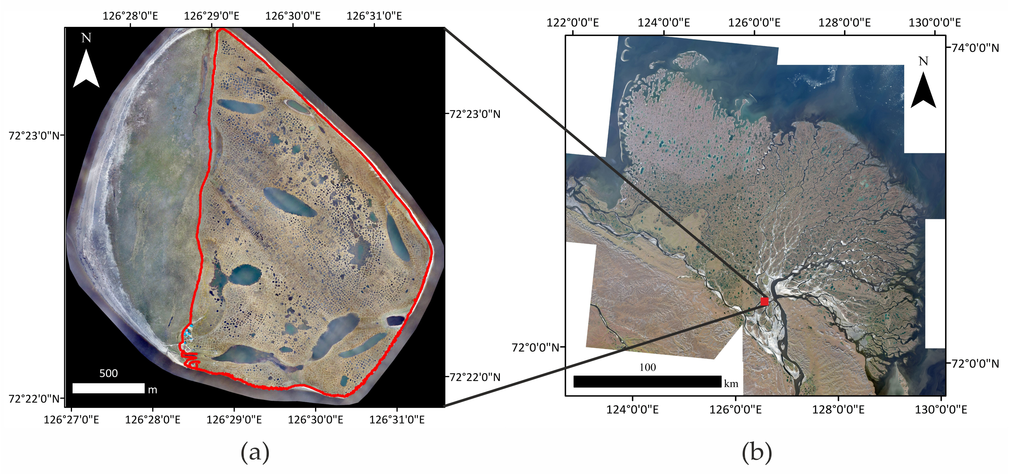
2. Study Area

The Lena River Delta (Figure 1b) is the largest Arctic river delta in the world. The total area of the entire Lena Delta is about 29,278 km² [25], with an average annual discharge of about 513 km³ [26]. The Lena Delta is traditionally subdivided into three terraces [27,28]. They differ by the sediments that constitute them, as well as by the age and sedimentation history in general. The first terrace is the youngest one that represents an active river delta and is a remnant of the Holocene stage of the delta formation [28,29]. This terrace reaches a height of 12 m a.s.l. and consists of organic-rich sands or silty-sandy peats [28,29]. The major part of the first terrace is located in the eastern part of the delta.

The second terrace is located in the western part of the delta. This terrace has a height of 20–30 m a.s.l. and is built of fluvial massive fine-grained deposits without silt, clay, or organic matter [28,30]. The deposition of these sediments mainly occurred in the marine isotope stage (MIS) 3 Interstadial and continued in the MIS 2 glacial period [30]. The third terrace is the oldest geomorphological level of the delta. This is an erosional remnant of a late Pleistocene broad foreland plain that was cut by Lena river branches [28,30,31,32]. This terrace is approximately 45–50 m a.s.l. and consists of Late Pleistocene–Holocene deposits [28,29,32]. In general, three members compose the late Pleistocene to Holocene sequence of the third terrace (from the bottom to the top in stratigraphic order, according to Wetterich et al. [32]): first – Early Weichselian fluvial sands, second – Middle-Late Weichselian Ice complex deposits (Edoma), and third – Holocene peaty and sandy silts with peat lenses and plant detritus. These members were revealed and studied in coastal exposures of the south-eastern part of Kurungnakh Island by Wetterich et al. [32]. The origin and age relationship between these terraces are debatable and were not the object of our study. Geomorphological distinguishing features of the first terrace is the presence of a Holocene ice wedge network; elongated lakes, which are remnants of old channels; and the absence of oriented thermokarst lakes (as differentiated from the second terrace) and large isometric alases hundreds of meters wide (as distinct from the third terrace).

Samoylov Island (72.374528° N, 126.490289° E) is located in the south-eastern part of the Lena River Delta, within the continuous permafrost zone. Permafrost thicknesses of this territory are 400–600 m [33]. Boike et al. [34] present detailed data about climate, permafrost, and active layer conditions. The coldest month in the study area is February, with mean monthly air temperature of −32.7 °C (−25.6 °F), whilst the warmest month is July, with a mean of 9.5 °C (48.2 °F). Mean annual air temperature is −12.3 °C (10.4 °F) [34]. The active layer thawing period lasts from the end of May until the end of August or beginning of September.

Samoylov Island (Figure 1a) consists of two major geological and geomorphological components. These include the first terrace (eastern part of the island) and a floodplain (western part of the island). These surfaces are easily recognizable, even on small-scale RS data, and vary in landform morphological properties. The first terrace consists of ice-rich alluvial deposits, which range from organic-rich sands at the bottom, to silty-sandy peats towards the surface [28]. Average ice content in the upper meter of the first terrace is >65% [35] and the thickness of the active layer of the first terrace reaches about 30–50 cm. A distinctive feature of the first terrace is the ice wedges, which have a polygonal shape and comprise a sizeable volume of ground ice of the first terrace. Ice wedges are absent on the western floodplain part of the island. Ice content in the upper meter of the floodplain is about 35% [35]. Typical sandy facies of river deposits comprise the floodplain. As it is the active delta floodplain, the active layer thickness of this surface can reach more than 1 m.

The Laptev Sea region is experiencing active warming, determined using borehole temperature measurements [34]. According to Boike et al. [34], the permafrost temperature on Samoylov Island has increased by as much as 1.3 °C at the zero amplitude depth of 20.75 m since the start of observations in 2006. As a consequence, the presence of various degrading polygonal nets, exhaustive data about environmental conditions and geology of the deposits, and ongoing landscape degradation due to global warming make the study area an ideal site for investigations of landscape change as a result of active permafrost degradation.

3. Materials and Methods

3.1. UAV Imaging and Photogrammetry

UAV-based imaging was conducted at the end of July 2016 in a summer field expedition. We used a Supercam S 250 UAV manufactured by "Unmanned Systems" LLC, 2, Ordzhonikidze St., Izhevsk, Russian Federation, which was equipped with a geodetic-class GPS receiver and a Sony Alpha 6000 24.7 MP APS-C digital camera. Aerial images of Samoylov Island were captured at an altitude of about 150 m above ground level, with a total UAV flight time of 1 hour and 32 minutes. A total of 3743 images were captured, which cover 4.4 km² of the island. We designed the flight grid based on the desired resolution of the orthophoto map, ground conditions, and total area of the island. Before the UAV flight, we set up the base station network for precise GPS measurements and as a reference point network. A set of objects that were easily visible to the aircraft’s digital camera from the intended flight altitude were placed on the ground and then mapped with a geodetic-class GPS receiver.

We used specialized software for photogrammetry: Agisoft PhotoScan (Professional Edition, Version 1.2.5) from Geoscan Ltd. and Photomod package (version 5.0) from JSC Racurs. As the basis for rectification, we used picture center coordinates and coordinates of ground reference points. Due to the lack of natural or manmade objects suitable for serving as reference points, we made an even grid of such marks ourselves and then performed high-precision GPS mapping on them. As a result of the photogrammetry, we received 29 georeferenced orthophoto map tiles with a 0.05 m/px resolution and a digital terrain model (DTM) presented using a height matrix. The horizontal resolution of the DTM was 0.5 m/px and the vertical accuracy was 0.2 m. Each matrix cell contained planar coordinates and height values. An important feature of the data obtained in the Lena Delta region was the large volume of water surfaces. As a result, we had to perform the tedious task of manually contouring these water surfaces and accounting for them in the DTM. This was due to limitations in the current state of photogrammetry software and its inability to correctly process regions in stereo pairs that contain uniform pixel clusters. As a result, in the automatic switching mode, the software produces significant height noise in such regions. This problem also cannot be solved with automatic filtering. Therefore, we had to manually outline (vectorize) all water bodies, arbitrarily determine water level height using a spatial model, and set this water level for each water body. It should be noted that the elevation of water bodies was not an objective of our study, therefore any small inaccuracies in the assignment of these elevations did not influence our investigation.

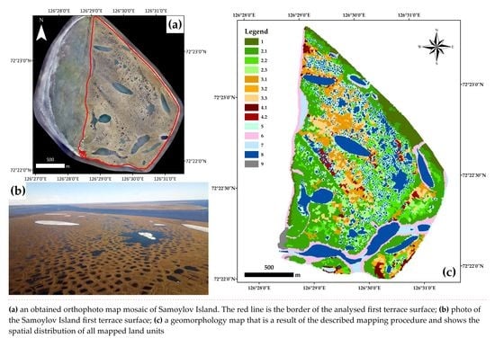
3.2. GIS Analysis and Geomorphological Mapping

Obtained orthophoto maps (Figure 1a) and DTM (Figure 2a) were analyzed in the GIS software package ArcGIS 10.2.2 from ESRI CIS Limited. We used the GIS analysis for creating several maps of land morphometry parameters, such as shaded relief (Figure 2b), slope (Figure 2c), and aspect (Figure 2d and Figure 3b) maps. Also, we created various mean DTM maps, which were derived from DTM averaging with a moving window of 20, 30, 40, and 50 m. Moreover, we created a map of local differentiation of the relief by subtracting the actual DTM from the mean DTM. Figure 4b,c, as well as their description, show the example of using this map.

In accordance with classical theory, there are two types of ice wedge polygons: low-centered and high-centered [2,12,36,37,38]. The former corresponds to the growth of ramparts adjacent to the thermal contraction cracks, and the latter is a result of thermokarst degradation along ice wedges [2]. However, the relationship between steps of degradation and polygon topography was not well understood until recently. Several models for ice wedge polygon degradation have been developed in recent years, which have enhanced our understanding of this relationship. For example, there is a hydrological model simulation of degradation that describes a change of tundra water balance due to changes in snow distribution as a result of the formation of troughs on the land surface [5]. Kanevskiy et al. [8] developed new conceptual models of ice wedge dynamics and determined the main stages of polygon degradation and stabilization based on comprehensive field work and various analyses. There are also a number of linked studies and models [8,9,10,11,39,40,41]. Nitzbon et al. [6] further developed the model on the basis of field measurements from Samoylov Island. This is very important for our study because this new model compliments previous models and studies, and is also based on Samoylov Island field measurements. In addition, polygon degradation simulation by Nitzbon et al. [6] corresponds well with models by Kanevskiy et al. [8] and Jorgenson et al. [9]. All these models describe polygon degradation as cycles of evolution, which can repeat several times after periods of stabilization, unlike the hydrological model of Liljedahl et al. [5], which describes polygon degradation as a single unidirectional evolutionary process.

We aimed to identify types of polygons, which were easily recognizable and can be used in further analysis in most of the aforementioned models. Our polygon types distinctly corresponded to different stages of degradation in the various models and we used the simplest topography classification of polygons [12]. We also took into account the presence or absence of water in the center of polygons and troughs. Therefore, we have recognized different types of polygons, water bodies, and other land units using manual mapping based on specific topographic and visual properties of each recognized land unit. We made two perpendicular topographic profiles, and analyzed morphometric and visual characteristics of all Samoylov Island polygons to determine their type. We used only manual methods of mapping, which as well as a high spatial resolution of RS data, allowed for a high degree of accuracy in the identification of all land units. We also mapped other geomorphological units, such as hillslopes, erosional valleys, and water bodies. The identified land units and their characteristics are described further in the results.

4. Results

We identified and mapped the following land units based on the aforementioned mapping procedure.

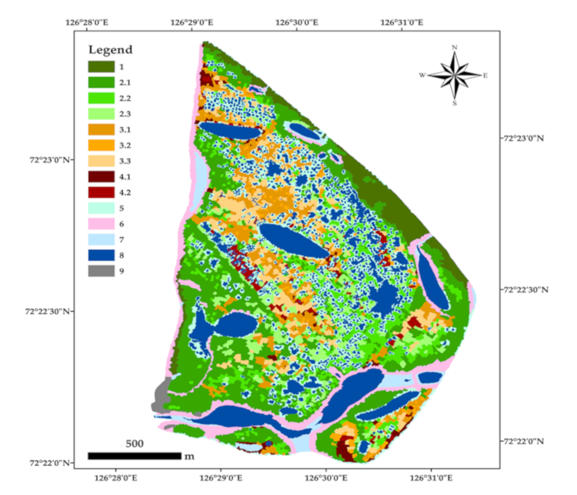
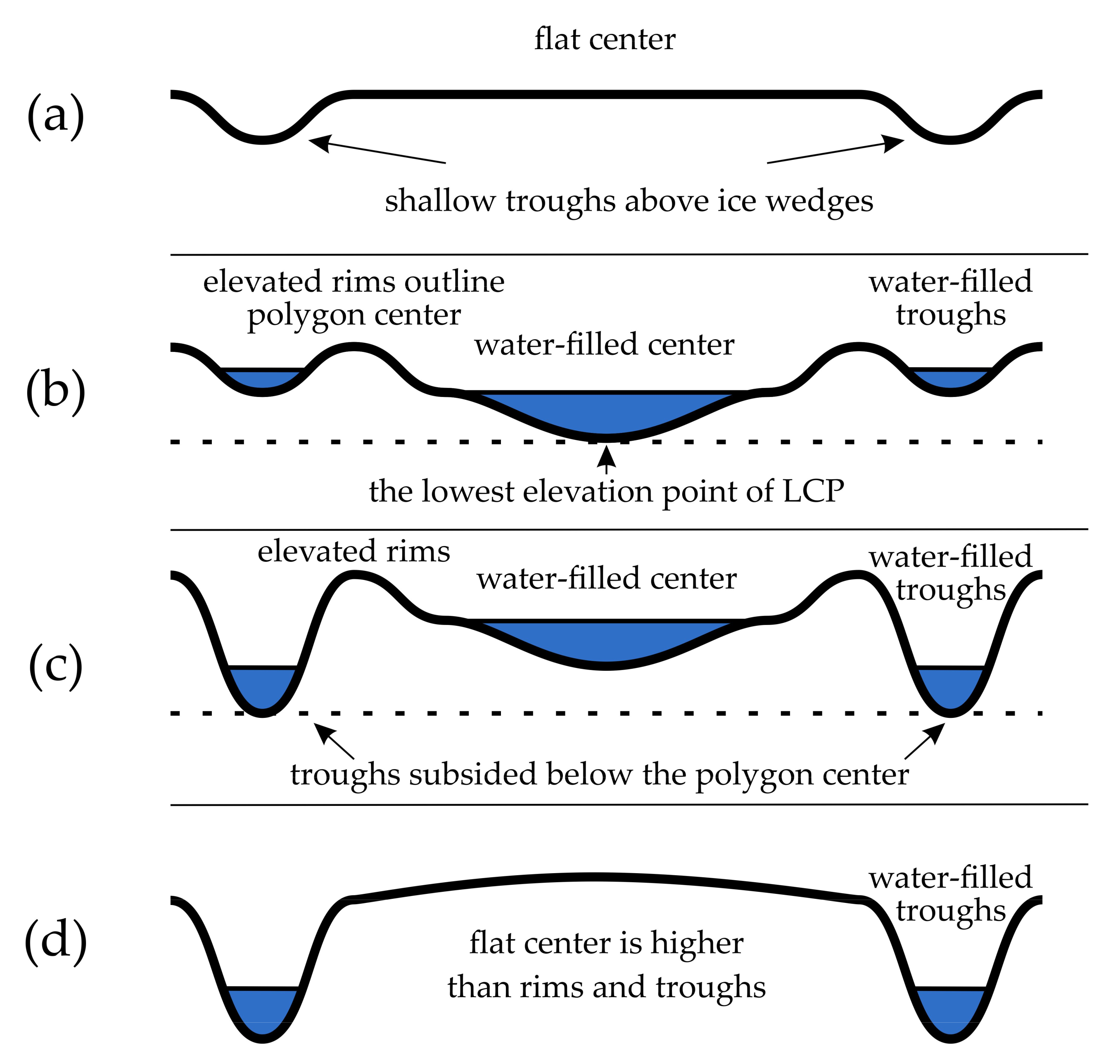
• Incipient polygons (IP): These represent drained polygons with flat centers, an absence of rims, and rather shallow troughs (10–20 cm) above ice wedges (Figure 3 and Figure A1a). Incipient polygons are the start point of polygon development and their further degradation. They usually arise on newly exposed ground, for example, on the bottom of drained lakes [12].
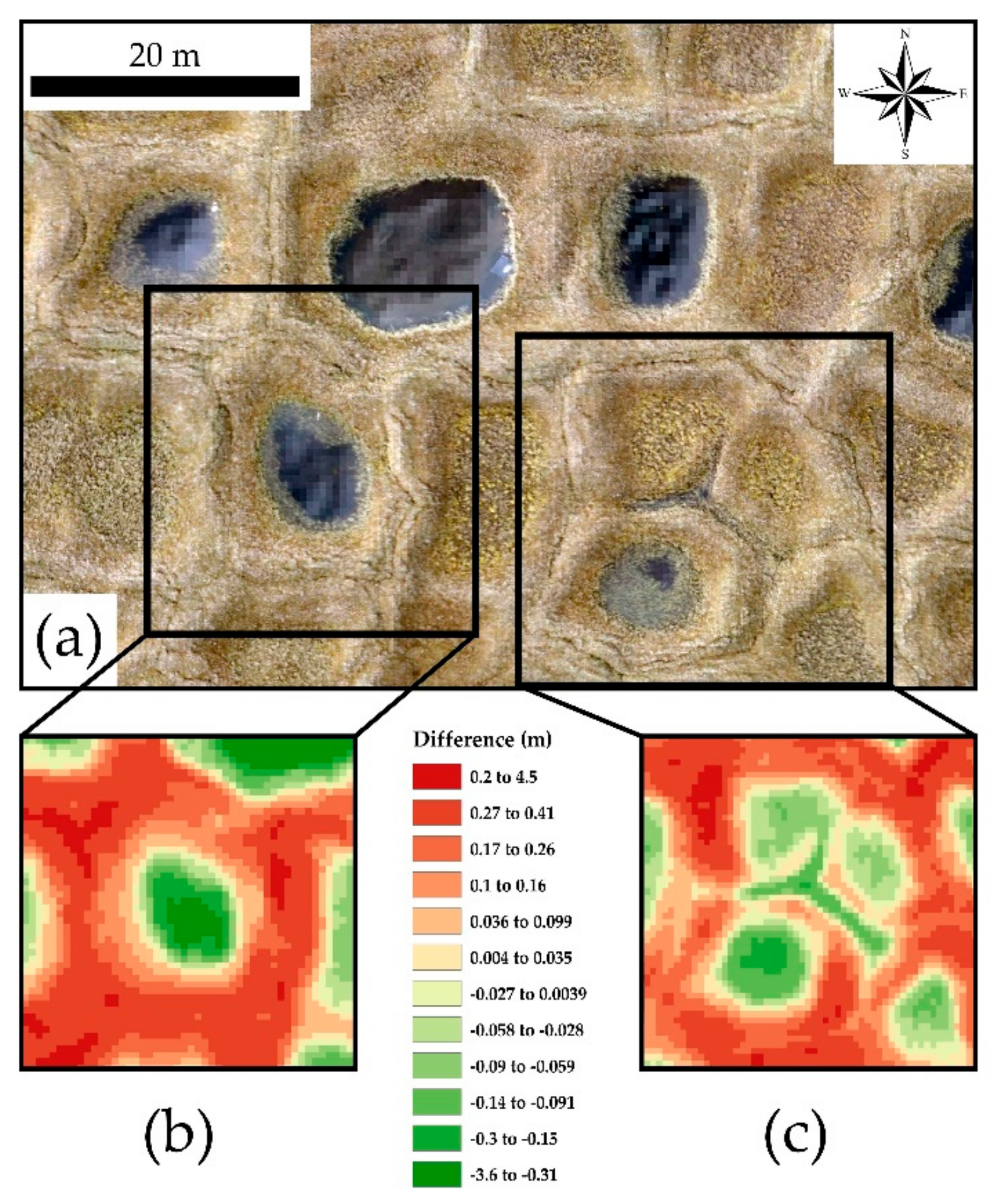
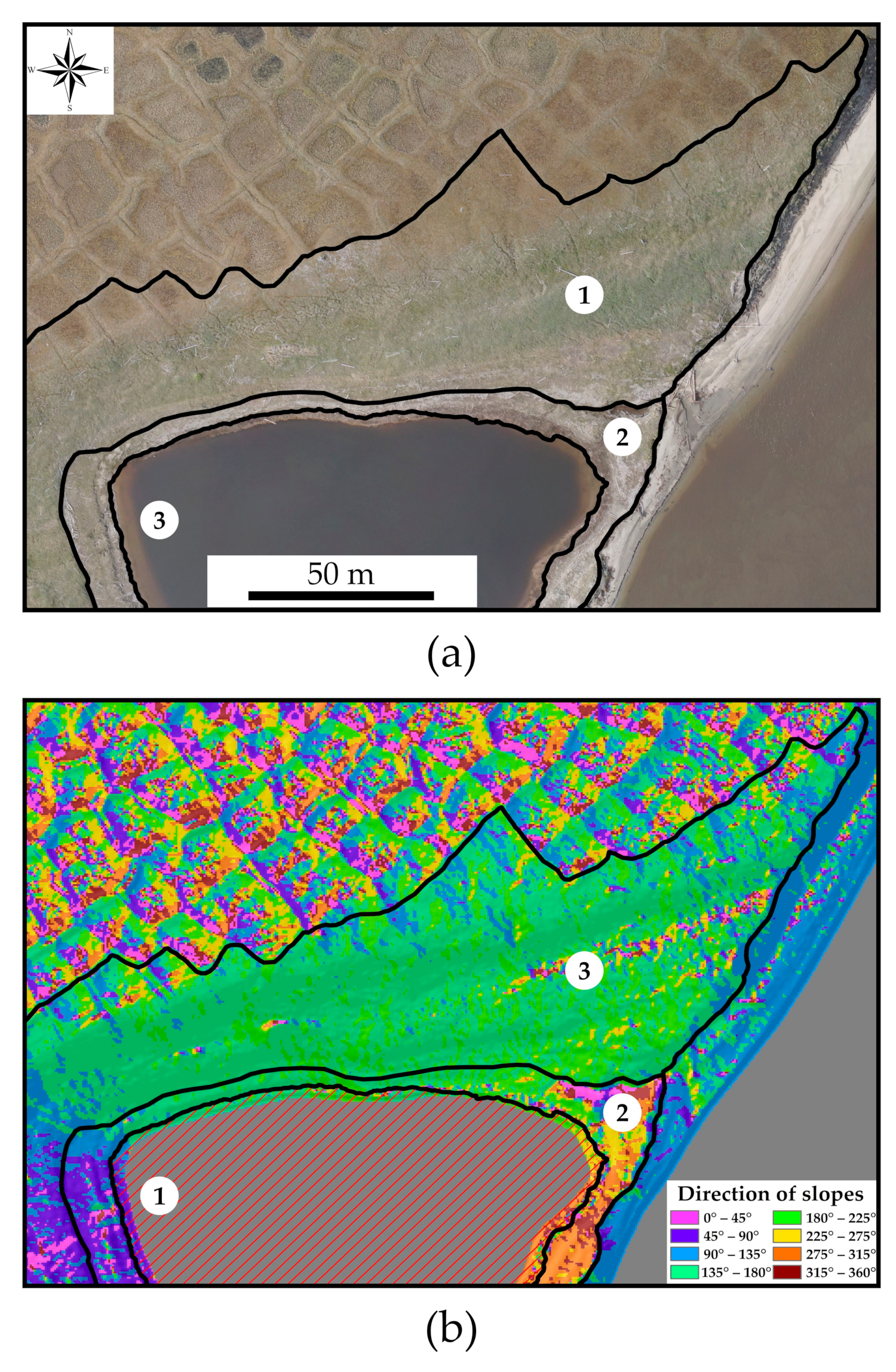
• Low-centered polygons (LCP): In accordance with French [2], Mackay [12], Liljedahl et al. [5], and Nitzbon et al. [6], we designated this type of polygon as having the lowest elevation point in the center (Figure 4 and Figure A1b). Elevated rims, or ramparts, outline polygon centers. Nevertheless, the elevation of troughs was greater than polygon centers. Besides low-centered polygons (2.1), we have revealed low-centered polygons with water-filled centers (2.2) and with water-filled troughs (2.3), because the presence of water can change the hydrological regime of polygon nets and lead to the onset of thermokarst activity. This process is described in the aforementioned models of polygon degradation.
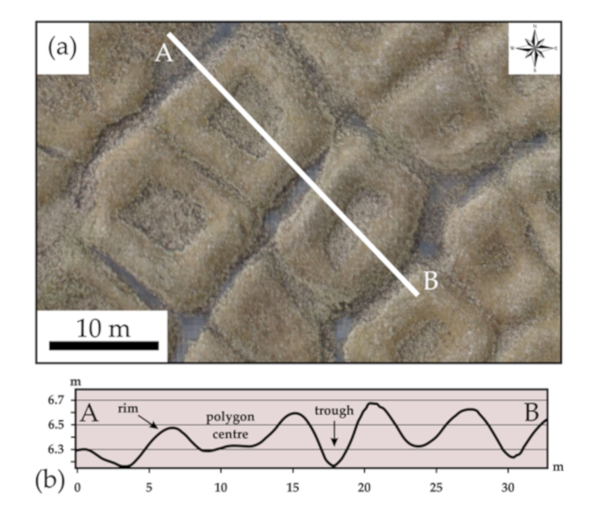
• Intermediate-centered polygons (ICP): We have recognized polygons with troughs, which subsided below the polygon centers, but with elevated rims (Figure 5 and Figure A1c). Polygons with these topographic characteristics were named “intermediate-centered” in Nitzbon et al. [6], although Root [42], Mackay [12], and French [2] named this type as walled or fortress polygons. In any case, the topography of ICP usually represents a further step of degradation after LCP. As for LCP, we subdivided ICP into three land units: intermediate-centered polygons (3.1), intermediate-centered polygons with water-filled centers (3.2), and intermediate-centered polygons with water-filled troughs (3.3). It should be noted that in some cases, polygons of land units 2.3 and 3.3 also have water-filled centers. However, we decided that the presence of water in troughs is more important, as connected troughs can lead to the destruction of polygon rims and the lateral expansion of ponds, which have appeared already or will do so in the future.
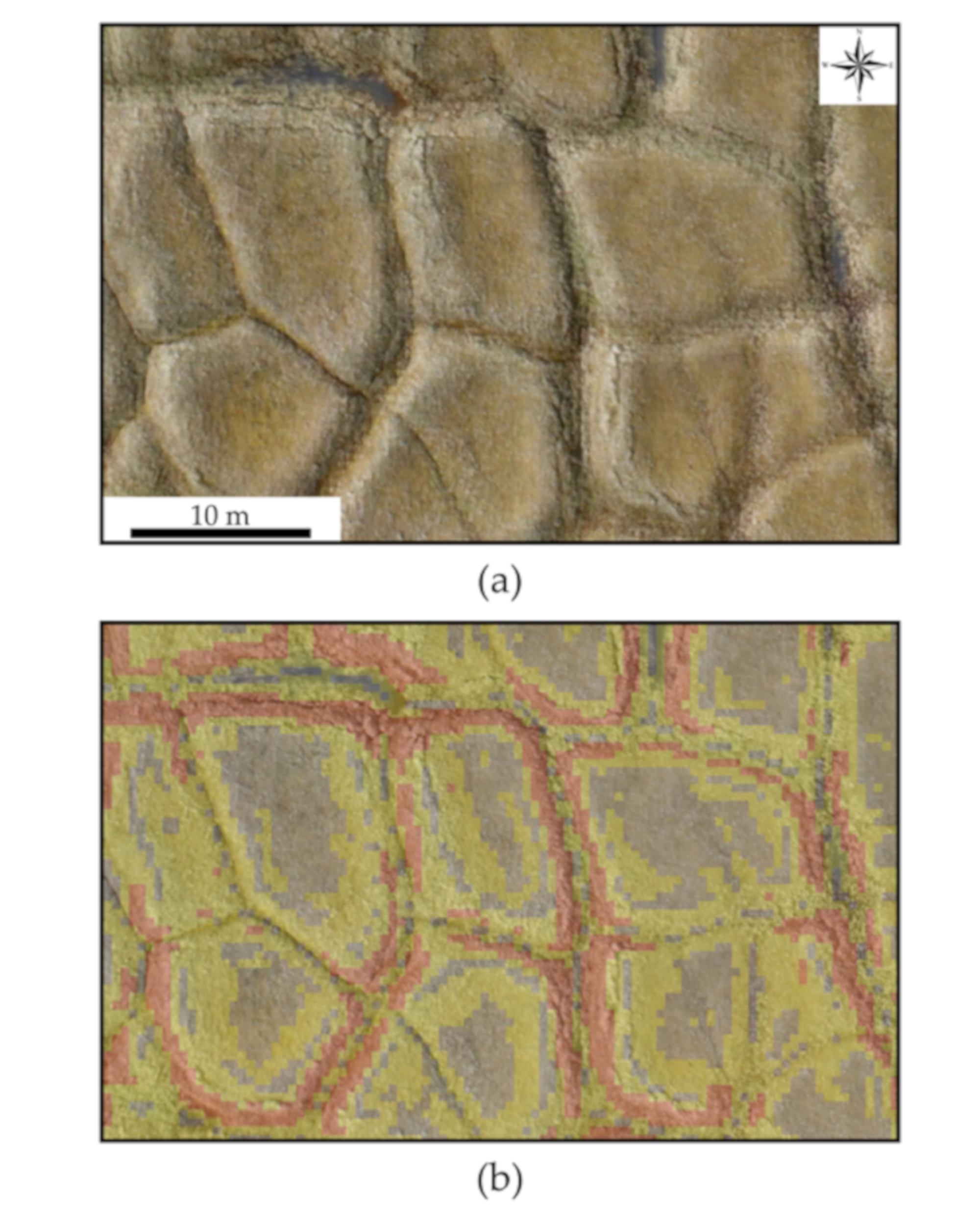
• High-centered polygons (HCP): We have named polygons with flat centers, which are higher than rims and troughs, as HCP (Figure 6 and Figure A1d). In some cases, rims of HCP are slightly elevated (5–10 cm), but are not higher than the polygon center. Nevertheless, the distinctive feature of HCP is the absence of any depression in the polygon center. This topographic characteristic does not allow for the development of ponds in the polygon centers. Depths of HCP troughs vary from 0.2–0.3 m to 1–1.2 m in different parts of the island. We also recognized high-centered polygons (4.1) and high-centered polygons with water-filled troughs (4.2).
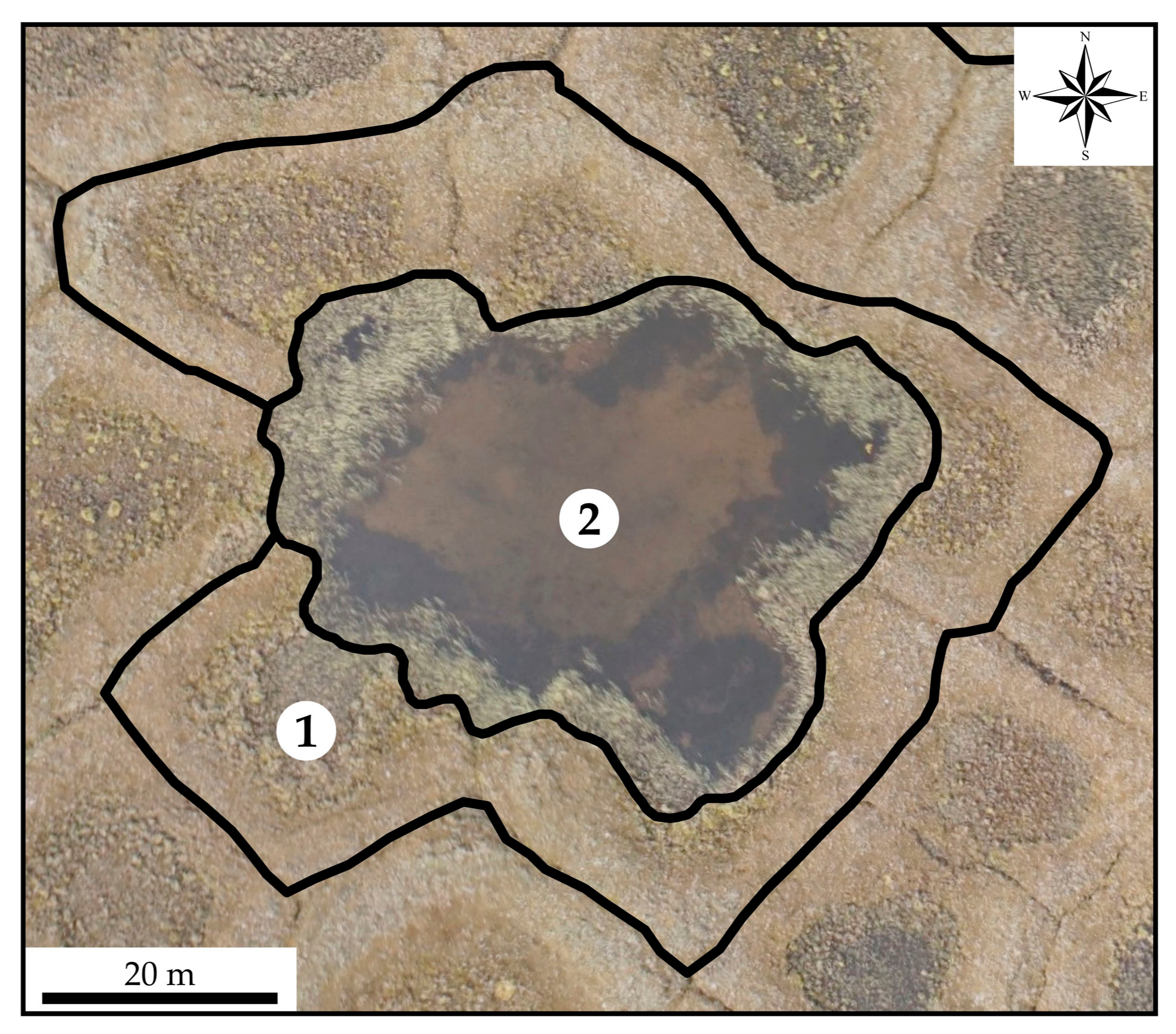
• Collapsed polygons (CP) (Figure 7): We observed destroyed polygons in the wettest parts of the island. Ponds of these polygons have merged and identification of the original type of polygon was problematic. In addition, we assigned polygon remnants around and in water bodies as CP.
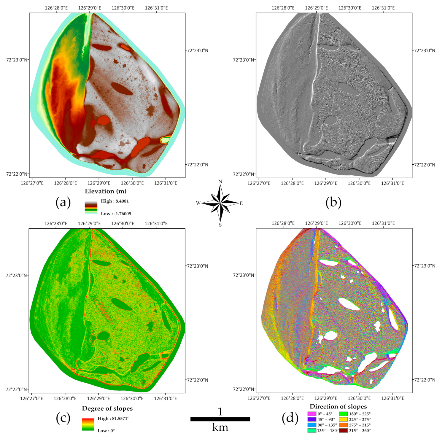
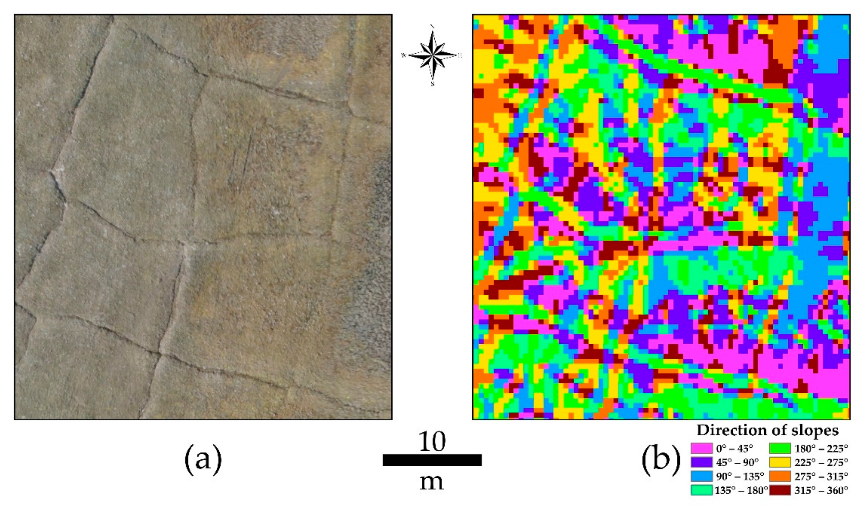
• Slopes: All slopes were easily recognizable in all morphometry schemes, especially in aspect schemes (Figure 8). When the slope angle increases to >2°, solifluction processes occur, changing the microtopography and destroying polygons. Moreover, slopes have a distinct vegetation cover, which simplifies their recognition in orthophotos. Some IP have been observed on slopes, but we concluded that slope processes play the main role in the topography change of this territory. Furthermore, polygons located on slopes were either degraded already, or will be degraded by solifluction over time. Therefore, these polygons did not follow the models for polygon evolution.
• Valleys (Figure 8): Floods erode valleys during the spring season. Valleys subside due to thermal and fluvial erosion and were overlapped by a thin layer of sandy or silty sediments from water currents. Some signs of polygon presence were observed on the flat bottom parts of valleys. However, floods cover these surfaces annually and their influence precluded the stabilization or growth of ice wedges. Therefore, we have not found any IP on valley bottoms.
• Lakes and other water bodies (Figure 7 and Figure 8): Clear distinctions and differences between merged polygon ponds and small thermokarst lakes, which developed in troughs via polygon degradation, were problematic. The largest lakes often connected with surrounding shallow ponds, and borders between these water bodies were also difficult to determine. We have therefore unified large lakes, and merged polygon ponds and water-filled troughs, if they eroded more than half of adjacent polygons, as one land unit. We have identified all water bodies in orthophotos.
• The Samoylov Island research station: A number of station buildings are located in the south-western part of the study area. The presence of infrastructure complicates our geomorphological analysis of this terrain, therefore we excluded this terrain from further assessment.

Figure 9 represents the spatial distribution of all aforementioned mapped land units. Following identification and mapping, we calculated the distribution area of each land unit (

Table 1. The distribution area of each land units (without the Samoylov Island research station) and their percentages.

	Land Units	m2	%
1	Incipient polygons (IP)	136,242	4.82%
2.1	Low-centered polygons (LCP)	658,787	23.30%
2.2	LCP with water-filled centers	218,520	7.73%
2.3	LCP with water-filled troughs	168,144	5.95%
3.1	Intermediate-centered polygons (ICP)	213,881	7.55%
3.2	ICP with water-filled centers	46,979.1	1.66%
3.3	ICP with water-filled troughs	174,479	6.17%
4.1	High-centered polygons (HCP)	39,804.1	1.41%
4.2	HCP with water-filled troughs	44,199.2	1.56%
5	Collapsed polygons (CP)	325,495	11.51%
6	Slopes	193,354	6.84%
7	Valleys	66,706.4	2.36%
8	Lakes and other water bodies	541,209	19.14%

) using the GIS software package ArcGIS 10.2.2 by ESRI. The accuracy of the results in Figure 9 and Table 1 is within 5 cm since only the resolution of orthophoto map tiles limited the accuracy of manual mapping. The total area of the mapped study site was 2.844951 km². We excluded the Samoylov Island research station (17,152 m²) from this number, and estimated the land unit areas and their percentages.

5. Discussion

IP occupied 136,242 m² (4.82%) of the first terrace surface and were only found across the north-eastern edge of Samoylov Island. Their distribution was connected with the continual deposition of sands during the highest floods, which overlapped the first terrace deposits and ice wedges. Furthermore, wind activity transported sand around 20–30 m in an inland direction. This process occurred when river ice eroded vegetation cover and exposed sandy sediments. After some time, vegetation covered this territory again and ice wedges appeared as an incipient polygon net.

About a quarter of the study area was occupied by LCP (658,787 m²; 23.30%). These polygons represented the first stage of polygon degradation according to modern models [5,6,8,9,11] and traditional views [2,12]. However, further degradation from this stage depended on the hydrological regime, especially the presence of water in the centers and troughs of polygons. Water-filled troughs led to melting of ice wedges and the appearance of ICP, while ponds in polygon centers could lead to their melting and subsidence. Future degradation also depended on many other conditions, such as climate; however, the presence of water was an important prerequisite for further degradation. Therefore, accurate estimation of LCP with water-filled centers (218,520 m²; 7.73%) and LCP with water-filled troughs (168,144 m²; 5.95%) is very important for further predictions of degradation based on each model.

The area covered with ICP topography was 213,881 m² (7.55%). These polygons were mainly located in the depressed central part of the island where they surround water bodies and collapsed polygons. The presence of water and extreme meteorological conditions [10] control their distribution. These polygons could become stable in the absence of water, while the presence of water in ICP with water-filled centers (46,979.1 m²; 1.66%) and LCP with water-filled troughs (174,479 m²; 6.17%) could facilitate continued degradation. Nonetheless, this mapped area of the island represented another stage of polygon degradation and contributed to the percentage of changed area via thermokarst activity.

The other two types of degraded polygons (HCP: 39,804.1 m², and HCP with water-filled troughs: 44,199.2 m²) occupied <3% of the study area. HCP are primarily situated in well-drained local depressions, where ice wedge melting occurred rapidly without polygon center subsidence. In contrast, HCP with water-filled troughs were observed in the poorly-drained central part of the island. Nitzbon et al. [6] concluded that well-drained polygons in the northern part of the island could be described, according to Liljedahl et al. [5], as a final stage of polygon degradation (HCP). Nitzbon et al. [6] revealed that these polygons relate to the final equilibrium state, which corresponds well with other models [8,9]. Therefore, polygons with the same topography may be attributed to different degradation stages in different models. However, our mapped geomorphological units conformed to specific microtopography characteristics and hydrological conditions; therefore, they may be used during further studies independently of the used model of polygon degradation and are applicable to various modern models.

One of the most widespread land units were collapsed polygons (325,495 m²; 11.51%). These had almost completely degraded and were located beside water bodies of various scales. Due to the continued influence of water, we predict that these polygons will be degraded completely under the influence of continued thermokarst activity, coastal processes, and solifluction. Similarly, slopes (193,354 m²; 6.84%) and valleys (66,706.4 m²; 2.36%) also represented degraded thermokarst landscapes under the influence of different thermokarst processes; however, the polygonal tundra of these features was completely eroded. These land units could therefore be classified as the final stages of polygon degradation. The accurate mapping of slopes and identification of their orientation relative to the sun, wind, or hydrological regime, allow us to make further studies on thermokarst activity in the study area. Furthermore, this method and the results of slope mapping show the potential of using UAV data for analyzing slope dynamics.

Water bodies (541,209 m²; 19.14%) occupied one fifth of the first terrace surface of Samoylov Island. According to previous studies, water surfaces occupy 25% of the area [43], and 35% of the polygonal tundra on Samoylov Island is occupied by polygonal ponds and troughs [44]. Muster et al. [43] also estimated proportions of the island that are composed of dry tundra (58%) and wet tundra (17%) based on RS data and field measurements. Unfortunately, we cannot directly compare our data with these because we did not estimate areas of individual polygon ponds or obtain field measurements. However, our high-resolution estimation shows the proportion of degraded area, which on the one hand was infilled by water, and on the other hand, will tend to increase in the near future.

Therefore, in accordance with our results and estimation, non-degraded polygonal tundra (IC and all types of LCP) comprised an area of 1,181,693 m², representing 41.79% of the first terrace surface. However, it should be noticed that this number includes polygons showing early signs of degradation (LCP with water-filled centers and troughs, 2.2, and 2.3), which comprise 386,664 m² (13.67%) of the studied area. The area that is comprised of already degraded polygons (all types of ICP and HCP) covered 519,342.4 m², representing 18.37% of the first terrace surface. Since one type of polygon microtopography may be referred to as various stages of degradation in different models, we did not subdivide the study area into areas with different stages of polygon degradation in accordance with the aforementioned models. However, our estimation shows the modern status of polygonal tundra degradation on Samoylov Island and our results are applicable for future studies of polygon evolution independent of the model used. In addition, we estimated that 1,126,764.4 m² (39.84%) of the studied area comprised absolutely or almost completely degraded polygonal tundra (CP, slopes, valleys, lakes, and other water bodies). Not all of this territory was composed of ice wedge polygons; however, it is clear that a primordial tundra landscape was degraded here, and its future evolution depends on climate, hydrological factors, and many other conditions. As a result, our results and discussion prove that future monitoring of landscape dynamics by means of GIS analysis of UAV data, in this study area or elsewhere with a periglacial environment, is possible and informative.

6. Conclusions

We identified morphometric characteristics of land units and manually mapped them using UAV data analyzed in GIS. Further estimation of their distribution across the study area revealed the modern status of landscape evolution and polygonal tundra degradation. Modern models for polygon degradation were characterized by significant differences; therefore, we have not tried to assign each of our identified polygon types to an evolutionary succession in one of the existing models. Our study revealed that 41.79% of the first terrace surface was composed of non-degraded polygonal tundra; 18.37% was composed of polygons that had signs of thermokarst activity and corresponded to various stages of degradation in the models; and 39.84% was composed of collapsed polygons, slopes, valleys, and water bodies, excluding ponds of individual polygons. This latter group corresponded to the final steps of permafrost and landscape degradation. Our revealed land units are multi-purpose and could be used in a number of future studies, including the prediction of future landscape dynamics based on different models.

Therefore, from our study we can make the following conclusions. First, this investigation shows the modern status of polygonal tundra degradation of the first terrace surface on Samoylov Island. Our assessment could be extrapolated to adjacent islands and reflect the landscape condition of the first terrace surface across the southern part of the Lena Delta. Second, the method of UAV data analysis in GIS could be used in scientific studies for monitoring Arctic landscape changes under the influence of global warming, as well as during geoengineering studies, related to hazard assessment of permafrost degradation for infrastructure.

References

- Walker, D.A.; Raynolds, M.K.; Daniëls, F.J.; Einarsson, E.; Elvebakk, A.; Gould, W.A.; Katenin, A.E.; Kholod, S.S.; Markon, C.J.; Melnikov, E.S.; et al. The circumpolar Arctic vegetation map. J. Veg. 2005, 16, 267–282. [Google Scholar] [CrossRef]
- French, H.M. The Periglacial Environment, 3rd ed.; John Wiley & Sons: West Sussex, UK, 2007; p. 458. [Google Scholar]
- Leffingwell, E.K. Ground-ice wedges: the dominant form of ground-ice on the north coast of Alaska. J. Geol. 1915, 23, 635–654. [Google Scholar] [CrossRef]
- Lachenbruch, A.H. Mechanics of thermal contraction cracks and ice-wedge polygons in permafrost. In GSA Special Papers; Geological Society of America: Boulder, CO, USA, 1962. [Google Scholar] [CrossRef]
- Liljedahl, A.K.; Boike, J.; Daanen, R.P.; Fedorov, A.N.; Frost, G.V.; Grosse, G.; Hinzman, L.D.; Iijma, Y.; Jorgenson, J.C.; Matveyeva, N.; et al. Pan-Arctic Ice-Wedge Degradation in Warming Permafrost and Its Influence on Tundra Hydrology. Nat. Geosci. 2016, 9, 312–318. [Google Scholar] [CrossRef]
- Nitzbon, J.; Langer, M.; Westermann, S.; Martin, L.; Aas, K.S.; Boike, J. Pathways of ice-wedge degradation in polygonal tundra under different hydrological conditions. Cryosphere 2019, 13, 1089–1123. [Google Scholar] [CrossRef]
- Jorgenson, M.T.; Shur, Y.L.; Pullman, E.R. Abrupt increase in permafrost degradation in Arctic Alaska. Geophys. Res. Lett. 2006, 33, 2–5. [Google Scholar] [CrossRef]
- Kanevskiy, M.; Shur, Y.; Jorgenson, T.; Brown, D.R.N.; Moskalenko, N.; Brown, J.; Walker, D.A.; Raynolds, M.K.; Buchhorn, M. Degradation and stabilization of ice wedges: implications for assessing risk of thermokarst in Northern Alaska. Geomorphology 2017, 297, 20–42. [Google Scholar] [CrossRef]
- Jorgenson, M.T.; Kanevskiy, M.; Shur, Y.; Moskalenko, N.; Brown, D.R.N.; Wickland, K.; Striegl, R.; Koch, J. Role of ground ice dynamics and ecological feedbacks in recent ice wedge degradation and stabilization. J. Geophys. Res. Earth Surf. 2015, 120, 2280–2297. [Google Scholar] [CrossRef]
- Abolt, C.J.; Young, M.H.; Atchley, A.L.; Harp, D.R. Microtopographic control on the ground thermal regime in ice wedge polygons. Cryosphere 2018, 12, 1957–1968. [Google Scholar] [CrossRef]
- Aas, K.S.; Martin, L.; Nitzbon, J.; Langer, M.; Boike, J.; Lee, H.; Berntsen, T.K.; Westermann, S. Thaw processes in ice-rich permafrost landscapes represented with laterally coupled tiles in a land surface model. Cryosphere 2019, 13, 591–609. [Google Scholar] [CrossRef]
- Mackay, J.R. Thermally induced movements in ice-wedge polygons, western arctic coast: A long-term study. Geogr. Phys. Quatern. 2000, 54, 41–68. [Google Scholar] [CrossRef]
- Zimov, S.A. Climate change: permafrost and the global carbon budget. Science 2006, 312, 1612–1613. [Google Scholar] [CrossRef] [PubMed]
- Tamocai, C.; Canadell, J.G.; Schuur, E.A.G.; Kuhry, P.; Mazhitova, G.; Zimov, S. Soil organic carbon pools in the Northern circumpolar permafrost region. Global Biogeochem. Cycles 2009, 23, 1–11. [Google Scholar] [CrossRef]
- Iwasaki, S.; Desyatkin, A.R.; Filippov, N.V.; Desyatkin, R.V.; Hatano, R. Carbon stock estimation and changes associated with thermokarst activity, forest disturbance, and land use changes in Eastern Siberia. Geoderma Reg. 2018, 14, e00171. [Google Scholar] [CrossRef]
- Anisimov, O.; Belolutskaya Grigoriev, A.I.; Kokorev, V.; Oberman; Reneva; Strelchenko, S.A.; Streletskiy, D.; Shiklomanov, N. Major Natural and Social-Economic Consequences of Climate Change in the Permafrost Region: Predictions Based on Observations and Modeling; Greenpeace: Moscow, Russia, 2010; p. 44. (In Russian) [Google Scholar]
- Streletskiy, D.; Anisimov, O.; Vasiliev, A. Permafrost Degradation. In Snow and Ice-Related Hazards, Risks, and Disasters; Shroder, J.F., Haeberli, W., et al., Eds.; Academic Press: Boston, MA, USA, 2015. [Google Scholar]
- Mora, C.; Lousada, M.; Pina, P.; Bandeira, L.; Vieira, G. Evaluation of the use of very high resolution aerial imagery for accurate ice-wedge polygon mapping (Adventdalen, Svalbard). Sci. Total Environ. 2017, 615, 1574–1583. [Google Scholar] [CrossRef]
- Fraser, R.H.; Olthof, I.; Lantz, T.C.; Schmitt, C. UAV Photogrammetry for Mapping Vegetation in the Low-Arctic. Arct. Sci. 2016, 2, 79–102. [Google Scholar] [CrossRef]
- Armstrong, L.; Lacelle, D.; Fraser, R.H.; Kokelj, S.; Knudby, A. Thaw Slump Activity Measured Using Stationary Cameras in Time-Lapse and Structure-from-Motion Photogrammetry. Arct. Sci. 2018, 4, 827–845. [Google Scholar] [CrossRef]
- Van der Sluijs, J.; Kokelj, V.S.; Fraser, H.R.; Tunnicliffe, J.; Lacelle, D. Permafrost Terrain Dynamics and Infrastructure Impacts Revealed by UAV Photogrammetry and Thermal Imaging. Remote Sens. 2018, 10, 1734. [Google Scholar] [CrossRef]
- Huang, L.; Liu, L.; Jiang, L.; Zhang, T. Automatic Mapping of Thermokarst Landforms from Remote Sensing Images Using Deep Learning: A Case Study in the Northeastern Tibetan Plateau. Remote Sens. 2018, 10, 2067. [Google Scholar] [CrossRef]
- Riihimäki, H.; Luoto, M.; Heiskanen, J. Estimating Fractional Cover of Tundra Vegetation at Multiple Scales Using Unmanned Aerial Systems and Optical Satellite Data. Remote Sens. Environ. 2019, 224, 119–132. [Google Scholar] [CrossRef]
- Saito, H.; Iijima, Y.; Basharin, N.I.; Fedorov, A.N.; Kunitsky, V.V. Thermokarst development detected from high-definition topographic data in Central Yakutia. Remote Sens. 2018, 10, 1579. [Google Scholar] [CrossRef]
- Kravtsova, V.I.; Mit’kinykh, N.S. Mouths of World Rivers in the Atlas of Space Images. Water Resour. 2011, 38, 1–17. [Google Scholar] [CrossRef]
- Degtyarev, V. Lena River Delta (Russia). In The Wetland Book: II: Distribution, Description, and Conservation; Finlayson, C.M., Milton, R., Prentice, C., Davidson, N.C., Eds.; Springer Netherlands: Dordrecht, The Netherlands, 2018; pp. 1451–1456. [Google Scholar]
- Grigoriev, M.N. Criomorphogenesis in the Lena Delta; Permafrost Institute Press: Yakutsk, Russia, 1993; p. 176. (In Russian) [Google Scholar]
- Schwamborn, G.; Rachold, V.; Grigoriev, M.N. Late Quaternary Sedimentation History of the Lena Delta. Quat. Int. 2002, 89, 119–134. [Google Scholar] [CrossRef]
- Bolshiyanov, D.; Makarov, A.; Savelieva, L. Lena River Delta Formation during the Holocene. Biogeosciences 2015, 12, 579–593. [Google Scholar] [CrossRef]
- Schirrmeister, L.; Grosse, G.; Schnelle, M.; Fuchs, M.; Krbetschek, M.; Ulrich, M.; Kunitsky, V.; Grigoriev, M.; Andreev, A.; Kienast, F.; et al. Late Quaternary Paleoenvironmental Records from the Western Lena Delta, Arctic Siberia. Palaeogeogr. Palaeoclimatol. Palaeoecol. 2011, 299, 175–196. [Google Scholar] [CrossRef]
- Schirrmeister, L.; Grosse, G.; Schwamborn, G.; Andreev, A.A.; Meyer, H.; Kunitsky, V.V.; Kuznetsova, T.V; Dorozhkina, M.V; Pavlova, E.Y.; Bobrov, A.A.; et al. Late Quaternary History of the Accumulation Plain North of the Chekanovsky Ridge (Lena Delta, Russia): A Multidisciplinary Approach. Polar Geogr. 2003, 27, 277–319. [Google Scholar] [CrossRef]
- Wetterich, S.; Kuzmina, S.; Andreev, A.A.; Kienast, F.; Meyer, H.; Schirrmeister, L.; Kuznetsova, T.; Sierralta, M. Palaeoenvironmental Dynamics Inferred from Late Quaternary Permafrost Deposits on Kurungnakh Island, Lena Delta, Northeast Siberia, Russia. Quat. Sci. Rev. 2008, 27, 1523–1540. [Google Scholar] [CrossRef]
- Grigoriev, N.F. The temperature of permafrost in the Lena delta basin–deposit conditions and properties of the permafrost in Yakutia. Yakutsk 1960, 2, 97–101. (In Russian) [Google Scholar]
- Boike, J.; Nitzbon, J.; Anders, K.; Grigoriev, M.; Bolshiyanov, D.; Langer, M.; Lange, S.; Bornemann, N.; Morgenstern, A.; Schreiber, P.; et al. A 16-Year Record (2002–2017) of Permafrost, Active-Layer, and Meteorological Conditions at the Samoylov Island Arctic Permafrost Research Site, Lena River Delta, Northern Siberia: An Opportunity to Validate Remote-Sensing Data and Land Surface, Snow, and Permafrost Models. Earth Syst. Sci. Data 2019, 11, 261–299. [Google Scholar] [CrossRef]
- Zubrzycki, S.; Kutzbach, L.; Grosse, G.; Desyatkin, A. Organic Carbon and Total Nitrogen Stocks in Soils of the Lena River Delta. Biogeosci. 2013, 10, 3507–3524. [Google Scholar] [CrossRef]
- Mackay, J.R. The Mackenzie Delta Area; Geographical Branch Memoir, no. 8; Queen’s printer: Ottawa, ON, Canada, 1963; p. 202. [Google Scholar]
- Hussey, K.M.; Michelson, R.W. Tundra relief features near Point Barrow, Alaska. Arctic 1966, 19, 162–184. [Google Scholar] [CrossRef]
- Romanovskiy, N.N. Formation of Polygonal-Wedge Structures; Nauka SSSR: Novosibirsk, Russia, 1977; p. 212. (In Russian) [Google Scholar]
- Kumar, J.; Collier, N.; Bisht, G.; Mills, R.T.; Thornton, P.E.; Iversen, C.M.; Romanovsky, V. Modeling the spatiotemporal variability in subsurface thermal regimes across a low-relief polygonal tundra landscape. Cryosphere 2016, 10, 2241–2274. [Google Scholar] [CrossRef]
- Grant, R.F.; Mekonnen, Z.A.; Riley, W.J.; Wainwright, H.M.; Graham, D.; Torn, M.S. Mathematical modelling of Arctic polygonal tundra with Ecosys: 1. Microtopography determines how active layer depths respond to changes in temperature and precipitation. J. Geophys. Res. Biogeosci. 2017, 122, 3161–3173. [Google Scholar] [CrossRef]
- Bisht, G.; Riley, W.J.; Wainwright, H.M.; Dafflon, B.; Fengming, Y.; Romanovsky, V.E. Impacts of microtopographic snow redistribution and lateral subsurface processes on hydrologic and thermal states in an arctic polygonal ground ecosystem: a case study using ELM-3D v1.0. Geosci. Model Dev. 2018, 11, 61–76. [Google Scholar] [CrossRef]
- Root, J.D. Ice-Wedge Polygons, Tuktoyaktuk Area, North –West Territories; Geology Survey of Canada: Ottawa, ON, Canada, 1975; p. 181. [Google Scholar]
- Muster, S.; Langer, M.; Heim, B.; Westermann, S.; Boike, J. Subpixel heterogeneity of ice-wedge polygonal tundra: a multi-scale analysis of land cover and evapotranspiration in the Lena River Delta, Siberia. Tellus Ser. B Chem. Phys. Meteorol. 2012, 64, 1–20. [Google Scholar] [CrossRef]
- Boike, J.; Kattenstroth, B.; Abramova, K.; Bornemann, N.; Chetverova, A.; Fedorova, I.; Fröb, K.; Grigoriev, M.; Grüber, M.; Kutzbach, L.; et al. Baseline characteristics of climate, permafrost and land cover from a new permafrost observatory in the Lena River Delta, Siberia (1998–2011). Biogeosciences 2013, 10, 2105–2128. [Google Scholar] [CrossRef]