Improving the Positioning Accuracy of Satellite-Borne GNSS-R Specular Reflection Point on Sea Surface Based on the Ocean Tidal Correction Positioning Method

Abstract

The positioning error of the specular reflection point is the main error source of Global Navigation Satellite System Reflectometry (GNSS-R) satellite sea surface altimetry. The existing specular reflection point geometric positioning methods do not consider the static-state elevation difference of tens of meters and the decimeter-level time-varying elevation difference between the reflection reference surface and the instantaneous sea surface. The resulting positioning error restricts the GNSS-R satellite sea surface altimetry from reaching cm-level high accuracy on the reference datum. Under the premise of the basic static-state elevation positioning error correction, reducing the time-varying elevation positioning error is the key to improving positioning accuracy. In this study, based on the principle of elevation correction of GNSS-R reflection reference surface, the main parameter that determines the real-time variation of sea surface height, ocean tide, is used to correct the specular reflection point from geoid to ocean tidal surface. The positioning error caused by the time-varying elevation error of the reflection reference surface is reduced, the positioning accuracy is improved, and the improvement is quantified. According to the research results, the ocean tidal correction positioning (OTCP) method improves the positioning accuracy by 0.31 m. The positioning accuracy improvement has a good correlation with the corresponding tidal height modulo, and the improvement is 1.07 times of the tidal height modulo. In the offshore, the tidal height gradient modulo is greater than the deep sea, the gradient of the tidal positioning correction has a good response to the tidal height gradient modulo, while the sensitivity of this response decreases in the deep sea.

1. Introduction

The principle of GNSS-R altimetry is to use the distance difference between the GNSS reflection signal on sea surface and the direct signal to the receiver to achieve the sea surface altimetry. In the last few years, several GNSS-R satellite missions including the TechDemoSat-1 (TDS-1) satellite [1], the Cyclone Global Navigation Satellite System (CyGNSS) mission [2,3] and the Bufeng 1A and 1B satellites have been put into operation [4]. In recent years, the GNSS-R altimetry has achieved advances in specular reflection point positioning, phase altimetry at grazing angles, sea surface height (SSH) retrieval and retracking techniques, etc. [5,6,7,8,9,10,11,12,13]. Compared with the traditional satellite altimeter, GNSS-R altimetry has the advantages of a rich signal source, low payload cost, all-weather, all-day time, low power consumption, and so forth. GNSS-R can acquire multiple sea surface reflection signals at the same time based on multi-channel receiver. Combined with multiple satellites network, GNSS-R can achieve high-spatial-resolution global sea surface altimetry. To take advantage of the high resolution and realize the application, the accuracy of GNSS-R satellite sea surface altimetry needs to reach cm level, which is comparable to SSH obtained by satellite radar altimeter. As one of the main error sources in GNSS-R altimetry, the positioning error of the specular reflection point restricts the improvement of the altimetry accuracy [14,15]. The specular reflection point is the point which minimizes the distance across which the GNSS satellite signal reaches the receiver through reflection on the reflection surface [16]. It is the datum point and reference center of the GNSS-R signal reflection geometry and relevant parameters. The positioning error of the specular reflection point affects the sea surface altimetry accuracy, which is directly related to the path error, on the reference datum [17,18,19,20,21]. In 1997, Wu proposed a two-step method to search the position of the specular reflection point on the reference ellipsoid [15]. In 2009, Gleason proposed the minimum path length (MPL) method which determined the specular reflection point on the WGS84 ellipsoid as an optimization problem [5]. In 2012, Semmling proposed the osculating sphere method which provided a simpler way to search the specular reflection point on the ellipsoid [6,7]. In 2018, Southwell proposed a latitude dependent unit difference positioning method that satisfied Snell’s Law on the WGS84 ellipsoid, this method is more accurate and more computationally efficient than MPL method [10]. The signal reflection surface of the GNSS-R altimetry is the instantaneous sea surface. However, among the reflection reference surfaces selected by the current specular reflection point geometric positioning methods, the one which is the closest to the instantaneous sea surface is the earth ellipsoid surface. The elevation difference between the ellipsoid surface and the instantaneous sea surface, sea level height (SSH), is not considered in the positioning, resulting in non-ignorable positioning error of specular reflection points [13,15,22] (see Figure 1). SSH can be decomposed into static-state elevation and time-varying elevation: 1) The former is the elevation difference between geoid and the reference ellipsoid surface—the geoid undulation. It is determined by the earth’s own gravity, with low time variation. 2) The latter is the real-time change of SSH from geoid to the instantaneous sea surface caused by tides, winds, ground rotations, mesoscale eddies, currents, tsunami and other external dynamics, ie, dynamic topography, which varies with time.

The static-state elevation error of the reflection reference surface is the basic error source for the specular reflection point positioning. We have modified this in a previous study by proposing the gravity field-normal projection reflection reference surface combination correction method [13]. The earth ellipsoid surface is taken as the reflection reference surface to initially position the specular reflection point, and then the geoid undulation is introduced to correct the reflection reference surface to geoid. Besides the positioning error caused by the static-state elevation error, that caused by the normal-radial difference is corrected without approximation at last. The positioning of the specular reflection point is improved by 28.66 m.

Based on the static-state elevation error correction, the sea surface dynamic topography with a global amplitude of ±2 m is the reflection reference surface time-varying elevation error that must be further eliminated to achieve cm-level accuracy sea surface altimetry. The contribution of ocean tides to the dynamic topography of the sea surface is 80% [23]; it is the most important source of time-varying elevation positioning error of specular reflection points. The standard deviation of ocean tides changes in open seas is 10~60 cm, up to several meters in marginal seas and offshore. The standard deviation contributed by ocean tides in sea level changes is 5~30 cm [24], which is a non-negligible specular reflection point positioning error for cm-level accuracy GNSS-R sea surface altimetry. Therefore, applying ocean tides to construct the ocean tidal correction positioning method is the key to further refining the specular reflection point positioning, and then to increase the GNSS-R altimetry accuracy. As the geometric positioning of the GNSS-R specular reflection point is independent of the instrument, it can be corrected based on the global tidal model. In the 1980s, the Schwiderski ocean tidal model was used as the most important global tidal model for the correction of ocean tides in various precision geodesy observations [25]. In 1992, with the success of TOPEX/Poseidon (T/P) satellite mission, satellite altimetry made it possible to quickly acquire global high-accuracy sea surface heights. In recent years, based on the development of satellite altimetry technology and data assimilation technology, a series of high-accuracy, high-resolution ocean tidal models such as Finite Element Solution (FES) [26], Technical University of Denmark (DTU) model [27], TOPEX/Poseidon global inverse solution (TPXO) [28,29,30], Empirical Ocean Tide (EOT) model [31], Goddard/Grenoble Ocean Tide (GOT) empirical model [32], etc. have appeared. Based on these models, tides can be calculated at any position and time in the global ocean. Comparison of the statistical results of the ocean tide correction by different tidal models and the altimeter error correction shows that the accuracy difference between the main tidal models is below 1 cm, while the error is relatively large in the offshore shallow waters [23]. The ocean tidal model and data are mainly applied to correct and calibrate the sea surface height data obtained by the satellite altimeters [33,34,35,36,37,38,39,40]; it has not been applied in the correction of the GNSS-R specular point positioning, yet. In addition to the important characteristics of time-varying, ocean tides also have different spatial variation characteristics in the offshore and deep seas. In the offshore, the tide difference is larger than that in the deep sea, the tidal wave propagation is more complicated, and complex additional tidal constituents are formed. These differences will have different effects on the accuracy of the tidal elevation correction in the offshore and deep sea. The offshore is the key area for sea surface altimetry with the requirement of accurate altimetry support. Therefore, it is necessary to study the influence of offshore tidal height variation on the accuracy of tidal elevation correction positioning; this is discussed in Section 3. In summary, the existing GNSS-R specular reflection point positioning methods do not use the instantaneous sea surface with real-time variation as the reflection reference surface, resulting in a non-negligible positioning error for the cm-level accuracy sea surface altimetry. The time-varying elevation correction to the specular point positioning based on the main decision factor of SSH real-time variation, ocean tide, has not been thoroughly studied. Additionally, the different effects of the geographical tidal difference on the positioning have not been considered into discussion.

Differing from previous studies based on ocean tide, in order to reduce the time-varying elevation error of the reflection reference surface and improve the positioning of the specular reflection point, this study proposes the ocean tidal correction positioning method. Firstly, the initial specular reflection point is positioned on the earth ellipsoid. In the iterative positioning process, the geoid undulation calculated based on the earth gravitational model is introduced. The basic static-state elevation difference between the instantaneous sea surface and the ellipsoid surface is corrected. Secondly, on this basis, the ocean tidal model is applied to predict the total tidal height relative to geoid. Then the tidal height is introduced in iterative positioning. The reflection reference surface is corrected to the ocean tidal surface, reducing the positioning error resulted from time-varying elevation difference. Thirdly, based on the elevation correction, the reflection reference surface is corrected from the radial to the normal direction of the specular reflection point without approximation. The positioning error caused by the normal-radial difference is reduced. Fourthly, the different effects of the tidal height gradient modulo in the offshore and deep sea on the positioning correction are discussed.

2. Data, Methodology and Results

2.1. Data and Model

In order to avoid introducing errors of orbital simulation, this study uses the positions of GPS satellites and TDS-1 GPS-R receiver in the TDS-1 satellite data to position the specular reflection points. The static-state geoid undulation and time-varying tidal height used in the elevation correction are calculated based on the Earth Gravitational Model 2008 (EGM2008) earth gravitational model and the TPXO8 ocean tidal model, respectively.

2.1.1. TDS-1 Satellite Data

The GNSS-R payload on the TDS-1 consists of the antennas receiving direct and reflection GPS signals and a remote sensing receiver. The receiver records the reflections’ time and the corresponding spatial coordinates of the GPS satellites, the receiver and the specular reflection points, those positions are contained in the TDS-1 Level-1 metadata (obtained from: ftp://ftp.merrbys.co.uk) [18]. In this study, we used a total of 14,768 reflections from 43 tracks in April 2018. According to the orbital altitude and the inclination of TDS-1 satellite, these tracks cover almost all the latitudes and longitudes except the polar zone with ice sheet [13], having a good coverage on the distributions of the ocean tidal amplitude and phase.

2.1.2. EGM2008 Model

The spatial resolution of the EGM2008 model is about 5′ × 5′, and the geoid undulation propagated standard deviation is 10.925 cm [41]. This study used the highest spatial resolution model which is interpolated to a 1′ × 1′ grid and the interpolation error does not exceed ±1 mm [42].

2.1.3. TPXO8 Model

The TPXO8 model is a global ocean tidal model developed by Egbert and Erofeeva of Oregon State University. The model provides tides as complex amplitudes of earth-relative sea-surface elevation for eight primary, two long period and three non-linear harmonic constituents [28,29,30]. This study discusses the influence of tidal height variation in offshore shallow waters on the correction, requiring the support of high-accuracy and high-spatial-resolution tidal predictions in offshore where tides change complexly. TPXO8 model has strengthened the accuracy and the spatial resolution for offshore in two aspects: 1) TPXO8 has performed harmonic analysis along track on the altimetry data of satellites such as TOPEX/Poseidon and Jason1/2, and added data of tide gauge, Envisat and ERS in the shallow water area. The non-linear 1/4 day period tidal constituent has also been considered to improve the accuracy in the offshore. 2) 33 high-resolution regional assimilation models of 1/30° are developed and added to TPXO8 global model calculation result with resolution of 1/6°. These regions are mainly closed and semi-enclosed oceans and most of the continental shelve coastal areas. Additionally, TPXO8 uses the General Bathymetric Chart of the Oceans (GEBCO) 1′ bathymetric data in available offshore areas to improve accuracy and spatial resolution.

2.2. Methodology

2.2.1. Correction Positioning

This study was carried out under the WGS-84 coordinate system, in the Earth centered, Earth fixed frame. The previous study corrected the static-state elevation error of the reflection reference surface and positioned the specular reflection point on geoid. Based on the Wu method, the specular reflection point is initially positioned on the reference ellipsoid. Steps of the positioning are as follows [13,15]:

1.  Position of M.

In Figure 2, O is the center of the earth, and the vectors of the specular point, the receiver and the transmitter are respectively $\stackrel{\rightharpoonup }{\mathit{S}}$, $\stackrel{\rightharpoonup }{\mathit{R}}$ and $\stackrel{\rightharpoonup }{\mathit{T}}$. M is the intersection of the OS extension line and the TR connection line. R’ is the mirror point of R to OM, and M’ is the mirror point of M to RR’, then Wu et al., [15]:

$$\stackrel{\rightharpoonup }{\mathit{M}}=\stackrel{\rightharpoonup }{\mathit{R}}+H_{\mathrm{R}}/(H_{\mathrm{R}}+H_{\mathrm{T}})(\stackrel{\rightharpoonup }{\mathit{T}}-\stackrel{\rightharpoonup }{\mathit{R}})$$

(1)

2.  Calculation and correction of the initial position of the specular reflection point.

The latitude b and the longitude l of the specular point S are the same as those of M, thus the geoid undulation H_G of S can be calculated using EGM2008 model according to b and l. Then H_G is introduced in the process of transforming the geodetic coordinates of the specular reflection point into the spatial coordinates, which are shown in Equation (2) Wu et al. [13]:

$$\left[\begin{array}{c}X\\ Y\\ Z\end{array}\right]=\left[\begin{array}{c}(N+H_{\mathrm{G}})\cos (b)\cos (l)\\ (N+H_{\mathrm{G}})\cos (b)\sin (l)\\ [N(1-e^2)+H_{\mathrm{G}}]\sin (b)\end{array}\right]=\left[\begin{array}{c}N\cos (b)\cos (l)+{\epsilon }_{\mathrm{X}}\\ N\cos (b)\sin (l)+{\epsilon }_{\mathrm{Y}}\\ N(1-e^2)\sin (b)+{\epsilon }_{\mathrm{Z}}\end{array}\right]$$

(2)

where $N=a/\sqrt{1-e^2{\sin }^2(b)}$, a is the long radius of the WGS-84 reference ellipsoid, e is the first eccentricity of the ellipsoid. In Equation (2), the elevation correction ε_X, ε_Y, and ε_Z of the specular reflection point in the X, Y and Z directions are H_Gcos(b)cos(l), H_Gcos(b)sin(l), H_Gsin(b), respectively. Equation (2) only considers the correction of the static-state elevation error, the geoid still has time-varying elevation difference from the instantaneous sea surface. On the basis of static-state elevation correction, the tidal height at the time and position of the specular reflection point is introduced into the coordinate transformation to perform time-varying elevation correction, and Equation (2) becomes:

$$\left[\begin{array}{c}X\\ Y\\ Z\end{array}\right]=\left[\begin{array}{c}(N+H_{\mathrm{G}}+H_{\mathrm{T}})\cos (b)\cos (l)\\ (N+H_{\mathrm{G}}+H_{\mathrm{T}})\cos (b)\sin (l)\\ [N(1-e^2)+H_{\mathrm{G}}+H_{\mathrm{T}}]\sin (b)\end{array}\right]=\left[\begin{array}{c}N\cos (b)\cos (l)+{\epsilon }_{\mathrm{X}}+{\sigma }_{\mathrm{X}}\\ N\cos (b)\sin (l)+{\epsilon }_{\mathrm{Y}}+{\sigma }_{\mathrm{Y}}\\ N(1-e^2)\sin (b)+{\epsilon }_{\mathrm{Z}}+{\sigma }_{\mathrm{Z}}\end{array}\right]$$

(3)

where H_T is the time-varying elevation correction. Tidal height is predicted based on the TPXO8 model according to b, l and the reflection time t contained in the TDS-1 data. The tidal time-varying elevation correction σ_X, σ_Y, and σ_Z of the specular reflection point in the X, Y and Z directions are H_Tcos(b)cos(l), H_Tcos(b)sin(l), H_Tsin(b), respectively. As b and l are obtained on the ellipsoid, the converted spatial coordinates are not on ocean tidal surface, the following corrections need to be continued.

3.  Calculation of the angle of incidence, emergence and geocentric [15].

The geocentric angles ${\mathsf{\gamma }}_{\mathrm{T}}$ and ${\mathsf{\gamma }}_{\mathrm{R}}$ are respectively calculated according to $\stackrel{\rightharpoonup }{\mathit{R}}$, $\stackrel{\rightharpoonup }{\mathit{S}}$ and $\stackrel{\rightharpoonup }{\mathit{T}}$. The angle of incidence ${\mathsf{\alpha }}_{\mathrm{T}}$ and the angle of emergence ${\mathsf{\alpha }}_{\mathrm{R}}$ are respectively calculated according to $\stackrel{\rightharpoonup }{\mathit{S}\mathit{R}}, \stackrel{\rightharpoonup }{\mathit{S}\mathit{M}}$ and $\stackrel{\rightharpoonup }{\mathit{S}\mathit{T}}$.

4.  Weighted iteration.

${\mathsf{\alpha }}_{\mathrm{T}}$ and ${\mathsf{\alpha }}_{\mathrm{R}}$ are usually not equal, then the following weighting and re-estimation need to be performed Wu et al., [15]:

$${\mathsf{\alpha }}_{\mathrm{T}}^{\prime }={\mathsf{\alpha }}_{\mathrm{R}}^{\prime }=(H_{\mathrm{T}}{\mathsf{\alpha }}_{\mathrm{T}}+H_{\mathrm{R}}{\mathsf{\alpha }}_{\mathrm{R}})/(H_{\mathrm{T}}+H_{\mathrm{R}})$$

(4)

According to the triangle OSR and OST, ${\mathsf{\gamma }}_{\mathrm{T}}$ and ${\mathsf{\gamma }}_{\mathrm{R}}$ are recalculated and recorded as ${\mathsf{\gamma }}_{\mathrm{T}}^{\prime }$ and ${\mathsf{\gamma }}_{\mathrm{R}}^{\prime }$, respectively. The mean of ${\mathsf{\gamma }}_{\mathrm{T}}$ is taken as (${\mathsf{\gamma }}_{\mathrm{T}}$ + ${\mathsf{\gamma }}_{\mathrm{R}}$ + ${\mathsf{\gamma }}_{\mathrm{T}}^{\prime }$ − ${\mathsf{\gamma }}_{\mathrm{R}}^{\prime }$)/2, according to which, $\stackrel{\rightharpoonup }{\mathit{M}}$, $\stackrel{\rightharpoonup }{\mathit{S}}$, ${\mathsf{\alpha }}_{\mathrm{R}}$ and ${\mathsf{\alpha }}_{\mathrm{T}}$ are recalculated. H_T and H_G of S is introduced in Equation (3) to correct in each iteration of the above processes until ${\mathsf{\alpha }}_{\mathrm{T}}$ − ${\mathsf{\alpha }}_{\mathrm{R}}$ < 10⁻⁸ rad. The elevation correction is completed, and the specular reflection point is positioned on the ocean tidal surface. In the ocean tidal correction positioning, the combined geoid model with EGM2008 model joined with high-accuracy and high-resolution regional gravity anomaly and bathymetric data is expected to control the positioning error better.

2.2.2. Ocean Tidal Correction

Predicting H_T at a given location and time requires tidal analysis based on the tidal model, that is, the separation and estimation of tidal parameters, and the prediction of tides based on these parameters. In order to facilitate the prediction of tides, the tide is decomposed into a superposition of sine waves with different periods and amplitudes. Each different sine wave represents a different tidal constituent, and the superposition of all these sine waves constitutes a tidal wave that changes with time. The main method of modern tidal analysis and prediction is the harmonic analysis method, which is to estimate the amplitude and phase of a tidal constituent with a specified period. That is, to solve the tidal harmonic constants according to the tidal height expression and the actual observation data, so that the total tidal height can be obtained.

1.  Extracting the harmonic constants of the tidal constituents.

The harmonic constants are extracted from a barotropic tidal solutions of the TPXO8 model to predict tide. The prediction obtains the global barotropic inverse tidal solutions based on the Ohio State University (OSU) Tidal Inversion Software (OTIS) used with TPXO model. At the reflection time t and the geodetic coordinates (b, l), the tidal height h for a single constituent of frequency “w” is given by Egbert et al., [30]:

h(b, l, t) = f_u(b, l, t) Re [h(b, l)exp {i [w(t − t₀) + P(t₀) + f_h(b, l, t)]}],

(5)

where P is the astronomical argument for the constituent at initial time t₀, f_u and f_h are nodal corrections. The amplitude A and phase K are given by Egbert et al., [30]:

A = |h|,

(6)

K = arctan[−Im(h)/Re(h)].

(7)

2.  Performing harmonic analysis to predict tidal height.

Based on the harmonic constants of the tidal constituents, the total tidal height H_T is solved by harmonic analysis, as follows [43], Bao et al.]:

$$H_{\mathrm{T}}(b,l,t)=L_{}+{\displaystyle \sum _{j=1}^{\mathrm{n}}}h{\mathrm{j}}_{}=L_{}+{\displaystyle \sum _{j=1}^{\mathrm{n}}}{f}_{\mathrm{j}}(b,l,t{)}_{}{A}_{\mathrm{j}}(b,l,t)\cos [t/w{\mathrm{j}}_{}+V_{\mathrm{j}}(t)-K_{\mathrm{j}}(b,l,t)].$$

(8)

where L is the average sea surface height during observation, and n is the number of tidal constituents. From Equations (3) and (8), σ_X, σ_Y, σ_Z for each iteration can be expressed as:

$$\left[\begin{array}{c}{\sigma }_{\mathrm{X}}\\ {\sigma }_{\mathrm{Y}}\\ {\sigma }_{\mathrm{Z}}\end{array}\right]=\left[\begin{array}{c}L\cos (b)\cos (l)+\cos (b)\cos (l){\displaystyle \sum _{j=1}^n{f}_{\mathrm{j}}{A}_{\mathrm{j}}\cos (t/w_{\mathrm{j}}+V_{\mathrm{j}}{-\mathrm{K}}_{\mathrm{j}})}\\ L\cos (b)\sin (l)+\cos (b)\sin (l){\displaystyle \sum _{j=1}^n{f}_{\mathrm{j}}{A}_{\mathrm{j}}\cos (t/w_{\mathrm{j}}+V_{\mathrm{j}}{-\mathrm{K}}_{\mathrm{j}})}\\ L\sin (b)+\sin (b){\displaystyle \sum _{j=1}^n{f}_{\mathrm{j}}{A}_{\mathrm{j}}\cos (t/w_{\mathrm{j}}+V_{\mathrm{j}}{-\mathrm{K}}_{\mathrm{j}})}\end{array}\right].$$

(9)

After m times iterative correction, the cut-off threshold is satisfied, the total tidal time-varying elevation correction components ω_X, ω_Y, ω_Z are as follows:

$$\left[\begin{array}{c}{\omega }_{\mathrm{X}}\\ {\omega }_{\mathrm{Y}}\\ {\omega }_{\mathrm{Z}}\end{array}\right]=\left[\begin{array}{c}{\displaystyle \sum _{p=1}^m{\sigma }_{\mathrm{X}}}\\ {\displaystyle \sum _{p=1}^m{\sigma }_{\mathrm{Y}}}\\ {\displaystyle \sum _{p=1}^m{\sigma }_{\mathrm{Z}}}\end{array}\right].$$

(10)

The improvement of the positioning relative to the reference ellipsoid by the OTCP method is the spatial distance C_T between the specular reflection point on the ocean tidal surface and that on the ellipsoid, expressed as follows:

$$C_{\mathrm{T}}=\sqrt{{\omega }_{\mathrm{X}}{}^2+{\omega }_{\mathrm{Y}}{}^2+{\omega }_{\mathrm{Z}}{}^2}.$$

(11)

Similarly, for the static-state elevation correction, after g times iterative correction, the cut-off threshold is satisfied, and the total static-state elevation correction components δ_X, δ_Y, δ_Z are as follows:

$$\left[\begin{array}{c}{\delta }_{\mathrm{X}}\\ {\delta }_{\mathrm{Y}}\\ {\delta }_{\mathrm{Z}}\end{array}\right]=\left[\begin{array}{c}{\displaystyle \sum _{q=1}^g{\epsilon }_{\mathrm{X}}}\\ {\displaystyle \sum _{q=1}^g{\epsilon }_{\mathrm{Y}}}\\ {\displaystyle \sum _{q=1}^g{\epsilon }_{\mathrm{Z}}}\end{array}\right].$$

(12)

The improvement of the positioning accuracy by the static-state elevation correction to the ellipsoid positioning is the spatial distance C_G between the specular reflection point on geoid and that on the ellipsoid, expressed as follows:

$$C_{\mathrm{G}}=\sqrt{{\delta }_{\mathrm{X}}{}^2+{\delta }_{\mathrm{Y}}{}^2+{\delta }_{\mathrm{Z}}{}^2}.$$

(13)

The positioning accuracy improvement C by the OTCP method to the geoid positioning is the vector difference between C_T and C_G:

$$C=\sqrt{{({\omega }_{\mathrm{X}}-{\delta }_{\mathrm{X}})}^2+{({\omega }_{\mathrm{Y}}-{\delta }_{\mathrm{Y}})}^2+{({\omega }_{\mathrm{Z}}-{\delta }_{\mathrm{Z}})}^2}.$$

(14)

The results of C are discussed in detail in Section 2.3.

The average value R of the tidal time-varying elevation correction gradient modulo of a track (or segment) containing u specular reflection points can be expressed as:

$$R=\frac{{\displaystyle \sum _{\mathrm{s}=1}^{u-1}\left|C_{\mathrm{s}+1}-C_{\mathrm{s}}\right|}}{u-1}.$$

(15)

According to Equations (8)–(15), the tidal elevation positioning correction gradient modulo is affected by both the tidal height and the geoid undulation. The former differs according to time and geographical location like offshore/deep sea, the latter is determined by gravity anomaly at the location of the specular reflection point. This issue is discussed in Section 3.

The above tidal time-varying elevation correction positioning is based on the assumption that the normal and the radial directions of the specular reflection point are identical. Actually, there is a difference, which would result in positioning error. Therefore, it is necessary to further correct the specular reflection point to the plane perpendicular to its normal projection. The normal projection correction method is applied by directly solving spatial geometric relationship between the normal projection and the reflection path without approximation. The positioning errors of normal-radial difference and approximate substitution are reduced [13].

2.3. Results

In this section, the improvements of the positioning by the OTCP method are quantified and analyzed. The improvement of the positioning is the position difference between the OTCP method and the geoid correction positioning method, that is, the correction of the specular reflection point on geoid, as expressed in Equation (14). The arithmetic mean of the spatial distances and the coordinates difference modulo in the geodetic and the spatial coordinates systems between the specular points by the two methods of each track are calculated and then all averaged, see

Table 1. Tidal height modulo and the corresponding tidal positioning correction by the OTCP method.

	Tidal Height (m)	Correction Distance (m)	X (m)	Y (m)	Z (m)	B (°)	L (°)
mean	2.829 × 10−1	3.054 × 10−1	1.371 × 10−1	7.802 × 10−2	2.197 × 10−1	5.939 × 10−7	1.036 × 10−6
std	1.639 × 10−1	1.747 × 10−1	8.317 × 10−2	5.127 × 10−2	1.467 × 10−1	5.423 × 10−7	1.119 × 10−6

. In the spatial coordinates system, the OTCP method improves the positioning by about 0.31 m relative to the geoid static-state elevation correction positioning method. The error of the TPXO8 model in the open sea is less than 1 cm [23]; it can be neglected relative to the positioning improvement. The positioning in the X, Y and Z directions are improved by ~0.14 m, ~0.078 m and ~0.27 m, respectively. In the geodetic coordinates system, latitude and longitude directions are improved by about 6 × 10⁻⁷° and about 1 × 10⁻⁶°, respectively. In order to further study the relationship between the improvement of the positioning and the tidal height, the tidal height modulo corresponding to the specular reflection point is taken as comparison. The average value of the tidal height modulo is about 0.28 m, and the standard deviation is about 0.16 m, both of which are very close to those of the positioning correction. The tracks of the specular reflection points are globally distributed, the corresponding tidal amplitude and phase varies with the location of the track. The tidal positioning correction and the corresponding tidal height modulo are shown in Figure 3 and Figure 4; they are all very close for all the tracks. Their correlation coefficient is 0.998, and the correlation does not decrease significantly with the increase of the tidal height modulo. The slope of the fitting line of the tidal height modulo and the tidal positioning correction is 1.071 ± 0.019, the SSE is 9.382 × 10⁻³, and the RMSE is 1.513 × 10⁻². The insignificant fitting error indicates a good positive correlation of the positioning correction and the tidal height modulo. It can be considered that for a specular reflection point on the ocean tidal surface with specific time and position, the tidal elevation positioning correction C is about 1.07 times the tidal height modulo:

C = 1.07|H_T| + λ

(16)

where λ, which is (2.569 ± 7.1) × 10⁻³ m, is the intercept of the fitted line.

3. Discussion

In addition to the important characteristics of time-varying, ocean tides have different variations in the offshore and in the deep sea. Since the tide difference is affected by tidal forces, topography and other conditions, it varies by time and location and it is larger in the offshore than in the deep sea. Due to the non-linearity of tidal power in the offshore, additional tidal constituents such as overtides or compound tides are formed. These tidal constituents have complexities of nonlinearities, small amplitudes and short wavelength. These tidal constituents interact with other principal tidal constituents (such as the most active M4 tidal constituent interacting with the M2 tidal constituent) with amplitudes reaching a significant range (the M4 tidal constituent reaches 1 cm in some areas of the Atlantic [44]), which has a negligible effect on tidal height and its changes. In addition, as the depth of the offshore water becomes shallower than in the deep sea, the friction between the tide wave and the bottom of the seabed changes the propagation process [24], and the propagation of the tide wave is more complicated than in the deep sea. Due to the diversity of offshore straits and bay forms (long straits, semi-enclosed wide bays, narrow long semi-closed bays, etc.), tide waves and tide difference in offshore vary in variety and characteristics, and they are more complex than those in deep seas [45]. Therefore, the influence of the offshore tidal height variation characteristics on the positioning of specular reflection points needs to be taken seriously. The TPXO8 ocean tidal model assimilates the altimeter data and the model is enhanced in accuracy and resolution in the offshore, it can calculate the global offshore tide amplitude distribution of high quality. In this section, the offshore part of the specular reflection point track is separated from the deep sea part, and then their tidal height variation and the different influences on the tidal correction are compared.

3.2. Division of Offshore and Deep Sea

The most obvious difference between ocean tides in the offshore and deep seas is reflected in the tidal height gradient. According to Equations (8)–(15), the tidal correction gradient modulo is affected by both the tidal height and the geoid undulation. The former differs according to time and geographical location like offshore/deep sea. The latter is determined by gravity anomaly at the location of the specular reflection point. Therefore, the tidal height gradient of the offshore and deep sea will have different effects on the tidal correction gradient. The effects will be reflected in the difference of the tidal correction gradient between the two kinds of sea areas on some level. Due to the continuity and equal spacing of the GNSS-R specular reflection points of the tracks on earth surface, the tidal height gradient along the track is also a sequence of equal-spacing samples. The tidal height gradient is calculated as the tidal height difference between the two adjacent points on one track. Figure 5 shows the tidal height (the red curve) and its gradient modulo (the blue curve) of the specular reflection points by the OTCP method on a track containing an offshore part on the right and a deep sea part on the left. The trend of tidal height along track changes gently and nearly linearly in the deep sea (see the 1st to the 300th points of the red curve). While in the offshore part, the degree of tidal height change is significantly increased, and the increase and decrease of the tidal height is more random (see the points after the 300th of the red curve). In addition, due to the periodic black body correction to the noise reference of the GNSS-R receiver on TDS-1 satellite, the position of the specular reflection point is periodically hopped. The influence of the hopping of TDS-1 data on the positioning accuracy has been discussed [13]. Although the hopping has little effect on the positioning accuracy of the correction positioning method, it will cause the tidal height along track to jump (see the jumps of the red curve in Figure 5), so that periodic peaks of the tidal height gradient are produced (see the blue curve). The magnitude of these peaks are generally comparable to those of offshore tidal height gradient mutation peaks; the jumps’ effects on the tidal height gradient and the correction gradient in the offshore are negligible. But the jumps have significant effects on the deep sea segments with gentle change of the tidal height gradient, so these jumps are eliminated in the analysis. The sampling time difference between adjacent specular points on one track is only 1 s, the corresponding error of tidal phase and tidal height is insignificant, the influence on the tidal height gradient can be neglected.

In this study, the offshore and deep sea parts on each track are divided and compared according to the changes of the tidal height gradient of the track, the specific methods are as follows.

• Filtering the tracks across both sea and land.
  There are 28 tracks cross both sea and land among all the 43 tracks, the sea parts of these tracks are extracted.
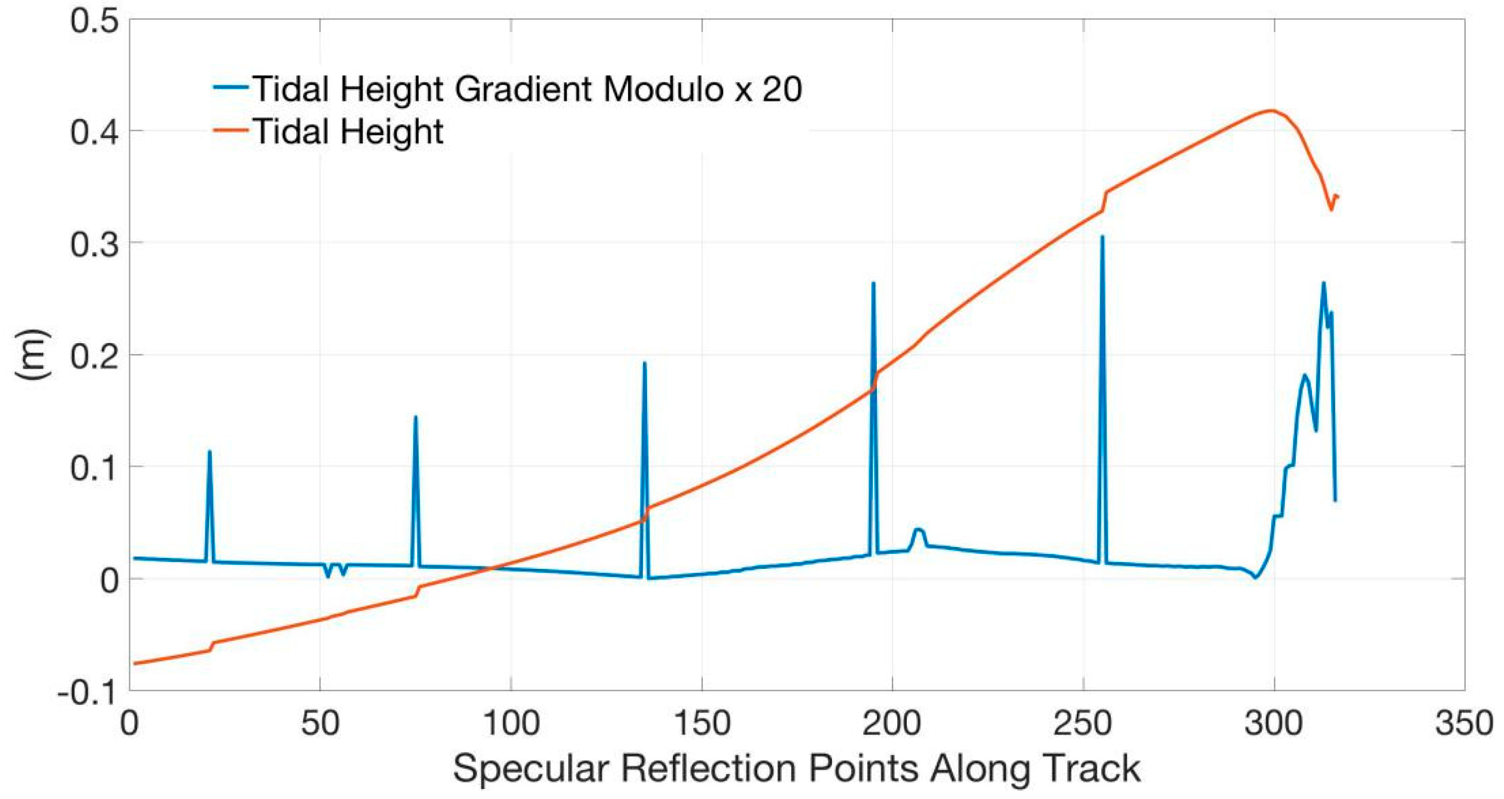
• The tidal height gradient and the corresponding tidal elevation position correction gradient of each track is calculated and detrended, the average is then subtracted, and the modulo is taken at last.
• Division of the offshore and the deep sea segments.
  Since some of the offshore tracks repeatedly cross land and sea, or cross islands, peninsulas, etc., one track is often divided into multiple sea sub-tracks by land, and the sub-tracks mostly contain offshore segments. Moreover, due to the complexity of the global coastline and tracks characteristics (length, direction, curvature, distribution, etc. [13]), the position of the offshore segment in the track is complicated. It could be divided into four cases: the offshore part is at one end of the track, at both ends of the track, in the middle of the track (the middle of the track is close to the land) or the entire segment is in the offshore (generally short tracks). The points where the tidal height gradient modulo in each track (or sub-track) are greater than 3 times the standard deviation η of the tidal height gradient modulo of the track are extracted. Then, the offshore and deep-sea segments are divided by these points according to the above four specific cases. Choosing too large a multiple of η would ignore some of the tidal height gradient points with sudden changes in the offshore, so that the offshore segment cannot be completely extracted. If the multiple is set too small, some high frequency peaks would be misjudged as offshore tidal height gradient mutation points. In addition, judging the continuous variation characteristics of the tidal height gradient requires the segment to be long enough, segments with more than 10 continuous points are selected.
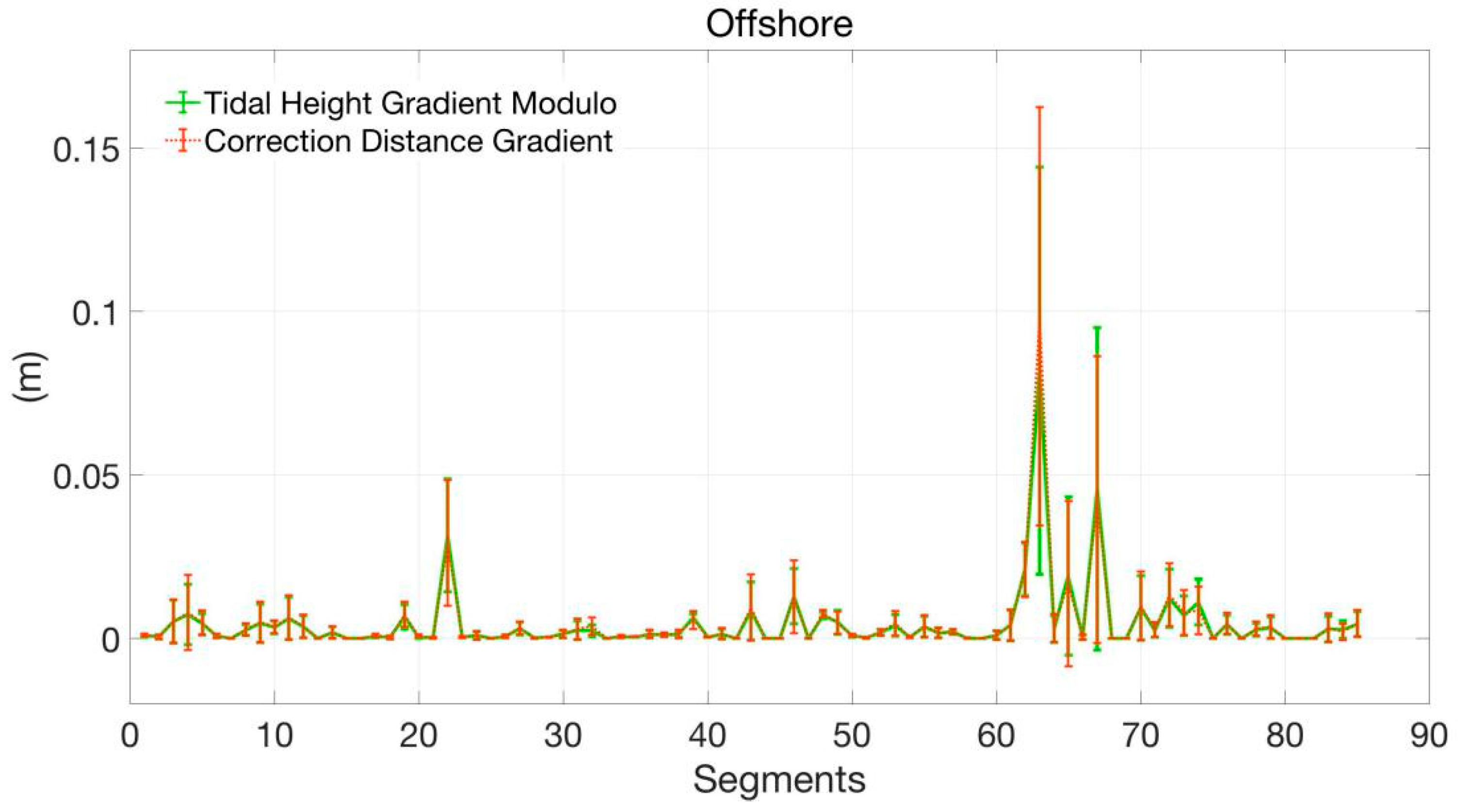
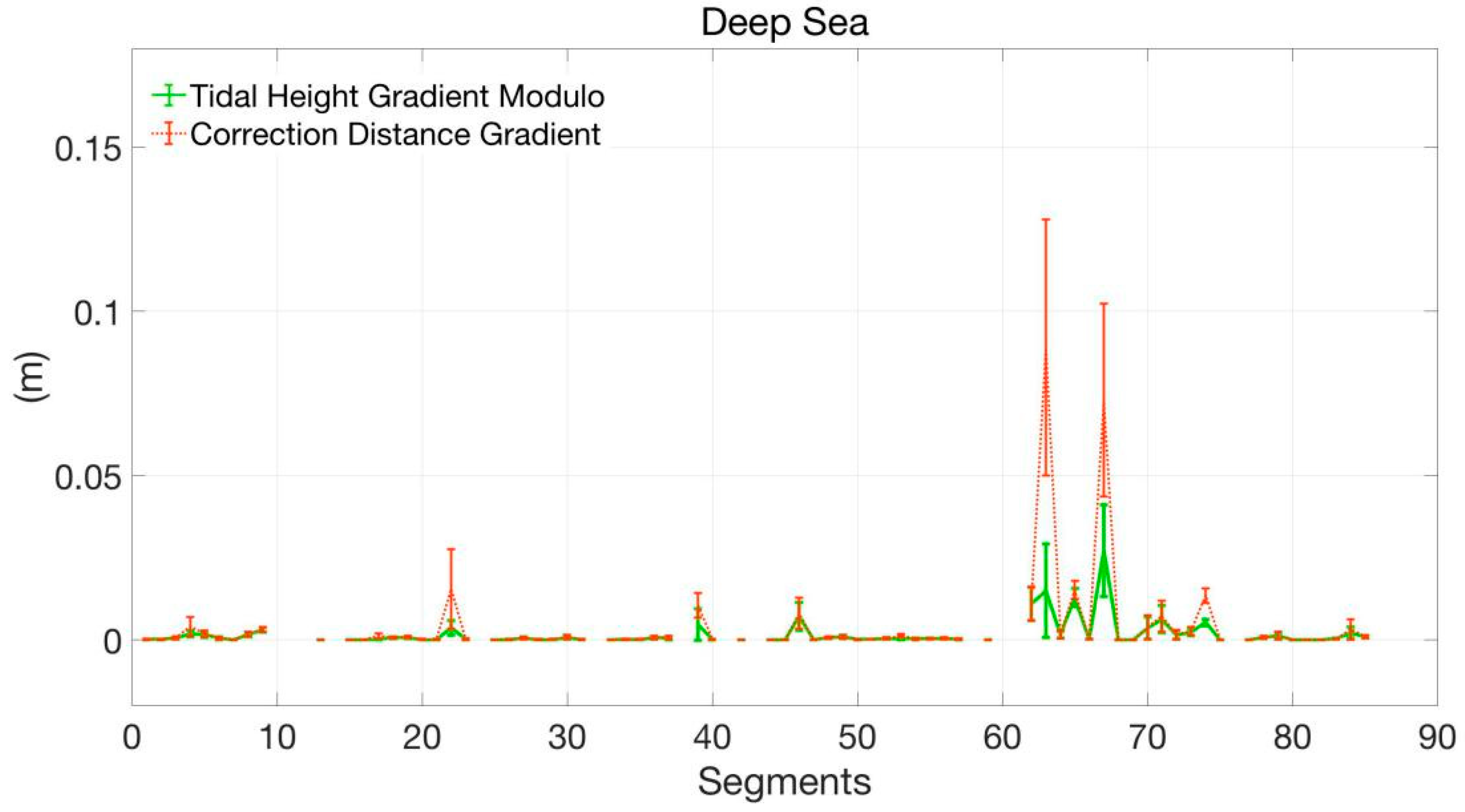
• Eliminating tidal height gradient jumping points.
  The points where the tidal height gradient modulo is greater than 3η in the deep sea segments are eliminated, and the tidal height gradient jumping peaks caused by the TDS-1 data jumping are well removed. According to the above filtering and division, 67 offshore segments are obtained, which contain 2476 specular reflection points, each segment has an average of about 37 points. And 54 deep sea segments are obtained, which contain 5716 specular reflection points, each with an average of approximately 106 points.

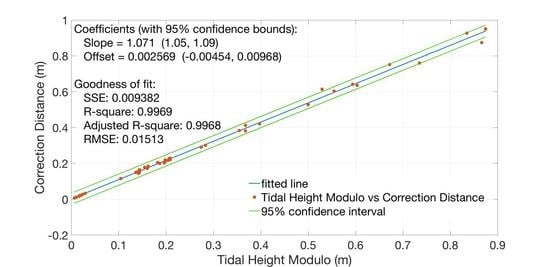
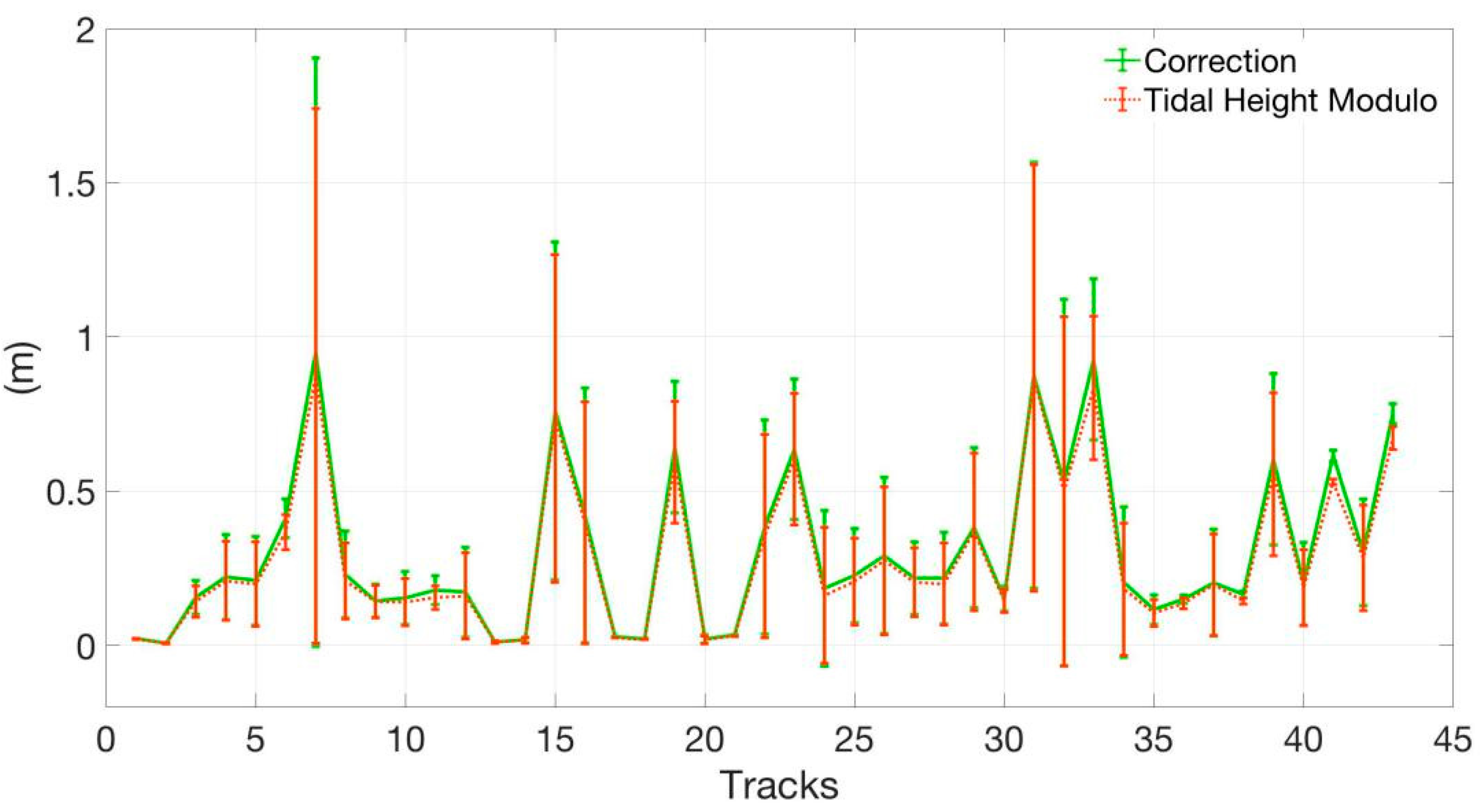
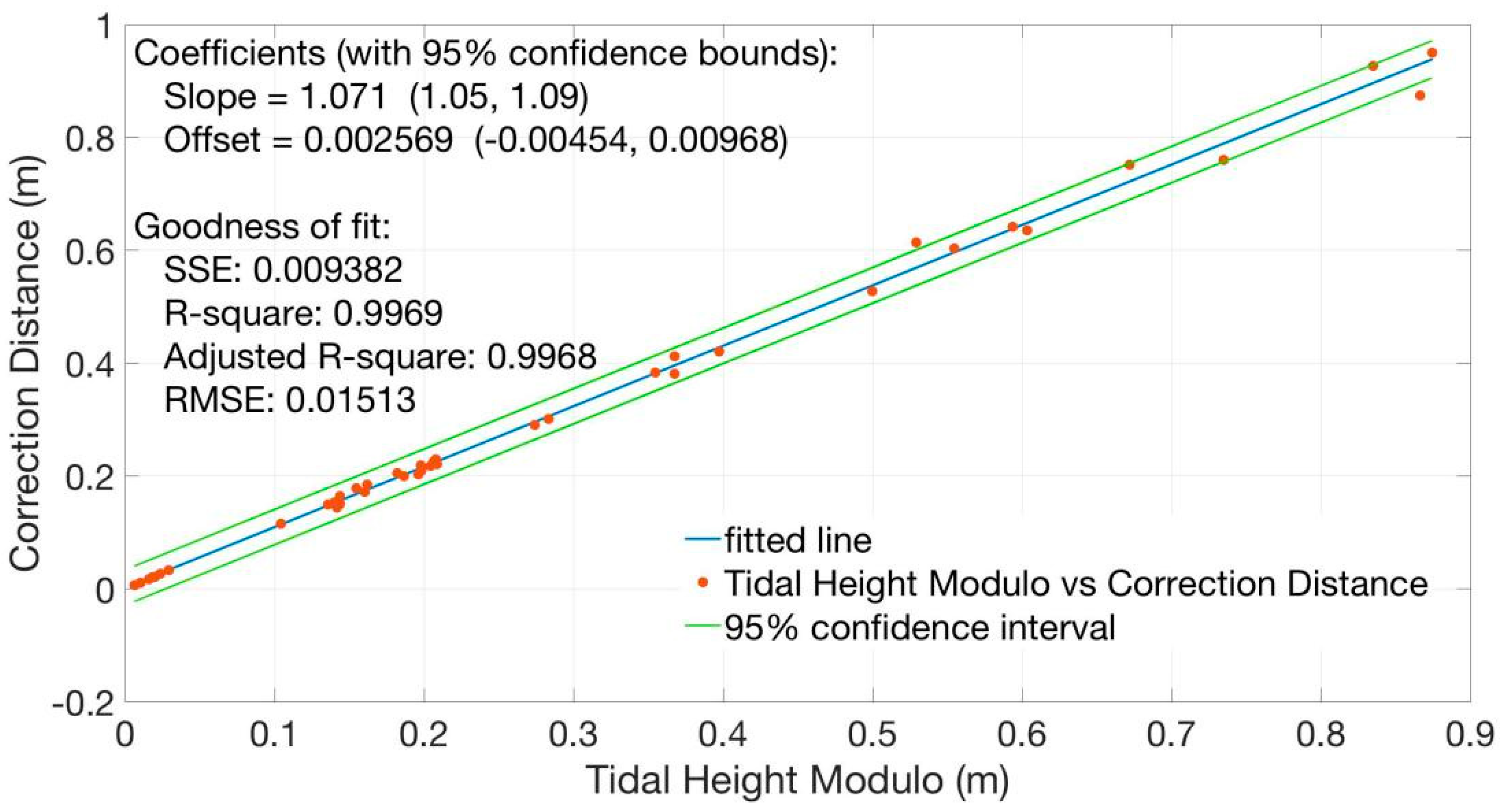
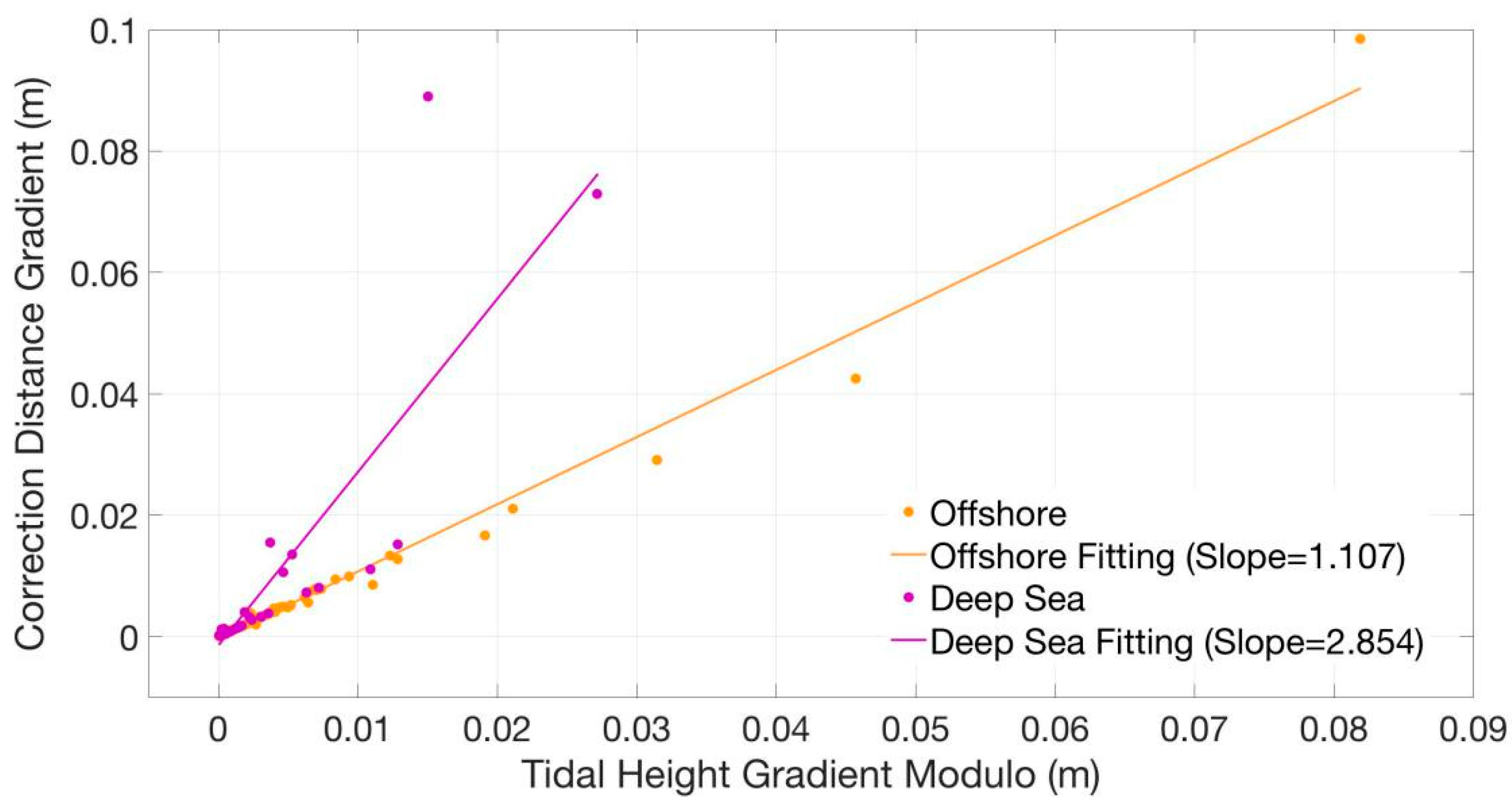
3.3. Tidal Height Gradient and the Tidal Positioning Correction Gradient

The average value and standard deviation of the tidal height gradient modulo and tidal correction gradient modulo of the offshore and deep sea segments are shown in

Table 2. Tidal height gradient modulo and the corresponding tidal positioning correction modulo of offshore and deep sea segments.

	Offshore		Deep Sea
	mean	std	mean	std
Tidal Height Gradient Modulo (m)	5.835 × 10−3	4.768 × 10−3	2.342 × 10−3	1.356 × 10−3
Correction Gradient Modulo (m)	6.122 × 10−3	5.023 × 10−3	5.267 × 10−3	2.417 × 10−3

, and those of each segment are shown in Figure 6, Figure 7 and Figure 8. The tidal height gradient modulo and its standard deviation in the offshore segments are significantly higher than those in the deep sea, with the gradient of about 2.5 times and the standard deviation of about 3.5 times. The tidal height change in the offshore is more dramatic than that in the deep sea, and the difference between segments (with different tidal amplitudes and phases) is greater. Compared with the large difference of the tidal height gradient modulo in the offshore and deep sea segments, the changes of the positioning correction gradient modulo in the two sea areas are closer. The correction gradient modulo in the offshore and its standard deviation are respectively 1.2 and 2 times those in the deep sea. The tidal height gradients modulo in the offshore segments have a positive correlation with the positioning correction gradient modulo. They are very close for all the segments, and the difference between them does not increase significantly with the increase of the gradient (see Figure 6 and Figure 8). This indicates that the variation of the tidal height in the offshore increases, and the change of the tidal correction is increased, the tidal positioning correction gradient modulo has a good response to the tidal height gradient modulo in the offshore. However, the difference between the two in the deep sea is larger, and the difference increases significantly with the increase of the gradient. The direct cause is that the gradient of the tidal positioning correction in the deep sea is higher than the tidal height gradient modulo; it does not decrease correspondingly as the tidal height gradient modulo decreases (see Figure 7 and Figure 8). It can be considered that the variation of the tidal positioning correction is more consistent with the tidal height gradient modulo in the offshore where the tidal height changes greatly. While the tidal height change tends to be gentle in the deep sea, the change of the tidal positioning correction does not greatly decrease with it. The sensitivity of the response of tidal positioning correction to the change of the tidal height is reduced in the deep sea compared to offshore. It is speculated that the change in terrain and gravity anomaly in the deep sea is more dramatic than in the offshore with the relatively flat continental shelf underwater, which makes the geoid undulation and the total elevation positioning correction change more in the deep sea [45]. This may contribute to the decreasing of the response sensitivity and the maintenance of high tidal correction gradient in the deep sea, which is consistent with the expression that the elevation positioning correction is affected by both gravity anomaly and tidal height in Section 2.2.

4. Conclusions

Based on the GNSS-R reflection reference surface elevation correction principle, this study uses the main parameters that determine the real-time variation of sea surface height, the ocean tide, to construct ocean tidal correction positioning method. The OTCP method is applied to correct the specular reflection point from geoid to the ocean tidal surface. The positioning error caused by the time-varying elevation difference of the reflection reference surface is reduced, the positioning based on the static-state elevation correction is improved. In addition, the different effects of the tides on the gradient of the tidal positioning accuracy improvement in the offshore and deep sea are discussed. According to the research results, the OTCP method improves the positioning by about 0.31 m relative to the geoid positioning. The improvement of positioning accuracy has a good correlation with the tidal height of different amplitudes and phases combinations. In the offshore, the tidal height gradient is larger than the deep sea, and the tidal positioning correction gradient modulo has a good response to the tidal height gradient modulo. In the deep sea, the sensitivity of the response decreases compared to the offshore.

References

1. Foti, G.; Gommenginger, C.; Jales, P.; Unwin, M.; Shaw, A.; Robertson, C.; Rosello, J. Spaceborne GNSS reflectometry for ocean winds: First results from the UK TechDemoSat-1 mission. Geophys. Res. Lett. 2015, 42, 5435–5441. [Google Scholar] [CrossRef] [Green Version]
2. Ruf, C.; Gleason, S.; Jelenak, Z.; Katzberg, S.; Ridley, A.; Rose, R.; Scherrer, J.; Zavorotny, V. The NASA EV-2 cyclone global navigation satellite system (CYGNSS) mission. In Proceedings of the 2013 IEEE Aerospace Conference, Big Sky, MT, USA, 2–9 March 2013; pp. 1–7. [Google Scholar]
3. Ruf, C.; Lyons, A.; Unwin, M.; Dickinson, J.; Rose, R.; Rose, D.; Vincent, M. CYGNSS: Enabling the future of hurricane prediction [remote sensing satellites]. IEEE Geosci. Remote Sens. Mag. 2013, 1, 52–67. [Google Scholar] [CrossRef]
4. Available online: http://www.cast.cn/Item/Show.asp?m=1&d=6544 (accessed on 5 June 2019).
5. Gleason, S.; Lowe, S.; Zavorotny, V. GNSS Applications Methods; Artech House: Boston, MA, USA, 2009; Volume 16, pp. 399–434. [Google Scholar]
6. Semmling, M. Altimetric Monitoring of Disko Bay using Interferometric GNSS Observations on L1 and L2. Ph.D. Thesis, Technical University of Berlin, Berlin, Germany, 2012. [Google Scholar]
7. Semmling, M.; Beckheinrich, J.; Wickert, J.; Beyerle, G.; Schön, S.; Fabra, F.; Pflug, H.; He, K.; Schwabe, J.; Scheinert, M. Sea surface topography retrieved from GNSS reflectometry phase data of the GEOHALO flight mission. Geophys. Res. Lett. 2014, 41, 954–960. [Google Scholar] [CrossRef] [Green Version]
8. Li, W.; Rius, A.; Fabra, F.; Martín-Neira, M.; Cardellach, E.; Ribó, S.; Yang, D. The impact of inter-modulation components on interferometric GNSS-Reflectometry. Remote Sens. 2016, 8, 1013. [Google Scholar] [CrossRef]
9. Li, W.; Cardellach, E.; Fabra, F.; Rius, A.; Ribó, S.; Martín-Neira, M. First spaceborne phase altimetry over sea ice using TechDemoSat-1 GNSS-R signals. Geophys. Res. Lett. 2017, 44, 8369–8376. [Google Scholar] [CrossRef]
10. Southwell, B.; Dempster, A. A new approach to determine the specular point of forward reflected gnss signals. IEEE J. Sel. Top. Appl. Earth Obs. Remote Sens. 2018, 11, 639–646. [Google Scholar] [CrossRef]
11. Li, W.; Rius, A.; Fabra, F.; Cardellach, E.; Ribo, S.; Martín-Neira, M. Revisiting the GNSS-R waveform statistics and its impact on altimetric retrievals. IEEE Trans. Geosci. Remote Sens. 2018, 56, 2854–2871. [Google Scholar] [CrossRef]
12. Li, W.; Cardellach, E.; Fabra, F.; Ribó, S.; Rius, A. Lake level and surface topography measured with spaceborne GNSS-Reflectometry from CYGNSS mission: Example for the lake qinghai. Geophys. Res. Lett. 2018, 45, 13–332. [Google Scholar] [CrossRef]
13. Wu, F.; Zheng, W.; Li, Z.; Liu, Z. Improving the GNSS-R Specular Reflection Point Positioning Accuracy Using the Gravity Field Normal Projection Reflection Reference Surface Combination Correction Method. Remote Sens. 2019, 11, 33. [Google Scholar] [CrossRef]
14. Helm, A. Ground-Based GPS Altimetry with the L1 OpenGPS Receiver Using Carrier Phase-Delay Observations of Reflected GPS Signals. Ph.D. Thesis, Postdam Deutsches GFZ, Potsdam, Germany, 2008. [Google Scholar]
15. Wu, S.-C.; Meechan, T.; Young, L. The potential use of GPS signals as ocean altimetry observation. In Proceedings of the National Technical Meeting, Santa Monica, CA, USA, 14–16 January 1997. [Google Scholar]
16. Yang, D.; Zhang, Q. GNSS Reflected Signal Processing: Fundamentals and Applications; Publishing House of Electronics Industry: Beijing, China, 2012. [Google Scholar]
17. Kostelecky, J.; Klokocnik, J.; Wagner, C.A. Geometry and acuracy of reflecting points in bistatic satelite altimetry. J. Geod. 2005, 79, 421–430. [Google Scholar] [CrossRef]
18. Beyerle, G.; Hocke, K. Observation and Simulation of Direct and Reflected GPS Signals in Radio Occultation Experiment. Geophys. Res. Lett. 2001, 28, 1895–1898. [Google Scholar] [CrossRef]
19. Rius, A.; Cardellach, E.; Martín-Neira, M. Altimetric Analysis of the Sea-Surface GPS-Reflected Signals. IEEE Trans. Geosci. Remote Sens. 2010, 48, 2119–2127. [Google Scholar] [CrossRef]
20. Skolnik, M. Radar Handbook; McGraw-Hill, Inc.: New York, NY, USA, 1990. [Google Scholar]
21. Gao, F.; Xu, T.; Wang, N.; Jiang, C.; Du, Y.; Nie, W.; Xu, G. Spatiotemporal Evaluation of GNSS-R Based on Future Fully Operational Global Multi-GNSS and Eight-LEO Constellations. Remote Sens. 2018, 10, 67. [Google Scholar] [CrossRef]
22. Jales, P.; Unwin, M. MERRByS Product Manual—GNSS Reflectometry on TDS-1 with the SGR-ReSI.; Surrey Satellite Technology LTD: Guildford, UK, 2017. [Google Scholar]
23. Liu, Y. Calibration Technology for HY-2 Radar Atimeter Sea Surface Height. Ph.D. Thesis, Ocean University of China, Qingdao, China, 2014. [Google Scholar]
24. Rosmorduc, V.; Benveniste, J.; Lauret, O.; Maheu, C.; Milagro, M.; Picot, N. Radar Altimetry Tutorial and Toolbox. 2011. Available online: http://www.altimetry.info (accessed on 20 May 2019).
25. Schwiderski, W. On charting global ocean tides. Rev. Geophys. 1980, 18, 243–268. [Google Scholar] [CrossRef]
26. LeProvost, C.; Genco, L.; Lyard, F. Spectroscopy of the world ocean tides from a finite element hydrodynamic model. J. Geophys. Res. Ocean. 1994, 99, 24777–24797. [Google Scholar] [CrossRef]
27. Cheng, Y.; Andersen, B. Multimission empirical ocean tide modeling for shallow waters and polar seas. J. Geophys. Res. Ocean. 2011, 116. [Google Scholar] [CrossRef] [Green Version]
28. Egbert, D.; Bennett, F.; Foreman, G. TOPEX/Poseidon tides estimated using a global inverse model. J. Geophys. Res. 1994, 99, 24821–24852. [Google Scholar] [CrossRef]
29. Egbert, D.; Ray, D. Significant dissipation of tidal energy in the deep ocean inferred from satellite altimeter data. Nature 2000, 405, 775–778. [Google Scholar] [CrossRef]
30. Egbert, D.; Erofeeva, Y. Efficient inverse modeling of barotropic ocean tides. J. Atmos. Ocean. Technol. 2002, 19, 183–204. [Google Scholar] [CrossRef]
31. Savcenko, R.; Bosch, W. E0TO8a–A New Global Tide Model from Multi—Mission Altimetry; Report No. 81; Deutsche Geodatisches Forschungsinstitut (DGFI): Mfinchen, Germany, 2008. [Google Scholar]
32. Ray, R.D. A Global Ocean Tide Model from TOPEX/Poseidon Altimetry: GOT99.2; NASA/TM-1999-209478; National Aeronautics and Space Administration, Goddard Space Flight Center: Greenbelt, MD, USA, 1999.
33. Murphy, C.; Moore, P.; Woodworth, P. Short-arc calibration of the TOPEX/Poseidon and ERS1 altimeters utilizing in situ data. J. Geophys. Res. 1996, 101, 14191–14200. [Google Scholar] [CrossRef]
34. Mitchum, G. Monitoring the Stability of Satellite Altimeters with Tide Gauge. J. Atmos. Ocean. Technol. 1998, 15, 721–730. [Google Scholar] [CrossRef]
35. Hwang, C.; Chen, S. Fourier and Wavelet Analyses of TOPEX/Poseidon-derived Sea Level Anomaly over the South China Sea: A Contribution to the South China Sea Monsoon Experiment. J. Geophys. Res. 2000, 105, 28785–28804. [Google Scholar] [CrossRef]
36. Rignot, E.; Padman, L.; MacAyeal, R.; Schmeltz, M. Observation of ocean tides below the Filchner and Ronne Ice Shelves, Antarctica, using synthetic aperture radar interferometry: Comparison with tide model predictions. J. Geophys. Res. Ocean. 2000, 105, 19615–19630. [Google Scholar] [CrossRef]
37. Dong, X.; Woodworth, P.; Moore, P.; Bingley, R. Absolute calibration of the TOPEX/Poseidon altimeters using UK tide gauges, GPS, and precise, local geoid-differences. Mar. Geod. 2002, 25, 189–204. [Google Scholar] [CrossRef]
38. Woodworth, P.; Moore, P.; Dong, X.; Bingley, R. Absolute calibration of the Jason-1 altimeter using UK tide gauges. Mar. Geod. 2004, 27, 95–106. [Google Scholar] [CrossRef]
39. Baltazar, A.O. Range and Geophysical Corrections in Coastal Regions: And Implications for Mean Sea Surface Determination, Volume Coastal Altimetry; Technical University of Denmark; Springer: Berlin/Heidelberg, Germany, 2011; pp. 103–146. ISBN 978-3-642-12795-3. [Google Scholar]
40. Liu, Y.; Tang, J.; Zhu, J.; Lin, M.; Zhai, W.; Chen, C. An improved method of absolute calibration to satellite altimeter: A case study in the Yellow Sea, China. Acta Oceanol. Sin. 2014, 33, 103–112. [Google Scholar] [CrossRef]
41. Pavlis, N.K.; Saleh, J. Error propagation with geographic specificity for very high degree geopotential models. In Gravity, Geoid and Space Missions; Jekeli, C., Bastos, L., Fernandes, J., Eds.; Springer: Berlin, Germany, 2005; p. 129. [Google Scholar]
42. Pavlis, N.K.; Holmes, S.A.; Kenyon, S.C.; Factor, J.K. The development and evaluation of the Earth Gravitational Model 2008 (EGM2008). J. Geophys. Res. Solid Earth 2012, 117. [Google Scholar] [CrossRef] [Green Version]
43. Bao, J.; Xu, J. Tide Analysis from Altimeter Data and the Establishment and Application of Tide Model; Surveying and Mapping Press: Beijing, China, 2013. [Google Scholar]
44. Lyard, F.; Lefevre, F.; Letellier, T.; Francis, O. Modelling the global ocean tides: Modern insights from FES2004. Ocean Dyn. 2006, 56, 394–415. [Google Scholar] [CrossRef]
45. Feng, S.; Li, F.; Li, S. Introduction to Ocean Science; Higher Education Press: Beijing, China, 2016. [Google Scholar]
Figure 1. GNSS-R reflection reference surfaces and the corresponding specular reflection points. Where S and S’ are the specular reflection points on geoid and ocean tidal surface, respectively. The purple arrow represents the positioning correction by the ocean tidal correction positioning (OTCP) method.
Remotesensing 11 01626 g001
Figure 2. The GNSS-R specular reflection point positioning geometry [13].
Remotesensing 11 01626 g002
Figure 3. Tidal height modulos and the corresponding tidal positioning corrections of the tracks.
Remotesensing 11 01626 g003
Figure 4. Tidal height modulos and the corresponding tidal positioning corrections of the tracks with the fitting of the two.
Remotesensing 11 01626 g004
Figure 5. Tidal height (red curve) and its gradient modulo (blue curve) of the specular points by the OTCP method on a deep sea-offshore track.
Remotesensing 11 01626 g005
Figure 6. Tidal height gradient modulos and the corresponding tidal positioning correction gradient modulos of the offshore segments.
Remotesensing 11 01626 g006
Figure 7. Tidal height gradient modulos and the corresponding tidal positioning correction gradient modulos of the deep sea segments.
Remotesensing 11 01626 g007
Figure 8. Tidal height gradient modulos, the corresponding tidal positioning correction gradient modulos and their fittings of the offshore and the deep sea segments.
Remotesensing 11 01626 g008