Article

Validation of Satellite, Reanalysis and RCM Data of Monthly Rainfall in Calabria (Southern Italy)

by
Giulio Nils Caroletti
1,
Roberto Coscarelli
1,* and
Tommaso Caloiero
2
1
National Research Council—Research Institute for Geo-Hydrological Protection (CNR-IRPI), 87036 Rende, Italy
2
National Research Council—Institute for Agricultural and Forest Systems in Mediterranean (CNR-ISAFOM), 87036 Rende, Italy
*
Author to whom correspondence should be addressed.
Remote Sens. 2019, 11(13), 1625; https://doi.org/10.3390/rs11131625
Submission received: 14 May 2019 / Revised: 2 July 2019 / Accepted: 3 July 2019 / Published: 9 July 2019

Abstract

:
Skills in reproducing monthly rainfall over Calabria (southern Italy) have been validated for the Climate Hazards group InfraRed Precipitation with Station data (CHIRPS) satellite data, the E-OBS dataset and 13 Global Climate Model-Regional Climate Model (GCM-RCM) combinations, belonging to the ENSEMBLES project output set. To this aim, 73 rainfall series for the period 1951–1980 and 79 series for the period 1981–2010 have been selected from the database managed by Multi-Risk Functional Centre of the Regional Agency for Environmental Protection (Regione Calabria). The relative mean and standard deviation errors, and the Pearson correlation coefficient have been used as validation metrics. Results showed that CHIRPS satellite data (available only for the 1981–2010 validation period) and RCMs based on the ECHAM5 Global Climate performed better both in mean error and standard deviation error compared to other datasets. Moreover, a slight appreciable improvement in performance for all ECHAM5-based models and for the E-OBS dataset has been observed in the 1981–2010 time-period. The whole validation-and-assessment procedure applied in this work is general and easily applicable where ground data and gridded data are available. This procedure might help scientists and policy makers to select among available datasets those best suited for further applications, even in regions with complex orography and an inadequate amount of representative stations.

Graphical Abstract

1. Introduction

Climate monitoring and analysis has received growing attention. Indeed, assessments have evidenced that temperature change over the last 50 years of the 20th century to a great extent results from anthropogenic forcings [1]. Observations are essential to climate monitoring since they are the basis for: (i) assessing century-scale trends; (ii) the validation of climate models; iii) the detection and attribution of changes in climate at regional scale. In particular, precipitation is a subject of special concern: since it is the main component of the global water cycle, it is also a major contributor to extreme events, and a crucial parameter in water resources management.
Precipitation observation is based primarily on ground rain gauges, then on weather radars and satellite retrievals. While rain gauges generally produce the most reliable observational results, they are often sparsely distributed; thus, they may not be fully representative of a region, especially for large areas with few observations [2]. In regions with complex orography and scarce human settlements, rain gauges are not enough to provide data to resolve precipitation processes in simulation studies. Satellite retrievals and climate reanalysis have thus been used to create regular data grids, in order to fill-in on lacking observations and to address the scarcity of stations in ungauged regions [3]. A climate reanalysis, combining model results with observations at regular grids, is often produced for every location on Earth, and spans a long time period that can extend back to several decades. Examples of climate reanalysis are: European Center Medium Weather Forecast’s (ECMWF) ERA-Interim [4], available at an horizontal grid of 80 km resolution from 1979 (and set to be replaced by the new ERA5); European Climate Assessment & Dataset project’s (ECAD) E-OBS, created by the ENSEMBLES (2004–2009, [5]) and further developed by the EUropean Reanalysis and Observations FOR Monitoring (EURO4M, 2010–2014, [6]) and Uncertainties in Ensembles of Regional ReAnalyses (UERRA, 2014–current, [7]) EU-funded projects, with European data from 1950 available on a 0.25° × 0.25° regular grid [8]; the various US National Centers for Environmental Prediction (NCEP) Climate Forecast System (CFS) products [9], available on a global scale since 1979 in various configurations with 0.5° to 2.5° spatial resolution.
Moreover, past data reconstructions are produced by climate models in control runs, for past periods that at least partly overlap with those with available observations and reanalysis. However, the matching of simulated and observed precipitation is especially difficult for Global Climate Models (GCMs), whose coarse grid cannot account for the horizontal variability detectable at small scales. Thus, various dynamical downscaling methods have been developed to refine large scale information by physical models. The most common approach to dynamical downscaling is the use of Regional Climate Models (RCMs) [10,11]. Various studies have recommended the use of as many models as possible when developing local climate change projections [12,13,14]. This approach has informed several EU-funded projects whose goal was to produce and assess multi-model and multi-scale datasets of climate change over Europe, i.e.: Prediction of Regional scenarios and Uncertainties for Defining EuropeaN Climate change risks and Effects (PRUDENCE, 2001–2004, [15]); Development of a European Multimodel Ensemble system for seasonal to inTERannual prediction (DEMETER, 2000-2003, [16]); the aforementioned ENSEMBLES [17]; Program for Climate Model Diagnosis and Intercomparison/Coupled Model Intercomparison Project—phase 3 (PCMDI/CMIP3, [18]); STAtistical and Regional dynamical Downscaling of EXtremes for European regions (STARDEX, [19]); and Climate Change and Variability: Impact on Central and Eastern Europe (CLAVIER, [20,21]).
Whatever the investigation method used, validation of precipitation’s large spatial and temporal variability is paramount and challenging at the same time [2]. Validation studies of control periods are routinely performed to monitor the performance of climate models, in order to evaluate their reliability in reproducing correctly the climatic properties of the studied area(s) [22,23]. For example, ENSEMBLES results were evaluated through the use of the E-OBS reanalysis dataset and further downscaled to a resolution of 1 km, as part of the activities of the EU FP-7 project CLimate Induced changes on the hydrology of the Mediterranean Basins (CLIMB, [24,25]).
Several satellite-based precipitation products have been evaluated on multiple spatial and temporal scales: for instance, Tropical Rainfall Measuring Mission’s Multi-satellite Precipitation Analysis (TRMM-MPA or TMPA); Climate Prediction Center morphing technique (CMORPH) precipitation; East Asian multi-satellite integrated precipitation (EMSIP); Precipitation Estimation from Remotely Sensed Information using Artificial Neural Networks (PERSIANN) [26,27,28,29]. The Climate Hazards group InfraRed Precipitation with Station data (CHIRPS) was developed to incorporate 0.05° resolution satellite imagery with in-situ station data to create gridded rainfall time series. CHIRPS is a quasi-global dataset spanning 50°S-50°N (and all longitudes), available from 1981 to the near-present. It has been evaluated in several countries, e.g., northern Italy [30], Cyprus [31], Brazil [32], Argentina [33], China [3], Eastern Africa (Ethiopia, Kenya and Tanzania [34]) and Mozambique [35]. CHIRPS was also among the best-performing datasets out of nine that were evaluated using hydrological modeling at 9053 catchments worldwide [36].
Metrics represent one of the most common tools in the assessment of data accuracy. Usually, defining generalized metrics is not possible, but they must be tailored: (i) on the specific use of the evaluated dataset; (ii) on the variable used; and (iii) on the regions of interest. To validate climate models via global precipitation measurements, Tapiador et al. [2] suggested the use of annual and seasonal comparisons, the analyses of bias and correlations, and the use of probability distribution functions as possible metrics. To evaluate skills in estimating and reproducing total monthly precipitation in CHIRPS, Funk et al. [37,38] and Toté et al. [35] used mean absolute errors and correlation coefficients for the Sahel, Afghanistan, south-western north America, Colombia, Mexico, Peru and Mozambique. Dembele and Zwart [39] studied the performance of seven gridded satellite rainfall products comparing them with data from nine weather stations in Burkina Faso. They used a point-to-pixel basis at various time steps (from daily to annual), using Pearson correlation coefficient, mean errors, bias, Root Mean Square Error (RMSE) and the Nash-Sutcliffe Efficiency coefficient.
Although rain gauges are most commonly used to validate datasets, the triple collocation (TC) technique has been increasingly used to characterize uncertainties in precipitation products, thanks to the availability of more and more datasets. This technique has been used to address problems arising from the validation of gridded data with a too coarse or sparse rain gauge network [40,41,42].
The goal of this study is to evaluate the skills of several datasets in reproducing monthly precipitation climatology. These sets include state-of-the-art reanalysis and satellite data, and well-tested model results, validated through an established and reliable rain gauge network. The study area is Calabria, a southern Italian region of about 15,000 km2. Calabria is a challenging area for rainfall studies: it has a complex orography and a high vulnerability to climate change due to its position in the center-south of the Mediterranean basin. At the same time, it is equipped with a robust rain gauge network, available through the Multi-Risk Functional Centre of the Regional Agency for Environmental Protection (Regione Calabria). For this study, CHIRPS has been used as the satellite dataset, E-OBS as the reanalysis dataset and 13 GCM-RCM combinations, available as outputs of the ENSEMBLES project, as the RC models. All these sets have been validated for the 1951–2010 time- period (CHIRPS only for 1981–2010) against the 79 rain gauges through (i) a two-metrics set consisting of adimensional, relative mean error and standard deviation error, and (ii) Pearson correlation.

2. Materials and Methods

2.1. Study Area

Located at the toe of the Italian peninsula, Calabria has a surface of 15,080 km2 and an average altitude of 597 m above sea level (a.s.l., hereafter).
With its tallest relief at 2266 m a.s.l., Calabria does not present many high peaks, yet it is one of the most mountainous areas in the country. Mountains (areas over 500 m a.s.l. high) occupy 42% of the region, while hills between 50 and 500 m a.s.l. high cover 49% of the territory. Only 9% of the region is under 50 m a.s.l. (Figure 1). Calabria’s climate is typically Mediterranean. It features sharp contrasts due to both its position within the Mediterranean Sea and to its orography. Specifically, warm air currents coming from Africa affect the Ionian side, leading to high temperatures, and to short and heavy precipitations. The Tyrrhenian side, instead, is affected by western air currents, which cause milder temperatures and more intense precipitations when compared to the Ionian side. Cold and snowy winters, and fresh summers with some precipitation, are typical of the inner areas of the region [43].

2.2. Data Sources

The following data sets have been validated:
  • The February 2019 update of CHIRPS (Climate Hazards group InfraRed Precipitation with Station data), version 2.0, with a 0.05° resolution and available from January 1981 until January 2019 [37];
  • The 18.0e version (released in November 2018) of E-OBS, a gridded version of the European Climate Assessment Dataset, with a 0.25° resolution and which provides data from January 1950 until June 2018 [8];
  • ENSEMBLES, funded by the European Commission’s 6th Framework Programme through contract GOCE-CT-2003-505539, consists of several GCM-RCM combinations, furnished at the E-OBS 0.25° grid [17]. These GCM-RCM combinations use a Global Climate Model (Table 1) to drive a Regional Climate Model (Table 2). As an example, the HCH-RCA acronym refers to the Sveriges Meteorologiska och Hydrologiska Institute (SMHI) regional RCA Model driven by the global Hadley Climate Model 3 (HCH) with high sensitivity. See Table 3 for a full list of GCM-RCM combinations and acronyms.
Several reasons determined the choice of the datasets:
  • CHIRPS and E-OBS are up-to-date, state-of-the-art products: they are regularly maintained and updated and they are the subject of several validation studies [44];
  • E-OBS has been used in previous studies as a validation tool for model outputs, and in particular to validate precipitation of the ENSEMBLES project GCM-RCM combinations [45,46,47];
  • the E-OBS fields are available on a grid consistent with that used by ENSEMBLES RCMs; in fact, they were technically built with the goal of direct comparison with ENSEMBLES RCM outputs [25,48];
  • ENSEMBLES models have already been selected and studied in previous projects; they are easily comparable with E-OBS, as they share the same spatial resolution and the same space grid; furthermore, they have data available for the 1951-2010 time-period.
The timeframe of the study goes from 1951 to 2010 in order to split the time period into two 30-years periods (1951–1980 and 1981–2010). This split allows to skill for the datasets from one 30-year period to another. In particular, the 1981–2010 time-period was chosen because it coincides with the current climatological normal period; moreover, CHIRPS data is available only from 1981 onward.
The validation has been conducted for monthly precipitation, because of its importance and relevance for research and for applications. First of all, it is used to build monthly normal climatology, which is a fundamental climatological parameter. It is also used: in calculating drought indices like Standard Precipitation Index (SPI; [49]); in evaluating rainfall seasonality, with, e.g., the Precipitation Concentration Index (PCI; [50]); in trying to understand the seasonal correlation between precipitation and teleconnections (e.g., El Nino Southern Oscillation, North Atlantic Oscillation); and runoff of monthly precipitation is also used as a driver of hydrological modeling (e.g., [51]). Finally, it must also be taken into account that many available datasets are only produced with monthly values, or restricted to monthly sampling (e.g., gauge-based precipitation products; see for instance [52]).
The validation set is based on daily data, available online, managed by the Multi-Risk Functional Centre of the Regional Agency for Environment Protection. The database consists of high quality and complete or near-complete records, available since early 20th century and currently updated. This set has been widely employed in the study of climate in Calabria (e.g., [53,54]). In particular, at the end of 2010, the Calabria database consisted of daily data collected at about 100 stations. All the rainfall series, which presented less than 80% of daily data in the observation period, were discarded. As a result, data from 79 stations in the period 1951–2010 (Figure 1 and Appendix A Table A1), with an average density of 1 station per 190 km2, were selected. Rain gauge density and distribution are crucial for an accurate description of rainfall amount over a region. It is difficult to derive fundamental laws to determine the gauge density needed in a particular region [55]. However, several studies proved a linear correlation between uncertainty in the spatially averaged rainfall and spatial standard deviation [56,57,58]. More recent theoretical developments suggest that uncertainty is directly proportional to the spatial standard deviation and inversely proportional to the square root of the total number of gauges [59]. World Meteorological Organization (WMO) guidelines indicated a number of stations per km2 ranging from one station per 100 km2 for complex, mountain terrain to one station per 10,000 km2 in arid and polar deserts [60]. Nonetheless, uncertainties are often calculated with different methods and metrics depending on the region of interest and the applications for which precipitation is needed (e.g., [61,62]). Mishra, for instance, suggested that for southern India the acceptable rain gauge density for reproducing significantly total precipitation was around 1 station per 350 km2 [61].
Small-scale variability influences rainfall events and monthly accumulated precipitation, so that validation at the smallest possible spatial scale is recommended. Interpolating gauge measurements into a gridded product results in large uncertainties [63]. Thus, for the CHIRPS versus observations comparison, we applied a point-to-pixel analysis which compared rainfall data observed at gauge stations with the respective grid cell; i.e., for each station and month, time series of data observed at selected rain gauges were compared to the corresponding CHIRPS pixel [36,64].
In comparing gauge measurements and E-OBS/ENSEMBLES grid points, grid data were interpolated to the station location and we compared the results to the station data. Numerous studies have provided reviews of existing spatial interpolation methods for hydrological variables (e.g., [65]) or suggested new spatial interpolation approaches (e.g., [66]). Among these studies, there was not a unanimous consensus on the best interpolation method: several authors have concluded that results depend on the sampling density (e.g., [67]). A bilinear interpolation has been chosen because it is a simple, two-dimensional (2D) interpolation and it allows to perform a clear assessment of improvements and uncertainties introduced.

2.3. Validation Metrics

Different metrics can evaluate different skills in reproducing precipitation. For this study, three common evaluation metrics were used: the relative mean error, the relative standard deviation error, and the Pearson correlation coefficient [2,25,36].
These metrics have been selected for the following reasons:
  • Mean error and standard deviation error are among the most commonly used tools in validation and error theory [68,69], and also to compare E-OBS and ENSEMBLES RCMs [25];
  • The Pearson correlation coefficient is an important measure commonly used in climate science for evaluating data from independent data sources, just like precipitation values from gauge stations, satellites and models [70,71].
The use of mean error and standard deviation assume that the error distribution is Gaussian. We checked preliminarily that monthly precipitation data over Calabria followed roughly a normal distribution for rain gauge data, E-OBS and CHIRPS. It is then a common assumption that the errors are normally distributed as well (e.g., Roebeling et al. [40]).
It is interesting to note that the approximately normal distribution of E-OBS, CHIRPS and of the gauge network, three independent sets with mutually uncorrelated errors, might satisfy the requirements for applying triple collocation validation. However, the mutual independence of the sets might be only apparent, as both E-OBS and (partially) CHIRPS are built using rain gauge data. Thus, more preliminary analyses are needed before using triple collocation to assess the performance of these sets.
There are many other methods and indices that can be used; however, many of these are not independent of mean and standard deviation, or are basically different methods to calculate correlation. Others, such as the number of rainy days, could not be used as we do not have daily data for most of these sets.

2.3.1. Mean Error and Standard Deviation Error

The two-metric validation introduced in this section is based on the work of Deidda et al. [25]. They used it to evaluate ENSEMBLES RCMs’ skills in reproducing precipitation (and temperature) against E-OBS reanalysis data. The performance indices are the monthly mean and standard deviation adimensional errors. The mean error evaluates how well the estimates correspond to the observed values, indicating whether rainfall totals are overestimated or underestimated. The standard deviation evaluates the average magnitude of estimated errors, and the capability at reproducing variability.
Let PS (m, y) be monthly precipitation, for month m, year y and for a generic dataset s that we want to validate. It can be collected at a station, a grid point, or as an averaged value over an area (e.g., a hydrological basin or an administrative district).
Considering a climatological time-frame that takes into account a number Ny of years of monthly averaged precipitation PS (m, y), starting with year y0, the Ny-years average of the monthly precipitation for each month in the annual cycle μs(m) is:
μ s ( m ) = 1 N y y = y 0 y 0 + N y 1 P s ( m , y ) ,
and the standard deviation of precipitation of month m is:
σ s ( m ) = 1 N y 1 y = y 0 y 0 + N y 1 | P s ( m , y ) μ s ( m ) | 2 .
Each dataset has to be compared with the observed data (registered in the rain gauges). Just like in Equation (1) and Equation (2), it is possible to estimate, also for the observed dataset, the Ny-years average of the monthly precipitation P0 (m, y):
μ 0 ( m ) = 1 N y y = y 0 y 0 + N y 1 P 0 ( m , y ) ,
and the standard deviation:
σ 0 ( m ) = 1 N y 1 y = y 0 y 0 + N y 1 | P 0 ( m , y ) μ 0 ( m ) | 2 .
Within this aim, the following error metrics have been introduced:
a) The average absolute error on the monthly mean:
E μ s = 1 12 m = 1 12 | μ s ( m ) μ 0 ( m ) | ;
b) The average absolute error on the standard deviation:
E σ s = 1 12 m = 1 12 | σ s ( m ) σ 0 ( m ) | .
The above defined error metrics provide information on the reliability of a single model in reproducing precipitation, whereas normalizing metrics is needed to visualize more clearly the simultaneous performance of different datasets against each other.
To produce normalized metrics for datasets, each error has been divided by a factor obtained as the sum of errors on all datasets (S):
f μ = s = 1 S E μ s ,
f σ = s = 1 S E σ s .
The errors on the climatological mean of a single dataset become:
ε μ s = E μ s f μ ;
ε σ s = E σ s f σ .
The results can be graphically represented in a simply Cartesian plane, by drawing the mean error and the standard deviation error on the x- and y-axes, respectively. The origin (0,0) indicates the reference value. The closest the error metrics for a dataset s are to the origin, the better its performance.
This procedure can be easily generalized from a two-dimensional error to a N-dimensional error by including any relative indices relevant to the specific study. It might even be possible to provide every index with a weighting factor. The use of more and/or different indices would be up to the specific scientific problem’s demands.
As the absolute standard deviation represents the degree of dispersion, Equation (6) can be used as a bias error estimate (see [72,73]). On the other hand, while the relative bias error is defined as the bias error divided by the mean precipitation, Equation (10)’s relative error is normalized over the errors of all other models. Thus, this error measure is not a relative bias index.

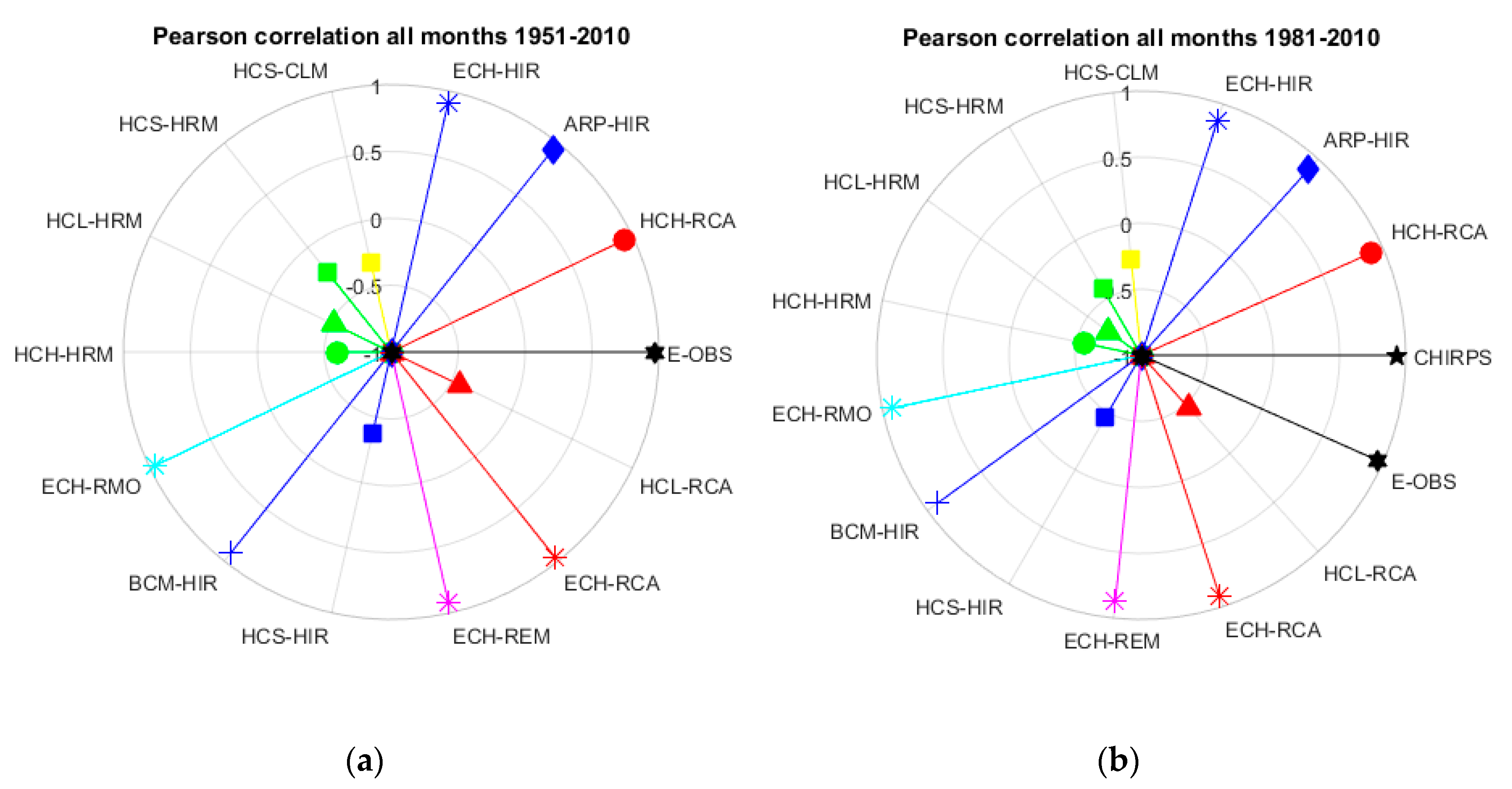
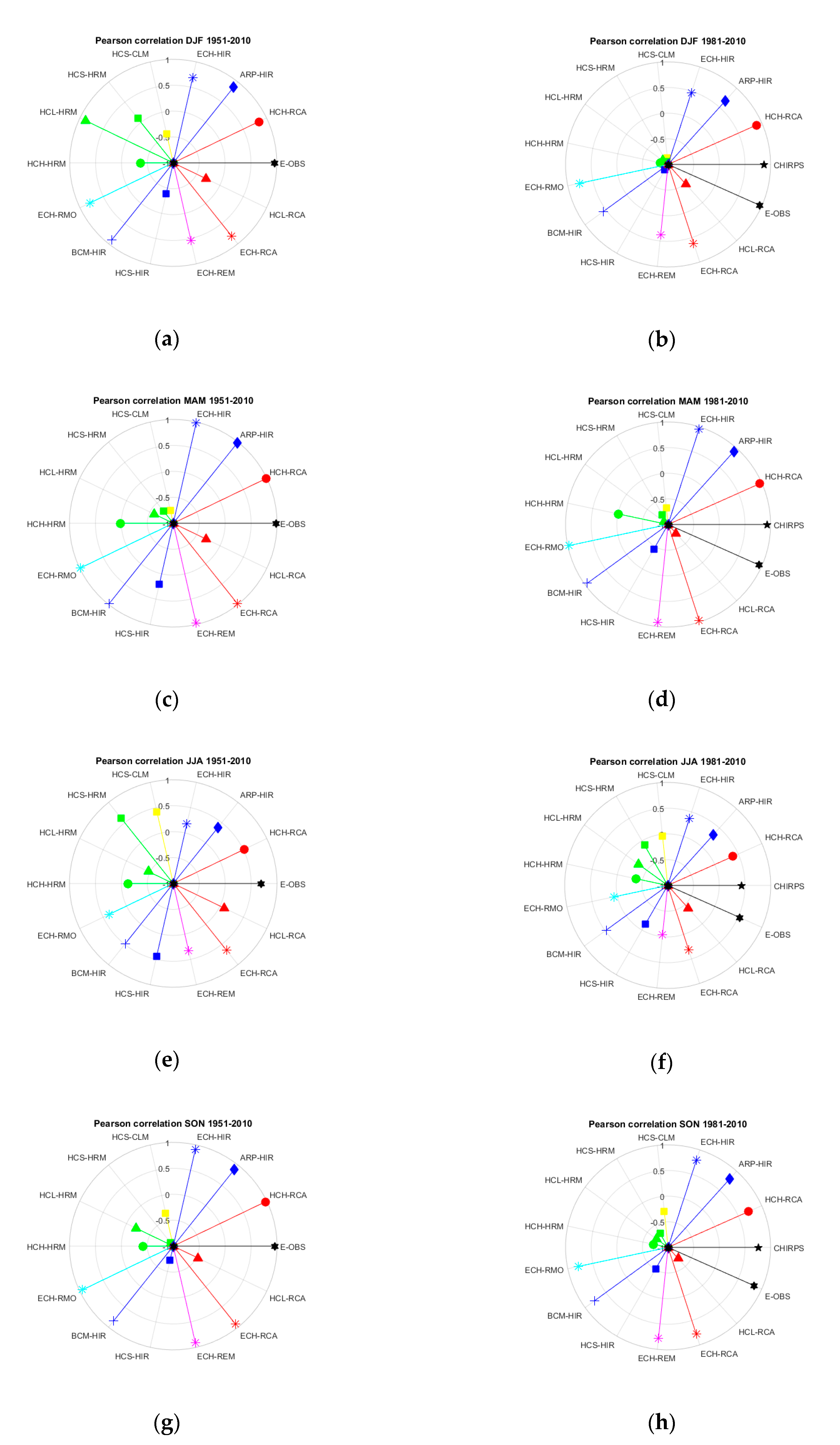
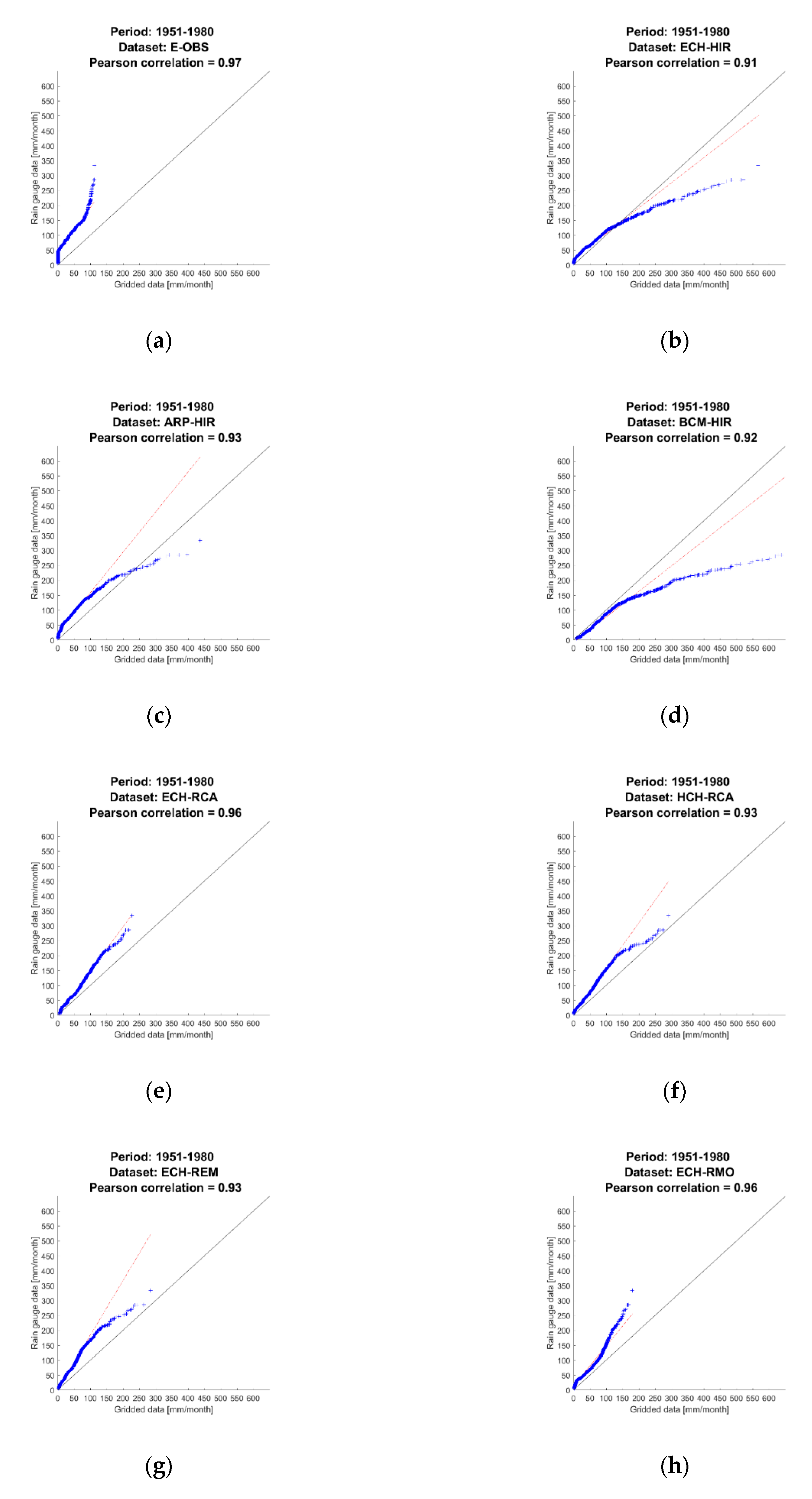
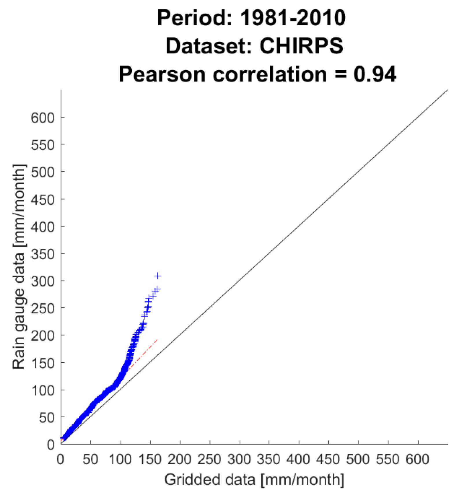
2.3.2. Pearson Correlation Coefficient

The Pearson correlation coefficient (r) has been used to evaluate how well the estimates corresponded to the observed values. For each month (m) and each dataset (s), the coefficient is defined as:
R ( m , s ) = y = 1 N y [ P 0 ( m , y ) μ 0 ( m ) ] [ P s ( m , y ) μ s ( m ) ] y = 1 N y [ P 0 ( m , y ) μ 0 ( m ) ] 2 y = 1 N y [ P s ( m , y ) μ s ( m ) ] 2 ,
with values ranging from −1 to 1 with the extremes ±1 indicating the perfect scores [70,71,74].
Ny indicates the number of years taken into account, i.e., 30 or 60 (except for CHIRPS, for which Ny = 30 only).

3. Results

Results from the adimensional mean-and-standard deviation metrics (Figure 2) showed that some model results from ENSEMBLES compare well with satellite data (CHIRPS) and reanalysis tools (E-OBS).
In particular, CHIRPS and the four ECHAM5-driven models are the best performers overall, both in terms of standard deviation and mean. From the other ENSEMBLES combinations, good relative performances were obtained by HCH-RCA and ARP-HIR.
There is very little change in relative performance between the two considered time periods, with the exception of E-OBS and of the ECHAM5-driven models. In particular, all of the latter models increase their relative skills in reproducing standard deviation; and three out of four increase the skills in the mean from the 1951–1980 to the 1981–2010 time-period (Figure 3).
The noticeable improvement in E-OBS relative results (Figure 2b) is probably due to the addition of new stations and observations to the dataset used for the reanalysis.
Figure 4 shows the Pearson correlation coefficient, evaluated between monthly rain gauge precipitation and gridded dataset precipitation, for the whole observation period (1951–2010) and for the 1981–2010 time period only. The correlation shows that the same models that had good relative error metrics are the best-performing ones (ECH-driven models, HCH-RCA and ARP-HIR), with the addition of BCM-HIR. However, the most correlated dataset of all (r = 0.97) is E-OBS, which was only an average performer with regard to relative metrics. CHIRPS is once again an excellent performer, with a correlation value of r = 0.94.
The other six models (all driven by the Hadley Center HadCM3 Model) score very bad on the Pearson correlation. They all show anticorrelation, with values ranging from r = −0.23 (HCS-HRM) to r = −0.59 (HCH-HRM), which means that it is not possible to identify any linear relation between the model data and the rain gauge data.
A huge difference between the results obtained from two regional models driven by the Hadley Model with high sensitivity has been detected: HCH-RCA is one of the best performers at all metrics, while HCH-HRM is one of the worst.
Figure 5 shows the seasonal correlation of monthly rain gauge precipitation with gridded dataset precipitation. The seasonal breakdowns show a good performance of nine datasets in the spring (MAM) and in the fall months (SON). The E-OBS is the only dataset with an excellent correlation (r > 0.9) in the winter months (DJF), while all datasets show a strong decrease in correlation for the summer months.
The six anticorrelating models show a wildly inconsistent behavior from season to season and from 1951–1980 to 1981–2010. For example, HCL-HRM (r = −0.52 for all months in the 1951–2010 time period) has a correlation value r = +0.92 in the winter months for the 1951–1980 time period (not shown in figures), and r = −0.87 if we consider the 1981–2010 time period, with seasonal values for the 1951–2010 period varying from r = +0.87 in winter to r = −0.59 for spring.
To further understand the strengths and weaknesses of the examined datasets in reproducing precipitation features in Calabria, we have examined Quantile-Quantile plots (QQ-plots) of monthly precipitations of all stations for each dataset. Figure 6 shows the QQ-plots of gridded data against station data for the full 1951–2010 time period, for E-OBS and the seven best-correlating (r > 0.9) models from ENSEMBLES. Figure 7 shows the results for 1981–2010 for CHIRPS.
Results from QQ-plots and relative metrics show how E-OBS is not one of the best models. However, it must be noted that it still correlates very well with the observed data. From the plots, it is clear that most of the well-performing models have good or even excellent results at the lower spectrum of the precipitation range. However, they are not able to reproduce correctly the months with most precipitation. This is probably due to a lack of skill in reproducing extreme events (for models) or problems in satellites in observing them (TRMM). It is possible that this problem is transferred from raw satellite data to methods that integrate satellites with stations (CHIRPS) or use satellite data in reanalysis (E-OBS).
Analogous QQ-plots (not shown) were examined for the full 1951-2010 time period for the seven mildly anticorrelating (−0.53 < r < −0.23) models from ENSEMBLES. It is clear that the gridded data here do not follow any recognizable linear pattern for a long enough interval to allow some form of linear correlation to emerge.

4. Discussion

Results from this study show the importance of using multiple metrics in validation: combining the analysis from several tools provides a deeper understanding of the datasets’ skills and shortcomings.
The relative error metrics show which datasets perform better as to what concerns actual monthly precipitation values. However, Pearson correlation is also an important validation tool: a high correlation (i.e., correlation values above 0.8) means that it might be possible to obtain better results with a simple bias correction. For example, we could use the Pearson value to select only high-correlating datasets, then bias-correct them (for instance, with a simple linear regression), and finally re-run the relative metrics to find the best-performing models. In general, however, one must always remember that metrics should be tailored on the desired end-use of the datasets: metrics are not a measure of quality per se.
Bias correction, for instance, might be useful with the E-OBS data: while this reanalysis gridded set shows the highest correlation values (r = 0.97), its performance is only average with respect to the relative, normalized error metrics. E-OBS shows a strong tendency to underestimate precipitation amounts in general and extreme events in particular. The mean yearly precipitation for 1951–2010 is 1057 mm/year according to the observations, while it is only 606 mm/year according to E-OBS (see Appendix A and Table A1 for more information on the datasets’ mean yearly precipitation). This underestimation has also been found in other studies that have shown a bias in E-OBS toward lower values [44].
With regard to possible bias corrections, it must be noted that the ENSEMBLES models have associated the available elevation data, which can be used for vertical corrections. On the other hand, CHIRPS precipitation is based on satellite data, and has no orographic reference. Caroletti and Deidda [75] applied bias correction and orographic correction to downscale precipitation of 14 ENSEMBLES models in Sardinia. They improved the skill in reproducing results, using a combination of a multifractal model and of a linear orographic model. This could be usefully applied to the mountainous regions of western Calabria, where precipitation has a strong orographic component. However, this method would not solve the issue concerning months with high amounts of convective precipitation.
Balsamo et al. suggested spatial re-scaling as a way to improve gridded dataset results [66]. The main problem for Calabria would be to find a reliable gridded reference to use for re-scaling. An alternative approach could be the spatial interpolation of the rain gauge network into a regular-spaced grid.
E-OBS could be considered a reliable enough dataset for this purpose. However, E-OBS is provided at the same grid (and space resolution) as ENSEMBLES, so there would not really be a re-scaling. Even though E-OBS could be used to re-scale CHIRPS data, more problems could come from re-scaling satellite data at cell level into a point-grid system (see Section 2.2). Another choice of dataset could be ERA-INTERIM, which has a resolution of about 80 km, but is only available from 1979 to 2017 [76,77].
With regard to the interpolation of the rain gauge network to a regular grid, one of the main issues would be what method to use for building the grid. Several tools are available for sparse data interpolation: the Barnes method, for instance, has been used successfully for precipitation [25]. The problem of rescaling cell data to grid points, though, would still have to be addressed.
CHIRPS has a very high correlation value (0.94) and a high relative error skill compared to other models. This dataset seems to be an excellent basis for further work, especially given the fact that it has a 0.05° resolution compared to the 0.25° resolution of all other datasets taken into account. Precipitation estimates derived from satellite data are indirect and are inevitably accompanied by a large degree of variability, and have difficulty representing precipitation with high spatiotemporal variability in areas of complex topography [52,78]. CHIRPS results, however, show no particular problem in capturing light precipitation. This is probably due to the incorporation of station data in satellite products.
Good Pearson correlation results and an underestimation of high precipitation events were in accord with previous evaluations: Paredes-Trejo et al. [32] in northeast Brazil, and Luo et al. [79] in the Lancang-Mekong river basin, where they used CHIRPS data to drive hydrological modeling. On the other hand, Rivera et al. [33] noted some issues in the Andes region of Argentina, where CHIRPS underperformed especially in areas above 1000 m a.s.l. As there are only a handful of stations located above that altitude in this study, this begs for some caution in the use of the CHIRPS dataset. This is especially noteworthy given the importance of mountain areas of Calabria as the main freshwater sources for the region. Bai et al. [3] investigated the performance of CHIRPS over China, finding very different results in different regional and basin areas, wet versus arid zones, and summer versus winter months. Once again, this underlines the importance of taking case region validations as valid only for that specific region and for the specific use the data is validated and selected for.
Deidda et al. [25] used E-OBS to validate 14 ENSEMBLES models. However, although the Pearson correlation with ground data is excellent, the relative error metrics show that some of the ENSEMBLES models perform better than E-OBS. Since the ENSEMBLES models are built at least in part on the E-OBS results, this is not necessarily surprising. However, this might question the idea of using E-OBS as a validation method for these models, as ENSEMBLES and E-OBS are not independent of each other.
In general, Pearson correlation results show huge problems in reproducing summer precipitation. However, this has a lesser impact on the relative error metrics, as they are based on the sum of all errors on the monthly means; thus, the contribution to the error from summer months is much reduced, as summer precipitations in Calabria are significantly less than precipitation during the other months of the year.
Poor summer performance, on the other hand, might contribute to errors in extreme events evaluation for E-OBS and CHIRPS, as extreme events can affect Calabria in the form of late summer thunderstorms and extreme convective precipitation.
The reliability of RCMs in general is strongly dependent on the quality of the climate forcing data, i.e., of the GCMs. It is plausible that the ECH-driven models are the best performers in general because of the quality of their forcing data, which is more important than the RCMs fine-tuning. The three models driven by the Hadley Centre HadRM3Q3 Model (HCL-HRM, HCS-HRM and HCH-HRM), are better during 1951–2010 than 1981–2010 according to the Pearson correlation coefficient. By looking at the seasonal correlations, we see that the performance is almost the same in the spring season, while it worsened for the other seasons; most significantly, it worsened for winter months, where it went from a good correlation to anti-correlation. In the 1981-2010 time period, there was an increase in extreme precipitation and a decrease in the number of precipitation days in Calabria [80], especially in winter [81]. This change in precipitation patterns might have escaped the HRM climatology that drove these RCMs; even though the 30-years climatology of precipitation (i.e., the decrease of the yearly average) might have been correctly reproduced (see Appendix A Table A2).
The performance of RCMs in regard to extreme events, on the other hand, depends on the skill of the regional model to capture correctly spatial distribution of precipitation and orographic enhancing. In this regard, we found that RCA regional models were the best performers: even HCL-RCA, which is one of the lower ranking datasets overall, actually correlates more at extreme events than for all the rest of the precipitation spectrum (not shown). Results from ENSEMBLES models run with the HIRHAM5 RCM, show the opposite problem: even those with good correlation values, strongly overestimate extreme events. Thus, it is not surprising that BCM-HIR and ECH-HIR are the datasets with the highest yearly precipitation values (see Appendix A Table A2).

5. Conclusions

Products distributed on regular grids, whether satellite data, reanalysis products, or model data, are currently used for most climatological studies, especially in regions where ground stations are inadequate to perform high-resolution regional studies. A common approach in future projections studies is to produce large ensembles of climate model results. Many studies (e.g., [13] and [14]) suggest that the results from all available models are used to span the uncertainties coming from different approaches (e.g., on parameterizations). However, other studies [22,69,82] challenge this approach and suggest weighting the models contribution, or using a limited number of high-performing model results instead. The selection of the most accurate gridded products—i.e., validation—can play a major role in accurate climate projections, assessment studies and hydrological studies.
The results of this study showed that, taking into account Pearson correlation, error metrics and extreme events performance, the best datasets are the satellite-based CHIRPS dataset and the ECH-RCA, HCH-RCA and ECH-REM models from the ENSEMBLES set. Given its high correlation values, E-OBS data could be a good dataset to use for further applications, but only after bias correction. There was a slight appreciable improvement in performance for all four ECHAM5-based models and for the E-OBS dataset from the 1951–1980 to the 1981–2010 time-period.
Results from this validation show that, out of 13 ENSEMBLES models, the ones with the worse error metrics are also the ones of which the monthly precipitation data do not correlate with rain gauge data. Thus, to calculate ensemble uncertainties using models showing these performances might be in fact counterproductive.
The whole validation procedure presented in this study is general and easily applicable to any other region where ground- and gridded-data are available, as a supporting tool in the choice of data for precipitation assessments in areas with sparse ground data.

Author Contributions

Conceptualization, C.G.N. and C.R.; methodology, C.G.N.; software, C.G.N. and C.T.; formal analysis, C.G.N. and C.T.; validation: C.T. and C.R.; investigation, C.G.N.; data curation, C.R. and C.T.; writing—original draft preparation, C.G.N.; writing—review and editing, C.R. and C.T.; visualization, C.G.N. and C.T.; supervision, C.R.; project administration, C.R.

Funding

This research was funded by FORMAS (SE), DLR (DE), BMWFW (AT), IFD (DK), MINECO (ES), ANR (FR) with co-funding by the European Union, Grant number 690462

Acknowledgments

The Project INDECIS is part of ERA4CS, an ERA-NET initiated by JPI Climate, and funded by FORMAS (SE), DLR (DE), BMWFW (AT), IFD (DK), MINECO (ES), ANR (FR) with co-funding by the European Union (Grant 690462).

Conflicts of Interest

The authors declare no conflict of interest.

Appendix A

This Appendix shows the rain gauges of the Multi-Risk Functional Centre used for the validation (Table A1), and yearly mean precipitation results from the two time series for all validated datasets and for the validation data (Table A2), averaged over all available stations for that time period and that dataset.
Table A1. Rain gauges of the Multi-Risk Functional Centre of the Regional Agency for Environmental Protection, with code number and station name.
CodeNameCodeName
900Albidona2090Fabrizia
930Villapiana Scalo2130Roccella Ionica
970Cassano allo Ionio2150Fabrizia - Cassari
1000Domanico2160Gioiosa Ionica
1010Cosenza2200Antonimina
1030San Pietro in Guarano2210Ardore Superiore
1060Montalto Uffugo2230Plati’
1092Camigliatello – Monte Curcio2260San Luca
1100Cecita2270Sant’Agata del Bianco
1120Acri2290Staiti
1130Torano Scalo2310Capo Spartivento
1140Tarsia2320Bova Superiore
1180Castrovillari2340Roccaforte del Greco
1230San Sosti2380Montebello Ionico
1360Longobucco2450Reggio Calabria
1380Cropalati2510Scilla
1410Cariati Marina2540Santa Cristina d’Aspromonte
1440Crucoli2560Sinopoli
1455Ciro’ Marina - Punta Alice2580Molochio
1500Nocelle - Arvo2600Cittanova
1580Cerenzia2610Rizziconi
1670Cutro2670Arena
1675Crotone - Papanice2690Feroleto della Chiesa
1680Crotone2710Mammola - Limina C.C.
1695Crotone - Salica2730Mileto
1700Isola di Capo Rizzuto - Campolongo2740Rosarno
1740San Mauro Marchesato2760Joppolo
1760Botricello2780Zungri
1780Cropani2800Vibo Valentia
1820Soveria Simeri2830Filadelfia
1830Albi2890Tiriolo
1850Catanzaro2940Nicastro - Bella
1910Gimigliano2990Parenti
1940Palermiti3000Rogliano
1960Chiaravalle Centrale3040Amantea
1970Soverato Marina3060Paola
1980Serra San Bruno3090Cetraro Superiore
2040Monasterace - Punta Stilo3100Belvedere Marittimo
2086Mongiana3150Laino Borgo
3160Campotenese
Table A2. ENSEMBLES Regional Climate Models used in the CLIMB validation.
Dataset1951–1980 (mm/year)1981–2010 (mm/year)
HCH-RCA748716
ARP-HIR723648
ECH-HIR11461076
HCS-CLM810777
HCS-HRM746681
HCL-HRM550471
HCH-HRM783763
ECH-RMO733733
BCM-HIR15861485
HCS-HIR12171179
ECH-REM672662
ECH-RCA777744
HCL-RCA904790
E-OBS617596
CHIRPS-766
Gauge data1128986

References

  1. IPCC. Climate Change 2013: The Physical Science Basis. Contribution of Working Group I to the Fifth Assessment Report of the Intergovernmental Panel on Climate Change; Stocker, T.F., Qin, D., Plattner, G.-K., Tignor, M., Allen, S.K., Boschung, J., Nauels, A., Xia, Y., Bex, V., Midgley, P.M., Eds.; Cambridge University Press: Cambridge, UK; New York, NY, USA, 2013; p. 1535. [Google Scholar]
  2. Tapiador, F.; Navarro, A.; Levizzani, V.; Garcia-Ortega, E.; Human, G.J.; Kidd, C.; Kucera, C.; Kummerow, C.; Masunaga, H.; Petersen, W.; et al. Global precipitation measurements for validation climate models. Atmos. Res. 2017, 197, 1–20. [Google Scholar] [CrossRef]
  3. Bai, L.; Shi, C.; Li, L.; Yang, Y.; Wu, J. Accuracy of CHIRPS satellite-rainfall products over mainland China. Remote Sens. 2018, 10, 362. [Google Scholar] [CrossRef]
  4. Berrisford, P.; Dee, D.P.; Poli, P.; Brugge, P.; Fielding, R.; Fuentes, M.; Kallberg, P.W.; Kobayashi, S.; Uppsala, S.; Simmons, A. The ERA-Interim Archive Version 2.0. Tech. Rep. 1, ECMWF (2011). Available online: https://www.ecmwf.int/node/8174 (accessed on 3 May 2019).
  5. ENSEMBLES. Available online: http://ensembles-eu.metoffice.com (accessed on 2 May 2019).
  6. EURO4M. Available online: http://www.euro4m.eu (accessed on 2 May 2019).
  7. UERRA. Available online: http://www.uerra.eu (accessed on 2 May 2019).
  8. Haylock, M.; Hofstra, N.; Klein Tank, A.; Klok, E.; Jones, P.; New, M. A European daily high-resolution gridded dataset of surface temperature and precipitation. J. Geophys. Res. 2008, 113, D20119. [Google Scholar] [CrossRef]
  9. NCEP-CFS. Available online: https://www.ncdc.noaa.gov/data-access/model-data/model-datasets/climate-forecast-system-version2-cfsv2 (accessed on 2 May 2019).
  10. Giorgi, F.; Mearns, L. Introduction to special section: Regional climate modeling revisited. J. Geophys. Res. 1999, 104, 6335–6352. [Google Scholar] [CrossRef]
  11. Wang, Y.; Leung, L.R.; McGregor, J.L.; Lee, D.K.; Wang, W.C.; Ding, Y.; Kimura, F. Regional climate modeling: Progress, challenges and prospects. J. Meteorol. Soc. Jpn. 2004, 82, 1599–1628. [Google Scholar] [CrossRef]
  12. Hagedorn, R.; Doblas-Reyes, F.J.; Palmer, T.N. The rationale behind the success of multi-model ensembles in seasonal forecasting—I. basic concept. Tellus 2005, 3, 219–233. [Google Scholar] [CrossRef]
  13. Salathe, E.P., Jr. Downscaling simulations of future global climate with application to hydrological modelling. Int. J. Climatol. 2005, 25, 419–436. [Google Scholar] [CrossRef]
  14. Haylock, M.R.; Cawley, G.C.; Harpham, C.; Wilby, R.L.; Goodess, C.M. Downscaling heavy precipitation over the United Kingdom: A comparison of dynamical and statistical methods and their future scenarios. Int. J. Climatol. 2006, 26, 1397–1415. [Google Scholar] [CrossRef]
  15. PRUDENCE. Available online: http://prudence.dmi.dk (accessed on 2 May 2019).
  16. DEMETER. Available online: https://www.ecmwf.int/en/research/projects/demeter (accessed on 2 May 2019).
  17. Hewitt, C.D.; Griggs, D.J. Ensembles-based predictions of climate changes and their impacts. Eos Trans. Am. Geophys. Union 2004, 85, 566. [Google Scholar] [CrossRef]
  18. PCMDI/CMIP3. Available online: http://www.pcmdi.llnl.gov (accessed on 2 May 2019).
  19. STARDEX. Available online: http://www.cru.uea.ac.uk/projects/stardex/ (accessed on 2 May 2019).
  20. CLAVIER. Available online: http://www.clavier-eu.org/ (accessed on 2 May 2019).
  21. Jacob, D.; Kotova, L.; Lorenz, P.; Moseley, C.; Pfeifer, S. Regional climate modelling activities in relation to the Clavier project. Q. J. Hung. Meteorol. Soc. 2008, 112, 141–153. [Google Scholar]
  22. Lucarini, V. Validation of climate models. In Encyclopaedia of Global Warming and Climate Change; Philander, G., Ed.; SAGE: Thousand Oaks, CA, USA, 2008; pp. 1053–1057. [Google Scholar]
  23. Wilby, R.L. Evaluating climate model outputs for hydrological applications. Hydrol. Sci. J. 2010, 55, 1090–1093. [Google Scholar] [CrossRef]
  24. CLIMB. Available online: http://www.climb-fp7.eu/home/home.php (accessed on 2 May 2019).
  25. Deidda, R.; Marrocu, M.; Caroletti, G.N.; Pusceddu, G.; Langousis, A.; Speranza, A. Regional climate models performance in representing precipitation and temperature over selected Mediterranean areas. Hydrol. Earth Syst. Sci. 2013, 17, 5041–5059. [Google Scholar] [CrossRef]
  26. Sorooshian, S.; Hsu, K.-L.; Gao, X.; Gupta, H.; Imam, B.; Braithwaite, D. Evaluation of PERSIANN system satellite-based estimates of tropical rainfall. Bull. Am. Meteorol. Soc. 2000, 81, 2035–2046. [Google Scholar] [CrossRef]
  27. Joyce, R.; Janowiak, J.; Arkin, P.; Xie, P. Cmorph: A method that produces global precipitation estimates from passive microwave and infrared data at high spatial and temporal resolution. J. Hydrometeorol. 2004, 5, 487–503. [Google Scholar] [CrossRef]
  28. Huffman, G.; Adler, R.; Bolvin, D.; Gu, G.; Nelkin, E.; Bowman, K.; Hong, Y.; Stocker, E.; Wolff, D. The TRMM multisatellite precipitation analysis (TMPA): Quasi-global, multiyear, combined-sensor precipitation estimates at fine scales. J. Hydrometeorol. 2007, 8, 38–55. [Google Scholar] [CrossRef]
  29. Guo, H.; Chen, S.; Bao, A.; Hu, J.; Yang, B.; Stepanian, P. Comprehensive evaluation of high-resolution satellite-based precipitation products over China. Atmosphere 2016, 7, 6. [Google Scholar] [CrossRef]
  30. Tuo, Y.; Duan, Z.; Disse, M.; Chiogna, G. Evaluation of precipitation input for SWAT modeling in Alpine catchment: A case study in the Adige river basin (Italy). Sci. Total Environ. 2017, 573, 66–82. [Google Scholar] [CrossRef] [PubMed]
  31. Katsanos, D.; Retalis, A.; Michaelides, S. Validation of a high-resolution precipitation database (CHIRPS) over Cyprus for a 30-year period. Atmos. Res. 2016, 169, 459–464. [Google Scholar] [CrossRef]
  32. Paredes-Trejo, F.; Barbosa, H.; Lakshmi Kumar, T. Validating CHIRPS-based satellite precipitation estimates in northeast Brazil. J. Arid Environ. 2017, 139, 26–40. [Google Scholar] [CrossRef]
  33. Rivera, J.A.; Marianetti, G.; Hinrichs, S. Validation of CHIRPS precipitation dataset along the central Andes of Argentina. Atmos. Res. 2018, 213, 437–449. [Google Scholar] [CrossRef]
  34. Dinku, T.; Funk, C.; Peterson, P.; Maidment, R.; Tadesse, T.; Gadain, H.; Ceccato, P. Validation of the CHIRPS satellite rainfall estimates over eastern Africa. Q. J. R. Meteorol. Soc. 2018, 144 (Suppl. 1), 292–312. [Google Scholar] [CrossRef] [Green Version]
  35. Toté, C.; Patricio, D.; Boogaard, H.; van der Wijngaart, R.; Tarnavsky, E.; Funk, C. Evaluation of Satellite Rainfall Estimates for Drought and Flood Monitoring in Mozambique. Remote Sens. 2015, 7, 1758–1776. [Google Scholar] [CrossRef] [Green Version]
  36. Beck, H.E.; Vergopolan, N.; Pan, M.; Levizzani, V.; Van Djik, A.I.J.M.; Weedon, G.P.; Brocca, L.; Pappenberger, F.; Huffman, G.J.; Wood, E.F. Global-scale evaluation of 22 precipitation datasets using gauge observations and hydrological modeling. Hydrol. Earth Syst. Sci. 2017, 21, 6201–6217. [Google Scholar] [CrossRef] [Green Version]
  37. Funk, C.; Peterson, P.; Landsfeld, M.; Pedreros, D.; Verdin, J.; Shukla, S.; Michaelsen, J. The climate hazards infrared precipitation with stations—A new environmental record for monitoring extremes. Earth Syst. Sci. Data 2015, 2. [Google Scholar] [CrossRef] [PubMed]
  38. Funk, C.; Verdin, A.; Michaelsen, J.; Peterson, P.; Pedreros, D.; Husak, G. A global satellite-assisted precipitation climatology. Earth Syst. Sci. Data 2015, 7, 275–287. [Google Scholar] [CrossRef] [Green Version]
  39. Dembele, M.; Zwart, S. Evaluation and comparison of satellite-based rainfall products in Burkina Faso, west Africa. Int. J. Remote Sens. 2016, 37, 3995–4014. [Google Scholar] [CrossRef]
  40. Roebeling, R.A.; Wolters, E.L.A.; Meirink, J.F.; Leijnse, H. Triple collocation of Summer Precipitation Retrievals from SEVIRI over Europe with Gridded Rain Gauge and Weather Radar Data. J. Hydrometeorol. 2012, 13, 1552–1566. [Google Scholar] [CrossRef]
  41. Alemohammad, S.H.; McColl, K.A.; Konings, A.G.; Entekhabi, D.; Stoffelen, A. Characterization of precipitaton product errors across the United States using multiplicative triple collocation. Hydrol. Earth Syst. Sci. 2015, 19, 3489–3503. [Google Scholar] [CrossRef]
  42. Massari, C.; Crow, W.; Brocca, L. An assessment of the performance of global rainfall estimates without ground-based observations. Hydrol. Earth Syst. Sci. 2017, 21, 4347–4361. [Google Scholar] [CrossRef] [Green Version]
  43. Caloiero, T.; Pasqua, A.A.; Petrucci, O. Damaging hydrogeological events: A procedure for the assessment of severity levels and an application to Calabria (Southern Italy). Water 2014, 6, 3652–3670. [Google Scholar] [CrossRef]
  44. Hofstra, N.; Haylock, M.; New, M.; Jones, P.D. Testing E-OBS European high-resolution gridded data set of daily precipitation and surface temperature. J. Geophys. Res. 2009, 114, D21101. [Google Scholar] [CrossRef]
  45. Ludwig, R.; Soddu, A.; Duttmann, R.; Baghdadi, N.S.B.; Deidda, R.; Marrocu, M.; Strunz, G.; Wendland, F.; Engin, G.; Paniconi, C.; et al. Climate induced changes on the hydrology of mediterranean basins—A research concept to reduce uncertainty and quantify risk. Fresen. Environ. Bull. 2010, 19, 2379–2384. [Google Scholar]
  46. Christensen, J.H.; Kjellstroem, E.; Giorgi, F.; Lenderink, G.; Rummukainen, M. Weight assignment in regional climate models. Clim. Res. 2010, 44, 179–194. [Google Scholar] [CrossRef]
  47. Kjellström, E.; Boberg, F.; Castro, M.; Christensen, H.J.; Nikulin, G.; Sanchez, E. Daily and monthly temperature and precipitation statistics as performance indicators for regional climate models. Clim. Res. 2010, 44, 135–150. [Google Scholar] [CrossRef]
  48. Lorenz, P.; Jacob, D. Validation of temperature trends in the ENSEMBLES regional climate model runs driven by ERA40. Clim. Res. 2010, 44, 167–177. [Google Scholar] [CrossRef]
  49. McKee, T.B.; Doesken, N.J.; Kleist, J. The relationship of drought frequency and duration to time scales. In Proceedings of the 8th Conference on Applied Climatology, Anaheim, CA, USA, 17–22 January 1993; pp. 179–184. [Google Scholar]
  50. Longobardi, A.; Buttafuoco, G.; Caloiero, T.; Coscarelli, R. Spatial and temporal distribution of precipitation in a Mediterranean area (southern Italy). Environ. Earth Sci. 2016, 75, 189. [Google Scholar] [CrossRef]
  51. Tennant, W.J.; Hewitson, B.C. Intra-seasonal rainfall characteristics and their importance to the seasonal prediction problem. Int. J. Climatol. 2002, 22, 1033–1048. [Google Scholar] [CrossRef]
  52. Sun, Q.; Miao, C.; Duan, Q.; Ashouri, H.; Sorooshian, S.; Hsu, K.-L. A Review of Global Precipitation Data Sets: Data Sources, Estimation, and Intercompraisons. Rev. Geophys. 2018, 56, 79–107. [Google Scholar] [CrossRef]
  53. Caloiero, T.; Callegari, G.; Cantasano, N.; Coletta, V.; Pellicone, G.; Veltri, A. Bioclimatic analysis in a region of southern Italy (Calabria). Plant Biosyst. 2016, 150, 1282–1295. [Google Scholar] [CrossRef]
  54. Sirangelo, B.; Caloiero, T.; Coscarelli, R.; Ferrari, E. Stochastic analysis of long dry spells in Calabria (Southern Italy). Theor. Appl. Climatol. 2017, 127, 711–724. [Google Scholar] [CrossRef]
  55. Rainbird, A.F. Precipitation—Basic principles of network design, Symposium on Design of Hydrological Networks. WMO IASH Pub. 1967, 67, 19–30. [Google Scholar]
  56. Rudolf, B.; Hauschild, H.; Rueth, W.; Schneider, U. Terrestrial precipitation analysis: Operational method and required density of point measurements. In Global Precipitation and Climate Change; Desbois, M., Desalmand, F., Eds.; Springer: Berlin, Germany, 1994; pp. 173–186. [Google Scholar]
  57. Morrissey, M.L.; Maliekal, J.A.; Greene, J.S.; Wang, J. The uncertainty in simple spatial averages using raingage net-works. Water Resour. Res. 1995, 31, 2011–2017. [Google Scholar] [CrossRef]
  58. McCollum, J.R.; Krajewski, W.F. Uncertainty of monthly rainfall estimates from rain gauges in the Global Precipitation Climatology Project. Water Resour. Res. 1998, 34, 2647–2654. [Google Scholar] [CrossRef]
  59. Prakash, S.; Seshadri, A.; Srinivasan, J.; Pai, D.S. A New Parameter to Assess Impact of Rain Gauge Density on Uncertainty in the Estimate of Monthly Rainfall over India. J. Hydrometeorol. 2019, 20, 821–832. [Google Scholar] [CrossRef]
  60. Review of requirements for area-averaged precipitation data, surface-based and space-based estimation techniques, space and time sampling, accuracy and error; data exchange. In Proceedings of the WCP-100 Workshop on Precipitation Data Requirements, Boulder, CO, USA, 17–19 October 1985.
  61. Mishra, A.K. Effect of rain gauge density over the accuracy of rainfall: A case study over Bangalore, India. SpringerPlus 2013, 2, 311. [Google Scholar] [CrossRef] [PubMed]
  62. Zeng, Q.; Chen, H.; Xu, C.-Y.; Jie, M.-X.; Chen, J.; Guo, S.-L.; Liu, J. The effect of rain gauge density and distribution on runoff simulation using a lumped hydrological modelling approach. J. Hydrol. 2018, 563, 106–122. [Google Scholar] [CrossRef]
  63. Xu, W.; Zou, Y.; Zhang, G.; Linderman, M. A comparison among spatial interpolation techniques for daily rainfall data in Sichuan Province, China. Int. J. Climatol. 2015, 35, 2898–2907. [Google Scholar] [CrossRef]
  64. Zambrano-Bigiarini, M.; Nauditt, A.; Birkel, C.; Verbist, K.; Ribbe, L. Temporal and spatial evaluation of satellite-based rainfall estimates across the complex topographical and climatic gradients of Chile. Hydrol. Earth Syst. Sci. Discuss 2016, 453. [Google Scholar] [CrossRef]
  65. Pellicone, G.; Caloiero, T.; Modica, G.; Guagliardi, I. Application of several spatial interpolation techniques to monthly rainfall data in the Calabria region (southern Italy). Int. J. Climatol. 2018, 9, 3561–3666. [Google Scholar] [CrossRef]
  66. Balsamo, G.; Boussetta, S.; Lopez, P.; Ferranti, L. Evaluation of ERA-Interim and ERA-Interim-GPCP-Rescaled Precipitation over the USA; Era report series; European Centre for Medium Range Weather Forecasts: Reading, UK, 2010; p. 5. [Google Scholar]
  67. Dirks, K.N.; Hay, J.E.; Stow, C.D.; Harris, D. High-resolution studies of rainfall on Norfolk Island. Part 2: Interpolation of rainfall data. J. Hydrol. 1998, 208, 187–193. [Google Scholar] [CrossRef]
  68. Gleckler, P.; Taylor, K.; Doutriaux, C. Performance metrics for climate models. J. Geophys. Res. 2008, 113, 104. [Google Scholar] [CrossRef]
  69. Haughton, N.; Abramowitz, G.; Pitman, A.; Phipps, S.J. Weighting climate models ensembles for mean and variance estimates. Clym. Dyn. 2015, 45, 3169–3181. [Google Scholar] [CrossRef]
  70. Schönwiese, C.D. Praktische Statistik für Meteorologen und Geowissenschaftler, 4th ed.; Borntraeger: Stuttgart, Germany, 2006. [Google Scholar]
  71. Hennemuth, B.; Bender, S.; Bulow, K.; Dreier, N.; Keup-Thiel, E.; Kruger, O.; Mudersbach, C.; Rademacher, C.; Schoetter, R. Statistical methods for the analysis of simulated and observed climate data, applied in projects and institutions dealing with climate change impact and adaptation. CSC Rep. 2013, 13, 1–135. [Google Scholar]
  72. Adler, R.F.; Gu, G.; Huffman, G.J. Estimating Climatological Bias Errors for the Global Precipitation Climatology Project (GPCP). J. Appl. Meteorol. Climatol. 2012, 51, 84–99. [Google Scholar] [CrossRef]
  73. Terink, W.; Hurkmans, R.T.W.L.; Torfs, P.J.J.F.; Uijlenhoet, R. Evaluation of a bias correction method applied to downscaled precipitation and temperature reanalysis data for the Rhine basin. Hydrol. Earth Syst. Sci. 2010, 14, 687–703. [Google Scholar] [CrossRef] [Green Version]
  74. Pearson’s Correlation Coefficient. Encyclopedia of Public Health; Kirch, W., Ed.; Springer: Dordrecht, The Netherlands, 2008. [Google Scholar]
  75. Caroletti, G.N.; Deidda, R. Orographic Corrections of Climatological Precipitation Downscaling Combining a Physical Based Linear Model and a Multifractal Model. In A Linear Model for Orographic Precipitation in Meteorological and Climatological Downscaling; Caroletti, G.N., Ed.; University of Bergen: Bergen, Norway, 2015. [Google Scholar]
  76. Berrisford, P.; Dee, D.P.; Poli, P.; Brugge, R.; Fielding, M.; Fuentes, M.; Kållberg, P.W.; Kobayashi, S.; Uppala, S.; Simmons, A. The ERA-Interim Archive Version 2.0; Era report series; ECMWF: Shinfield Park, UK, 2011. [Google Scholar]
  77. ERA-Interim. Available online: https://www.ecmwf.int/en/forecasts/datasets/reanalysis-datasets/era-interim (accessed on 2 May 2019).
  78. Derin, Y.; Yilmaz, K.K. Evaluation of Multiple Satellite-Based Precipitation Products over Complex Topography. J. Hydrometeorol. 2014, 15, 1498–1516. [Google Scholar] [CrossRef] [Green Version]
  79. Luo, X.; Wu, W.; He, D.; Li, Y.; Ji, X. Hydrological Simulation Using TRMM and CHIRPS Precipitation Estimates in the Lower Lancang-Mekong River Basin. Chin. Geogr. Sci. 2019, 29, 13–25. [Google Scholar] [CrossRef] [Green Version]
  80. Coscarelli, R.; Caroletti, G.N.; Caloiero, T. Trends in extreme precipitation for the alert areas of Calabria (southern Italy) using observation-validated satellite data. In Geophysical Research Abstracts; EGU General Assembly: Vienna, Austria, 2019. [Google Scholar]
  81. Caloiero, T.; Coscarelli, R.; Ferrari, E. Application of the Innovative Trend Analysis Method for the Trend Analysis of Rainfall Anomalies in Southern Italy. Water Resour. Manag. 2018, 32, 4971–4983. [Google Scholar] [CrossRef]
  82. Lucarini, V. Towards a definition of climate science. Int. J. Environ. Pollut. 2002, 18, 413–422. [Google Scholar] [CrossRef]
Figure 1. Digital Elevation Model (DEM) map of Calabria with the location of the 79-stations rain gauge, labeled with the code number (see Appendix A Table A1 for details on rain gauge codes and names).
Remotesensing 11 01625 g001
Figure 2. Adimensional error of mean (x-axis) and standard deviation (y-axis) of datasets versus validation data: (a) for the 1951–1980 time period, in which 73 stations out of 79 were available; (b) for the 1981–2010 time period, during which all 79 stations were used.
Remotesensing 11 01625 g002
Figure 3. Change in dataset performance for mean error (x-axis) and standard deviation error (y-axis) from the 1951–1980 to the 1981–2010 time period for the 13 ENSEMBLES models and the E-OBS dataset.
Remotesensing 11 01625 g003
Figure 4. Pearson correlation coefficient between monthly rain gauge precipitation and gridded dataset precipitation: (a) for all months in the 1951–2010 time period (13 ENSEMBLES models + E-OBS); (b) for all months in the 1981-2010 period (13 ENSEMBLES models + E-OBS + CHIRPS).
Remotesensing 11 01625 g004
Figure 5. Pearson correlation coefficient between seasonal rain gauge precipitation and gridded dataset precipitation: (a) winter, (c) spring, (e) summer and (g) fall months in the 1951–2010 time period (13 ENSEMBLES models + E-OBS); (b) winter (d) spring, (f) summer and (h) fall months in the 1981–2010 period (13 ENSEMBLES models + E-OBS + CHIRPS).
Remotesensing 11 01625 g005
Figure 6. QQ-plots for gridded data with Pearson correlation values with rain gauge above 0.9. Monthly precipitation versus rain gauge data at all stations, from 1951 to 2010: (a) for E-OBS reanalysis; (b) for ECH-HIR model data; (c) for ARP-HIR model data; (d) for BCM-HIR model data; (e) for ECH-RCA model data; (f) for HCH-RCA model data; (g) for ECH-REM model data; (h) for ECH-RMO model data.
Remotesensing 11 01625 g006
Figure 7. As Figure 6, but for CHIRPS data, from 1981 to 2010.
Remotesensing 11 01625 g007
Table 1. ENSEMBLES Global Climate Models (GCMs) used in the CLimate Induced changes on the hydrology of the Mediterranean Basins (CLIMB) validation.
AcronymGlobal Climate Model
HCHHadley Climate Model 3 (HadCM3) (high sensitivity)
HCSHadCM3 (standard sensitivity)
HCLHadCM3 (low sensitivity)
ARPClimate Model 3 Arpege
ECHMax Planck Institute (MPI) European Centre HAMburg model 5 (ECHAM 5)
BCMBjerknes Centre for Climate Research Bergen Climate Model 2.0
Table 2. ENSEMBLES Regional Climate Models (RCMs) used in the CLIMB validation.
AcronymRegional Climate Model
RCASwedish Meteorological and Hydrological Institute (SMHI) Rossby Centre regional Atmospheric (RCA) climate model
HIRDanish Meteorological Institute (DMI) HIgh Resolution limited-European Centre HAMburg model 5 (HIRHAM5)
CLMEidgenössische Technische Hochschule (ETH) Zurich Community Land Model
HRMHadley Centre Regional Model 3Q3
RMOKoninklijk Nederlands Meteorologisch Instituut Regional Atmospheric Climate MOdel 2 (RACMO2)
REMMax Planck Institute-REgional climate MOdel (REMO)
Table 3. ENSEMBLES GCM-RCM combinations used in the CLIMB validation.
AcronymAcronym
ECH-RCAHCL-RCA
ECH-REMHCL-HRM
ECH-HIRHCS-HRM
ECH-RMOHCS-CLM
BCM-HIRHCS-HIR
ARP-HIRHCH-HRM
HCH-RCA

