Figure 1.
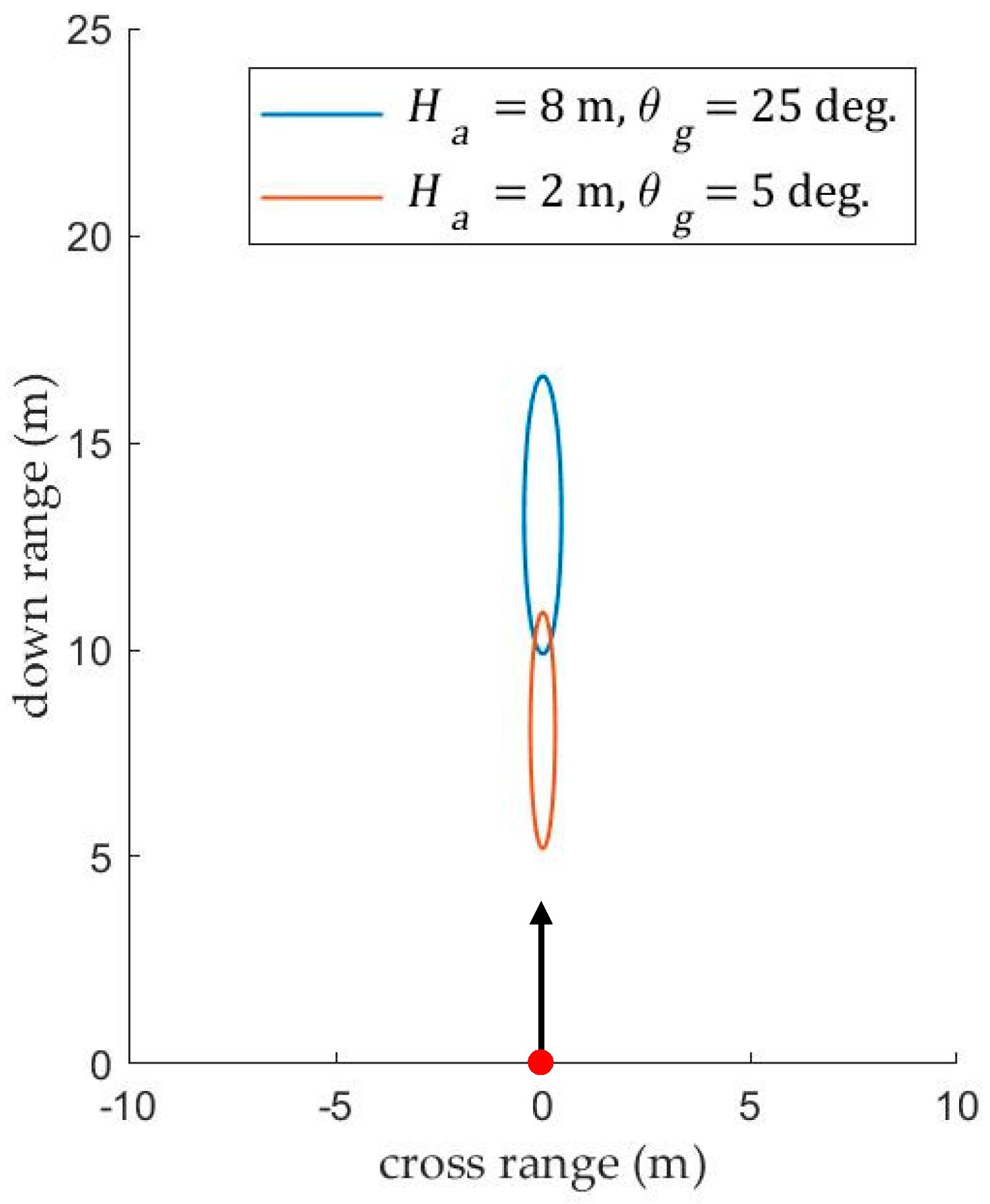
Two effective footprints. The radar is located at the red point (0, 0). The arrow points to the transmission direction. The sea surface is flat except for Bragg waves generated by an 8 m/s wind blowing towards the radar.
Figure 1.
Two effective footprints. The radar is located at the red point (0, 0). The arrow points to the transmission direction. The sea surface is flat except for Bragg waves generated by an 8 m/s wind blowing towards the radar.
Figure 2.
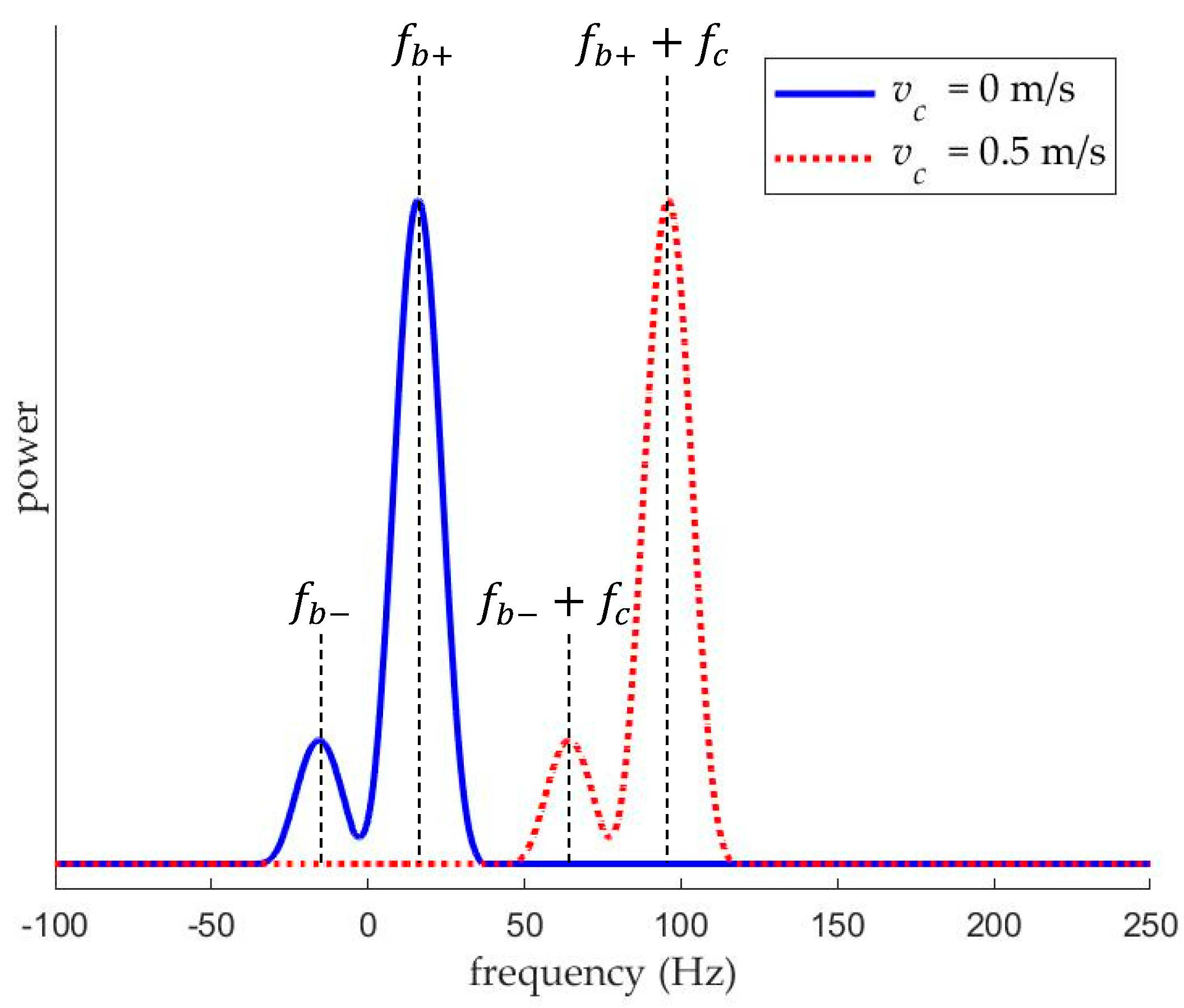
Two Bragg peaks in Doppler power spectrum. If = 0 m/s, two peaks present at −15.8 Hz and 15.8 Hz for receding and advancing Bragg waves, respectively, otherwise two peaks shift along the frequency axis. Here if = 0.5 m/s, two peaks shift right 80 Hz.
Figure 2.
Two Bragg peaks in Doppler power spectrum. If = 0 m/s, two peaks present at −15.8 Hz and 15.8 Hz for receding and advancing Bragg waves, respectively, otherwise two peaks shift along the frequency axis. Here if = 0.5 m/s, two peaks shift right 80 Hz.
Figure 3.
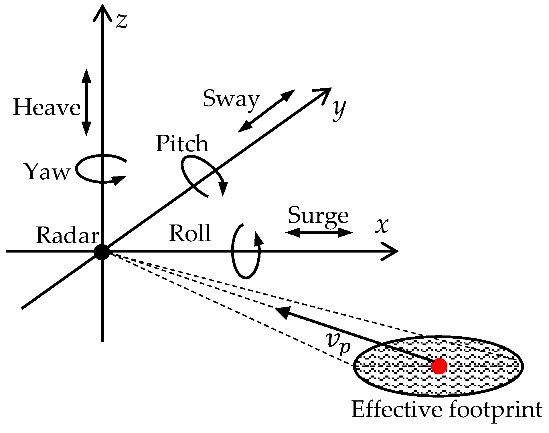
Three rotational motions and three linear motions of the K-band radar. The right-hand coordinate system xyz is built with the origin at the radar. The x-axis is parallel to the mean sea surface and follows the radar direction. Roll, pitch and yaw are rotational motions around x, y, and z-axes, respectively; surge, sway, and heave are linear motions along x, y, and z-axes, respectively. The center of the effective footprint is marked with the red point.
Figure 3.
Three rotational motions and three linear motions of the K-band radar. The right-hand coordinate system xyz is built with the origin at the radar. The x-axis is parallel to the mean sea surface and follows the radar direction. Roll, pitch and yaw are rotational motions around x, y, and z-axes, respectively; surge, sway, and heave are linear motions along x, y, and z-axes, respectively. The center of the effective footprint is marked with the red point.
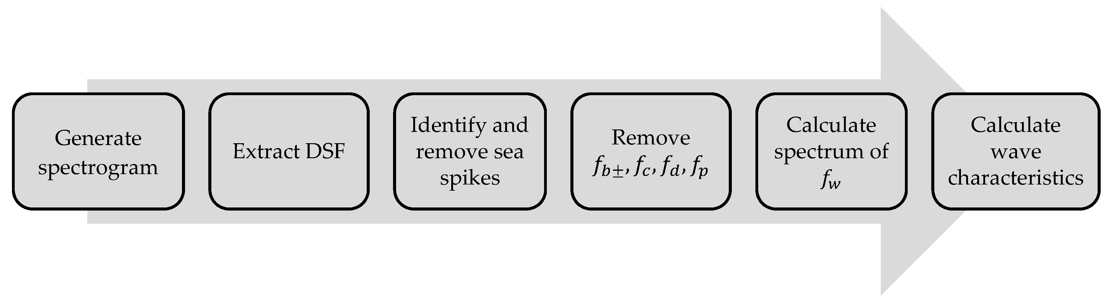
Figure 4.
Processing flow for the IF output of the K-band radar. DSF: Doppler shift frequency.
Figure 4.
Processing flow for the IF output of the K-band radar. DSF: Doppler shift frequency.
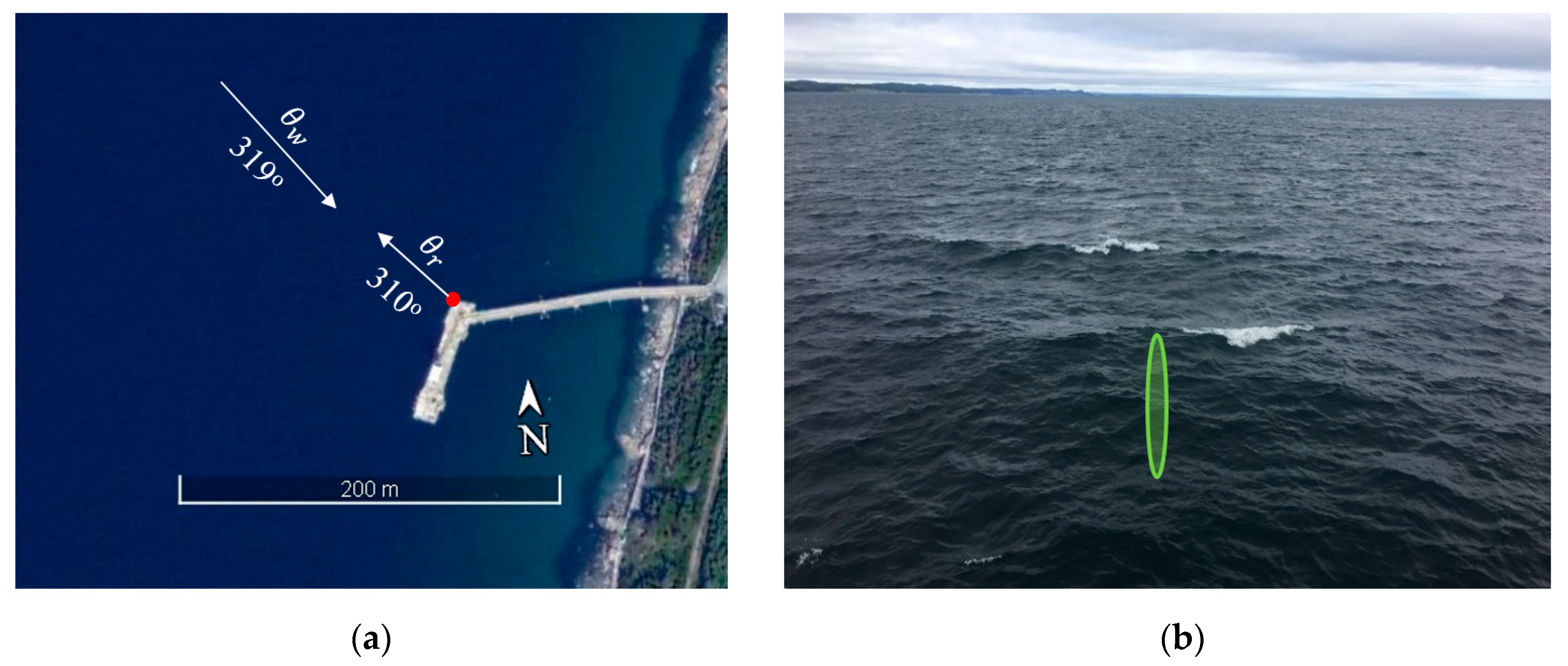
Figure 5.
(a) Bird view of the dock (from Google Maps). and are the wind direction and the radar looking direction, respectively. (b) Sea surface observed along the radar beam.
Figure 5.
(a) Bird view of the dock (from Google Maps). and are the wind direction and the radar looking direction, respectively. (b) Sea surface observed along the radar beam.
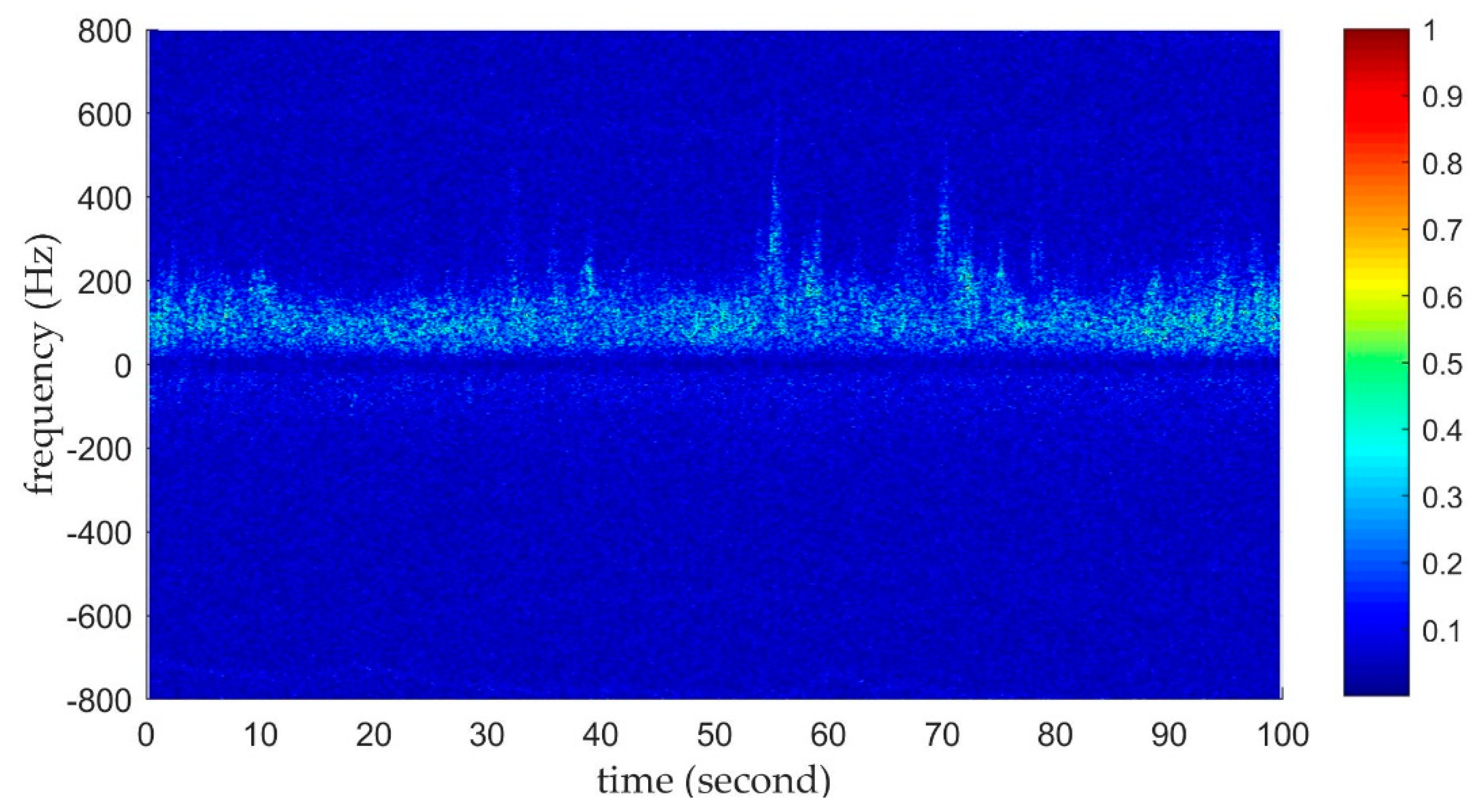
Figure 6.
Normalized power spectrogram of a 100-s IF output. The sampling rate is 1600 Hz. The resolutions of time and frequency are 0.1 s and 2 Hz, respectively.
Figure 6.
Normalized power spectrogram of a 100-s IF output. The sampling rate is 1600 Hz. The resolutions of time and frequency are 0.1 s and 2 Hz, respectively.
Figure 7.
DSF extraction and sea spikes identification. 75.8 Hz equates to twice the standard deviation of the extracted DSF.
Figure 7.
DSF extraction and sea spikes identification. 75.8 Hz equates to twice the standard deviation of the extracted DSF.
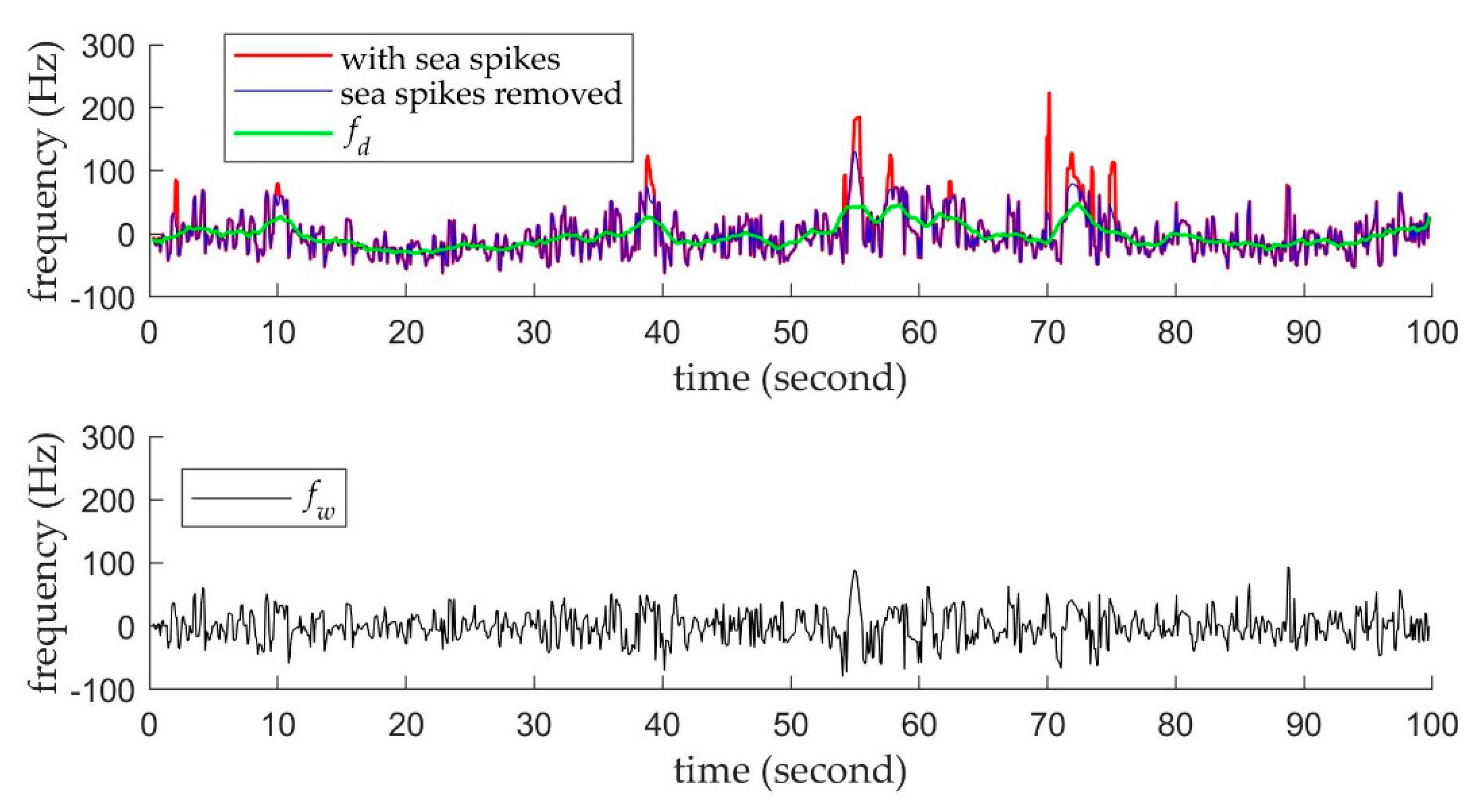
Figure 8.
Sea spike removal using moving average and the removal of .
Figure 8.
Sea spike removal using moving average and the removal of .
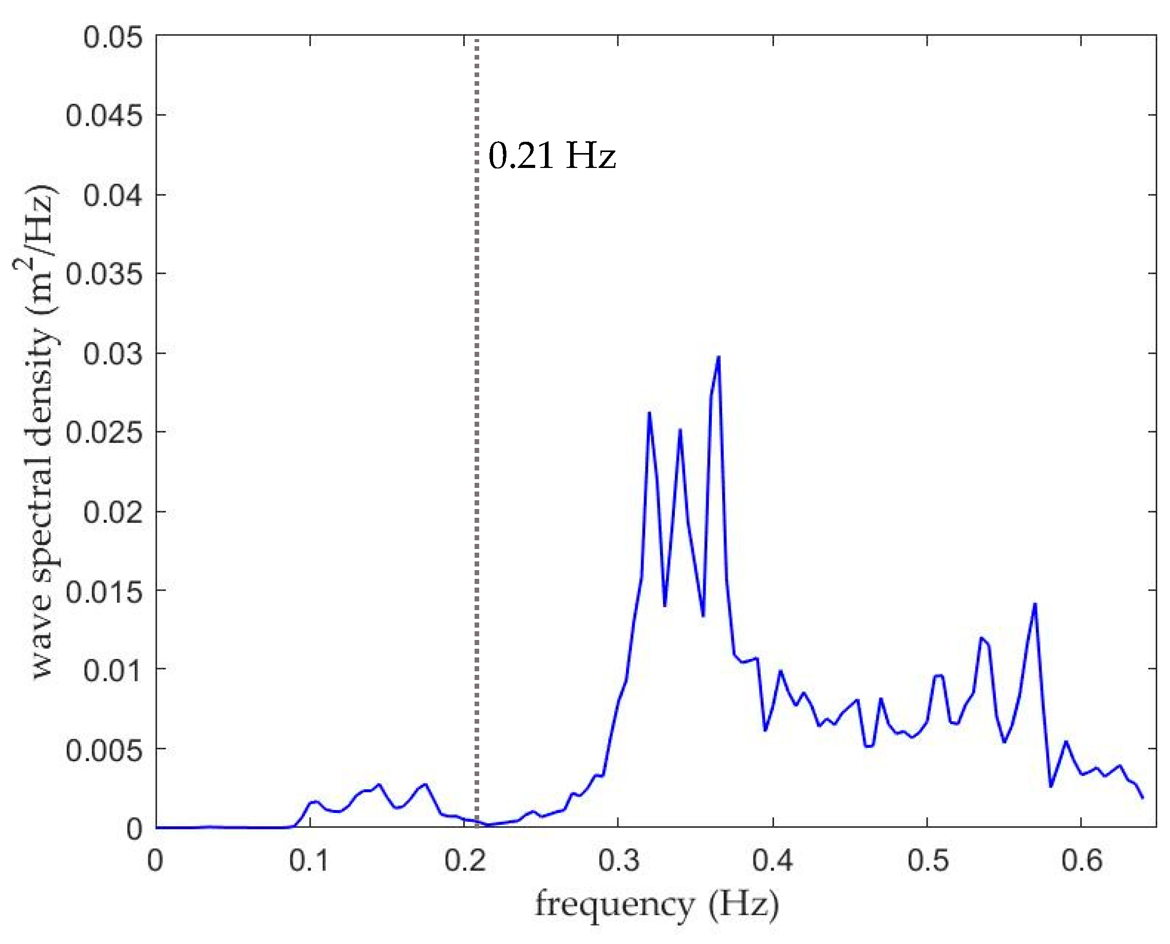
Figure 9.
The wave spectrum measured with a TRIAXYS Wave Buoy. It was located at (Latitude: 47°27.708′ N, Longitude: 53°6.498′ W) and operated by Marine Institute of Memorial University of Newfoundland. More information is available at SmartAtlantic.ca.
Figure 9.
The wave spectrum measured with a TRIAXYS Wave Buoy. It was located at (Latitude: 47°27.708′ N, Longitude: 53°6.498′ W) and operated by Marine Institute of Memorial University of Newfoundland. More information is available at SmartAtlantic.ca.
Figure 10.
Amplitude spectrum of .
Figure 10.
Amplitude spectrum of .
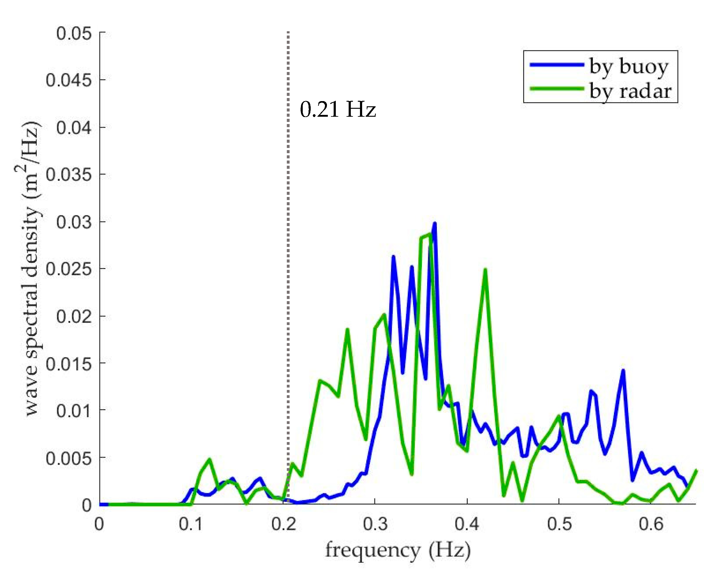
Figure 11.
Wind wave spectra measured by buoy and radar.
Figure 11.
Wind wave spectra measured by buoy and radar.
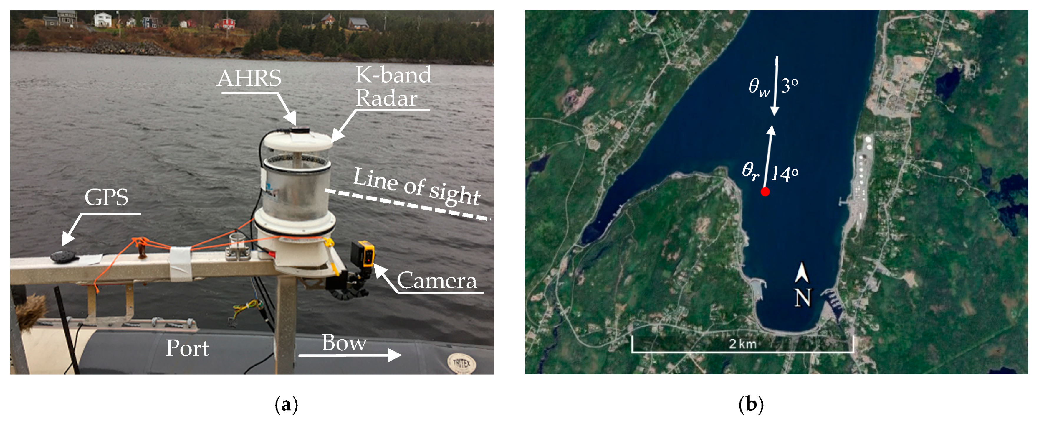
Figure 12.
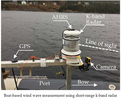
(a) Radar and auxiliary sensors on the boat. (b) Location of the experiment.
Figure 12.
(a) Radar and auxiliary sensors on the boat. (b) Location of the experiment.
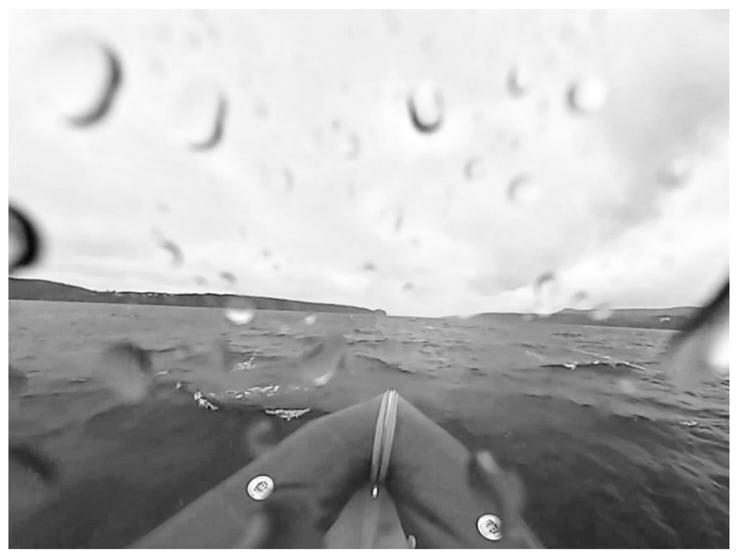
Figure 13.
Sea surface observed at the bow of the boat. Some raindrops partially obscured the camera lens.
Figure 13.
Sea surface observed at the bow of the boat. Some raindrops partially obscured the camera lens.
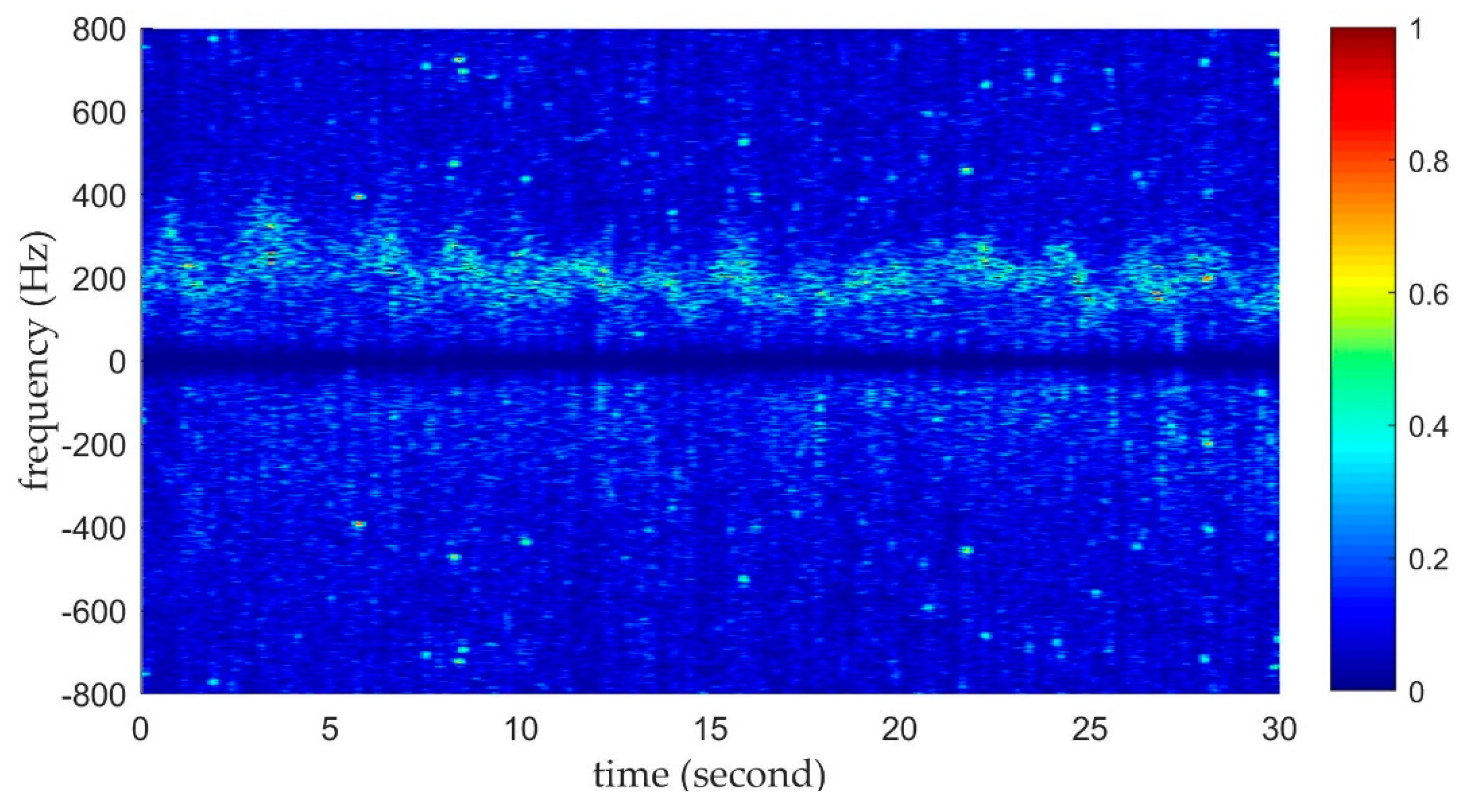
Figure 14.
Normalized power spectrogram of a 30-s IF output of the K-band radar. The sampling rate is 1600 Hz. The resolutions of time and frequency are 0.1 s and 2 Hz, respectively.
Figure 14.
Normalized power spectrogram of a 30-s IF output of the K-band radar. The sampling rate is 1600 Hz. The resolutions of time and frequency are 0.1 s and 2 Hz, respectively.
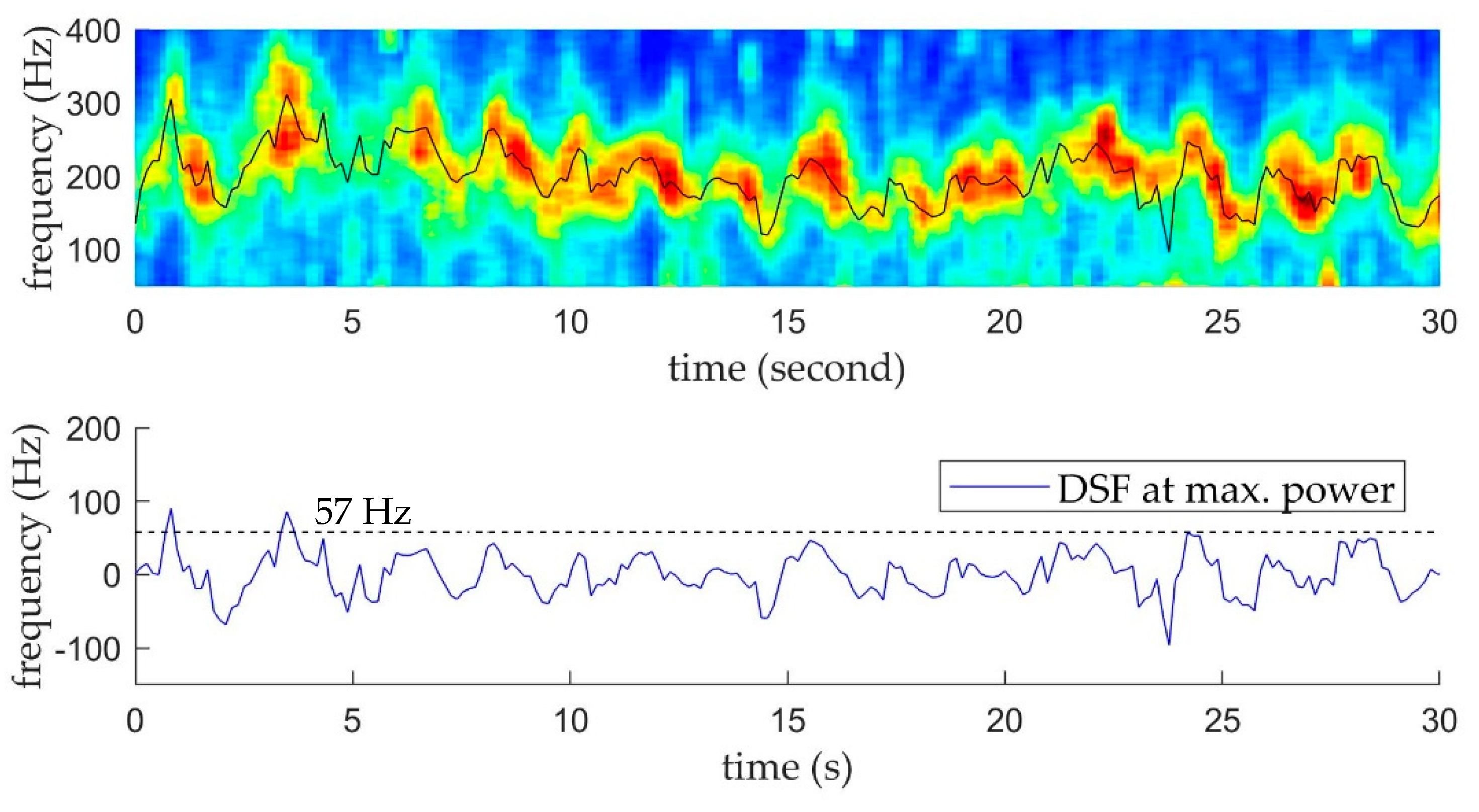
Figure 15.
DSF extraction from the processed spectrogram and sea spikes identification.
Figure 15.
DSF extraction from the processed spectrogram and sea spikes identification.
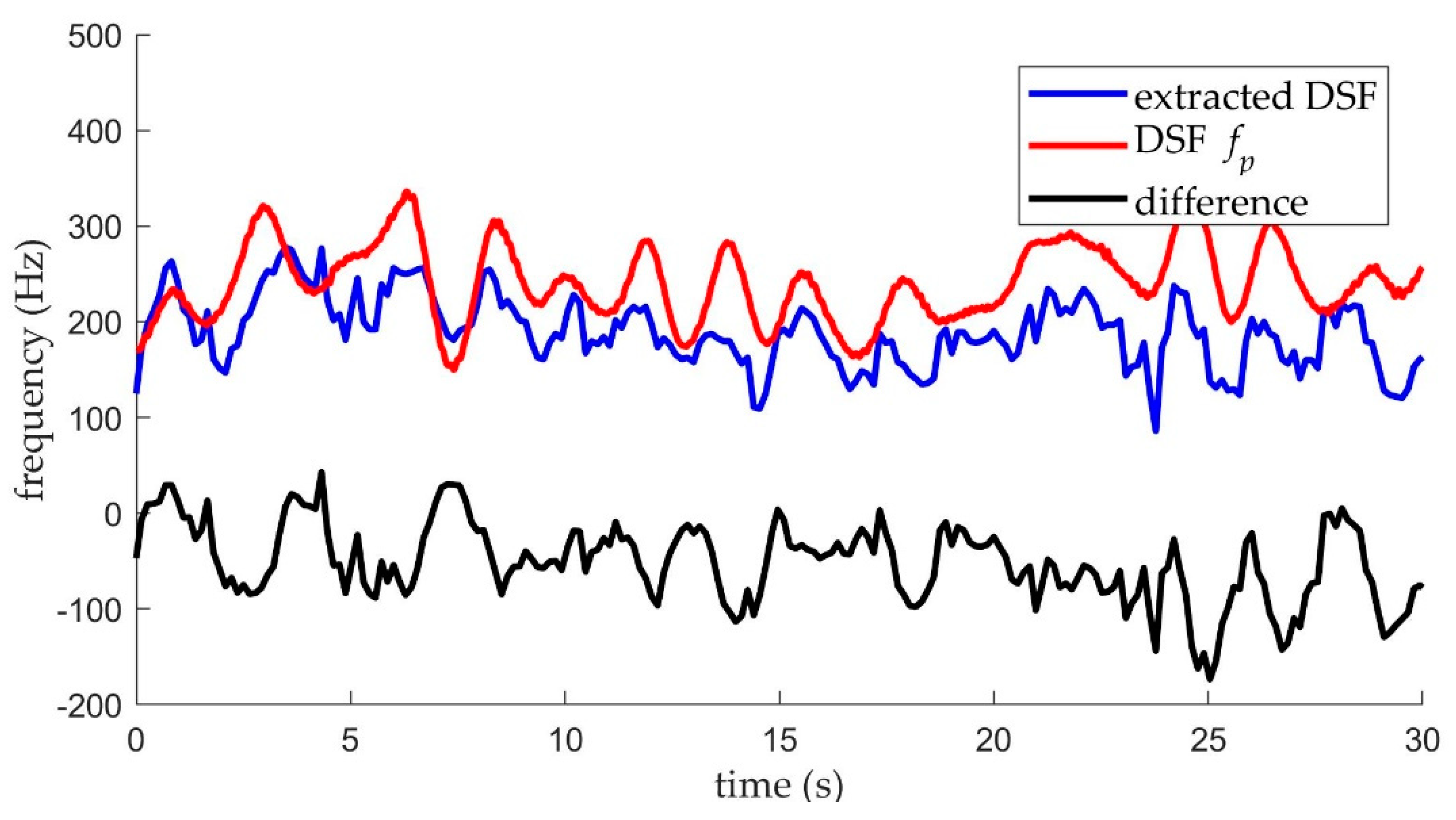
Figure 16.
Removal of DSF .
Figure 16.
Removal of DSF .
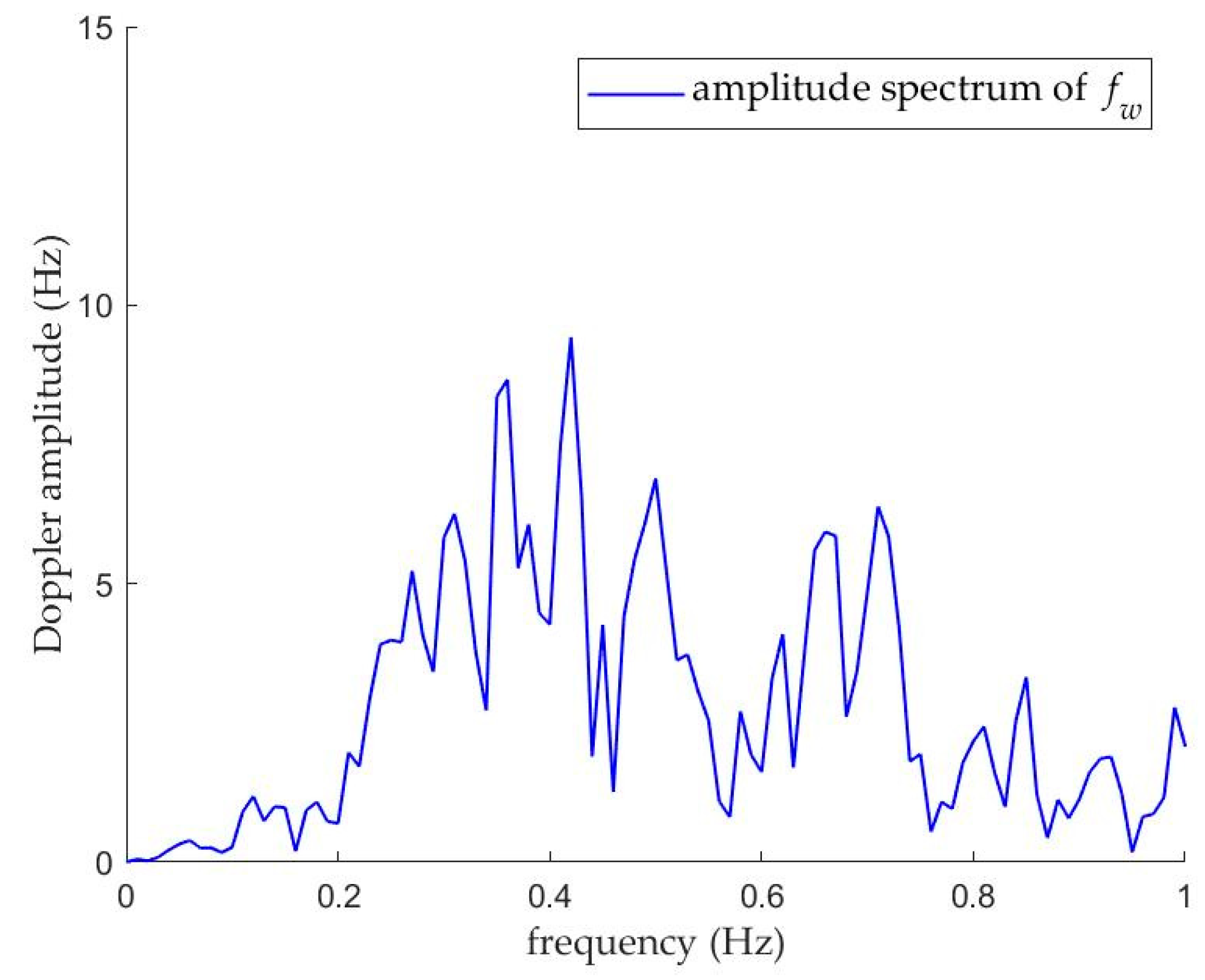
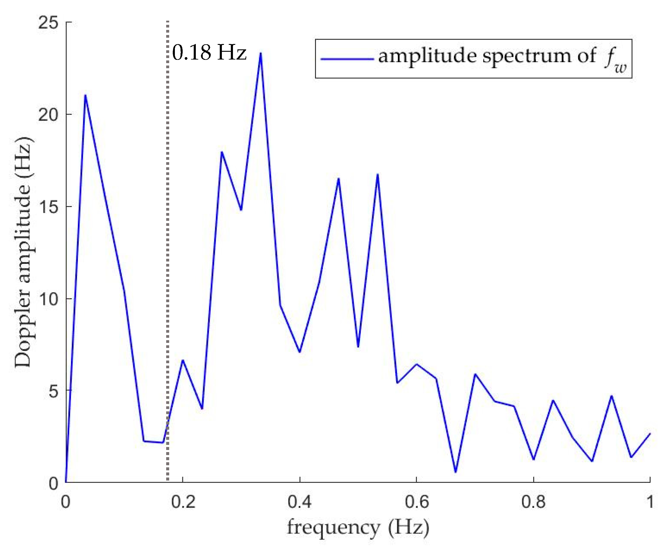
Figure 17.
Amplitude spectrum of .
Figure 17.
Amplitude spectrum of .
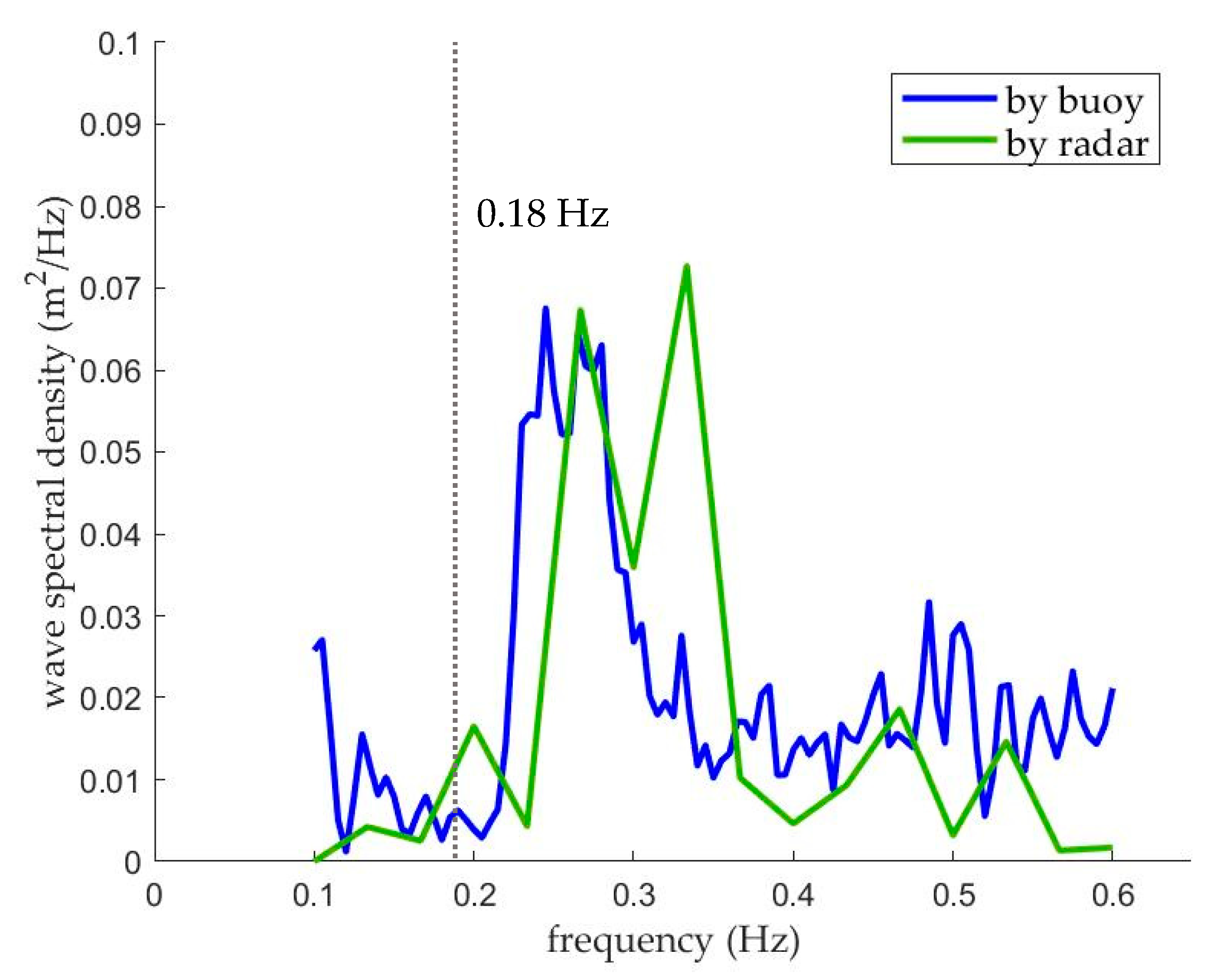
Figure 18.
Wind wave spectra measured by buoy and radar.
Figure 18.
Wind wave spectra measured by buoy and radar.
Table 1.
Conditions of radar antenna and wind.
Table 1.
Conditions of radar antenna and wind.
| | Parameters | Notation | Value | Unit |
|---|
| Radar antenna | Transmission frequency | | 24 | GHz |
| Horizontal -3dB beam width | - | 7 | degree |
| Vertical -3dB beam width | - | 25 | degree |
| Wind | Wind speed | | 8 | m/s |
| Wind direction | - | 0 (upwind) | degree |
Table 2.
Two calculation examples of and .
Table 2.
Two calculation examples of and .
| a (meter) | T (second) | L (meter) | | | | |
|---|
| 0.20 | 2 | 6.2 | 3.14 | 1.01 | 0.13 | 20.3 |
| 0.30 | 3 | 14.0 | 2.09 | 0.45 | 0.08 | 13.5 |
Table 3.
Settings of radar and conditions of wind and wave.
Table 3.
Settings of radar and conditions of wind and wave.
| Parameters | Notation | Value | Unit |
|---|
| Radar | Height from sea level | | 7.3 | meter |
| Direction to | | 310 | degree |
| Grazing angle | | 25 | degree |
| Transmission frequency | | 24 | GHz |
| Wind | Direction from | | 319 | degree |
| Average speed | | 7.3 | m/s |
| Wave | Significant wave height | | 0.24 | meter |
| Mean wave period | | 2.4 | second |
Table 4.
Characteristics of wind waves.
Table 4.
Characteristics of wind waves.
| Device | | |
|---|
| Buoy | 0.24 | 2.4 |
| Radar | 0.25 | 1.9 |
Table 5.
Settings of radar and conditions of wind, wave, and boat.
Table 5.
Settings of radar and conditions of wind, wave, and boat.
| Parameters | Notation | Value | Unit |
|---|
| Radar | Height from sea level | | 2 | meter |
| Direction to | | 14 | degree |
| Grazing angle | | 5 | degree |
| Transmission frequency | | 24 | GHz |
| Wind | Direction from | | 3 | degree |
| Average speed | | 8.4 | m/s |
| Wave | Significant wave height | | 0.41 | meter |
| Mean wave period | | 2.7 | second |
| Boat | Ground speed | | 0.53 | m/s |
Table 6.
Characteristics of wind waves.
Table 6.
Characteristics of wind waves.
| Device | | |
|---|
| Buoy | 0.41 | 2.7 |
| Radar | 0.38 | 2.9 |


